6.1 How Taxes and Subsidies Change Market Outcomes
I bet that you drink sugar-laden drinks at least now and again. Most Americans do, and roughly one in three do so every day. So if you have a daily soda habit, you aren’t alone. But chances are that you also think you should try to cut back. Soda is a big source of sugar in our diets and it isn’t good for us. It’s not just that it’ll rot your teeth, it can also lead to heart disease, diabetes, and high blood pressure.

Sweet and bubbly and subject to government intervention.
Sugary drinks are the biggest source of added sugar in most people’s diets. As a result, the World Health Organization has implored governments to help cut soda consumption. That’s why many countries and many cities in the United States have introduced special taxes on sugar-sweetened beverages. The idea behind these “soda taxes” is to drive up the price of sugary drinks so people will drink fewer of them.
These policies have sparked lots of debate about the government’s role in both driving up prices of soda for consumers and driving down sales and prices received by soda sellers. That’s in fact exactly what taxes typically do—they tend to reduce the quantity demanded and the quantity supplied of the taxed good as buyers pay more and sellers receive less. Why the difference between the price buyers pay and the price sellers receive? Because the government takes a cut in the form of a tax.
You and your friends may disagree about whether this policy makes people better off. Some argue that people should have the right to buy as much soda as they want at market prices—in essence deciding for themselves how much to drink. Others argue that people are overconsuming soda because they aren’t fully taking into account the negative effects on their health later in life and on the health care system.
We’ll focus on evaluating these arguments in later chapters. For now, our goal is to understand how the tax changes the quantity sold and the prices buyers pay and sellers receive. Let’s see how all this works by analyzing a tax on sugary beverages that came into effect in Philadelphia in 2017.
A Tax on Sellers
In 2017, Philadelphia introduced a tax on sellers of sugar-sweetened beverages of 1.5 cents per ounce. The way the tax works is that when you buy a 20-ounce soda, you’ll pay whatever price the seller posts and you don’t have to worry about the tax. The seller keeps whatever you pay minus the new tax, because they’re responsible for sending the tax to the government. This is a tax on sellers because, if you buy a 20-ounce soda, the seller needs to send $0.30 ($0.015 per ounce × 20 ounces) to the government.
A tax on sellers shifts the supply curve.
The tax represents a marginal cost to sellers because it’s an additional cost they must pay for each unit they sell. You learned in Chapter 3 that the supply curve is the marginal cost curve. Therefore, when marginal costs increase, the supply curve shifts. This is the interdependence principle in action, illustrating how the choices of others—in this case, the government—affect your decisions.
Figure 1 shows the market for soda in Philadelphia. Before the tax is implemented, the supply curve intersects the demand curve at 1.4 million bottles of 20-ounce sodas sold per week, at an equilibrium price of $1.10 per bottle. Philadelphia’s soda tax adds $0.30 to the marginal cost of a 20-ounce bottle of soda, causing supply to decrease. Typically, we describe a decrease in supply as shifting the supply curve to the left. In this case, you might find it easier to think about the supply curve shifting up by the amount of the increase in marginal costs. Since the supply curve is the marginal cost curve, if marginal costs are $0.30 higher, then the supply curve must shift $0.30 up.
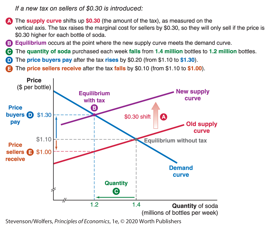
Figure 1 | Effects of Taxing Soda Sellers in Philadelphia
The tax leads to a decline in the quantity sold.
The shift in supply results in the new supply curve intersecting the demand curve at a lower quantity demanded. The quantity of soda sold declines from 1.4 million bottles per week to 1.2 million bottles. The end result is that higher soda prices lead to lower soda sales because each bottle of soda costs consumers more.
The tax increases the price buyers pay and decreases the price sellers receive.
The new price of $1.30 is the price you pay at the register for a 20-ounce soda, but it isn’t the amount that sellers keep, since they have to send the government $0.30 per bottle in taxes. Thus, Figure 1 shows that at the new equilibrium, the price buyers pay for soda rises from $1.10 to $1.30, an increase of $0.20. But sellers, who have to send $0.30 per soda to the government, only keep $1.00 ($1.30 minus $0.30), a fall of $0.10 from the equilibrium price without taxes of $1.10.
Both buyers and sellers bear the economic burden of the tax on sellers.
There is an important distinction between who is assigned by the government to send a tax payment and who ultimately bears its burden. The statutory burden of a tax describes the burden of being assigned by the government the responsibility of sending a tax payment. But if you want to know who experiences a greater loss as a result of the tax, you should focus instead on the economic burden, which describes the burden created by the change in after-tax prices faced by buyers and sellers as a result of the tax.
In Philadelphia, the statutory burden is entirely a tax on sellers—after all, they are responsible for sending in the full payment to the government. However, buyers and sellers each bear some of the economic burden. Even though the tax is $0.30, the price sellers get to keep after they send in the tax payment is only $0.10 less than the pre-tax equilibrium price of $1.10. Buyers of soda—like you—make up the difference because you pay $0.20 more per soda than you would without the tax.
Effectively then, buyers and sellers are sharing the economic burden of the soda tax. In our example, buyers bear a larger share of the economic burden of a soda tax. Economists have estimated the economic burden of soda taxes and have found that about two-thirds of a tax on soda tends to fall on consumers. Tax incidence describes the division of the economic burden of a tax between buyers and sellers.
A Tax on Buyers
Instead of taxing soda sellers, the government could change the statutory burden and levy a tax on soda buyers. Practically, the way this typically works is that stores post the price without the tax, you pay the tax as you check out, and the store does you the convenience of mailing in the tax. But it’s just that, a convenience. You may not realize it, but when the government levies a tax on buyers, the buyer is responsible for submitting the payment to the government if the store doesn’t do it for them. So, when you thought you were getting a deal buying stuff online from websites that don’t collect your local sales tax, technically you were supposed to figure out the sales tax and include the payment with your annual tax return.
So what happens if we switch the statutory burden to buyers? The price posted at store is the before-tax price and reflects what the store receives without the tax. Buyers, however, have to pay that price plus the $0.30 per soda tax when they get to the register. You might be used to this, since you’ve probably paid a sales tax before that works this way.
A tax on buyers shifts the demand curve.
In Chapter 2, you learned that the demand curve is the marginal benefit curve. A tax of $0.30 reduces the marginal benefit of buying a soda by $0.30, because that soda now comes with a 30-cent tax obligation. As such, a tax on buyers causes a decrease in demand. This is the interdependence principle in action, showing how the choices of others—in this case, the government—affect your decisions. Typically, we describe a decrease in demand as shifting the demand curve to the left. But when you’re analyzing a tax, you might find it easier to think about the demand curve shifting down by the amount of the tax. The reason that the demand curve in Figure 2 shifts down by $0.30 is that buyers will only be willing to purchase the same quantity as before only if the pre-tax price is $0.30 lower.
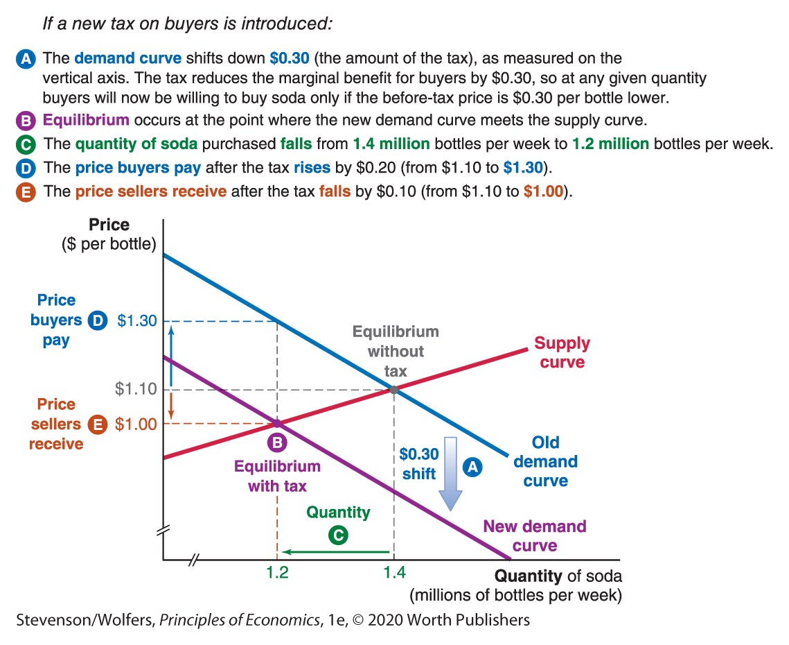
Figure 2 | Effects of Taxing Soda Buyers in Philadelphia
The tax leads to a decline in the quantity sold.
Following the shift in demand, the new demand curve intersects the supply curve at a lower quantity supplied. The quantity of soda sold declines from 1.4 million bottles per week to 1.2 million and the price that sellers charge for each bottle declines from $1.10 to $1.00. But the price buyers pay is both the price the store charges and the tax payment they must make. So buyers now pay $1.30 (the new store price of $1.00 plus an additional $0.30 tax), which is $0.20 cents per soda more than the $1.10 they paid before the tax.
The tax increases the price buyers pay and decreases the price sellers receive.
Let’s unpack what’s happening with the price a bit more. Figure 2 shows that the sellers’ price declines from $1.10 to $1.00 per soda. Thus, the price received by sellers has fallen by $0.10 per soda. Meanwhile, the price buyers pay has risen, from $1.10 per soda to $1.30 (that is, $1.00 per soda plus the $0.30 tax), and so the after-tax cost of a 20-ounce soda has risen by $0.20.
Buyers and sellers bear the economic burden of a tax on buyers.
The statutory burden is simple: This is a tax levied on buyers. But what about the economic burden? We’ve found that a tax on buyers of $0.30 per soda raises the price buyers pay for soda (including taxes) by $0.20 per soda. In turn, the price sellers receive has declined by $0.10 per soda, from $1.10 to $1.00. Thus, buyers and sellers share the economic burden of this tax.
The Statutory Burden and Tax Incidence
It doesn’t matter whether it is the buyer or the seller who puts the money into the tax jar.
We’ve just uncovered a startling result: Whether the new soda tax is levied on buyers or sellers, it has the same economic effect! Go back and compare the previous two examples. Taxing sellers $0.30 per soda (as in Figure 1) led the equilibrium quantity of soda to decline from 1.4 million sodas per week to 1.2 million. The price paid by buyers rose from $1.10 to $1.30 per soda, while the price received by sellers (after they’ve paid their tax obligations) fell from $1.10 to $1.00. Placing the statutory burden on buyers instead (as in Figure 2) also led the equilibrium quantity of soda sold to decline from 1.4 million sodas per week to 1.2 million. And it also led the cost to the buyer (that is, the price paid inclusive of the tax obligation) to rise from $1.10 per soda to $1.30, while the price sellers received fell from $1.10 per soda to $1.00. The numbers are identical! That is, a soda tax has exactly the same effects, whether it is assigned to buyers or sellers! This isn’t a coincidence, it’s a general insight about all taxes, so let me reinforce this: It doesn’t matter whether the buyer or seller is assigned by the government to send in the tax; the end result is exactly the same.
The fact that it doesn’t matter whether you levy a tax on buyers or sellers is a surprising finding that holds for all taxes. And just to be clear, I’m not saying that taxes don’t matter. When the government levies a tax, buyers buy less, sellers sell less, and prices are higher for buyers and lower for sellers. What is irrelevant, however, is whether the tax is levied on buyers or sellers. The tax matters, but who has the statutory burden turns out not to matter at all!
It doesn’t matter who puts the money into the tax jar.
Here’s a simple metaphor that might help explain this surprising finding. You’ve just picked out an ice-cold Coke, and you walk to the counter inside a convenience store to pay. A “tax jar” is sitting on the counter. You pull $1.30 out of your pocket to pay for the Coke. If the seller is assigned the statutory burden, you hand the seller $1.30. The seller, being responsible for submitting the tax, puts $0.30 of this into the “tax jar” and the remaining $1 into their cash register. If instead you’re assigned the statutory burden as the buyer, then what changes? You still pull the same $1.30 out of your pocket. The only thing that changes is that this time, you’re the one who puts the $0.30 into the “tax jar,” and you hand the shopkeeper the remaining $1.00 to put into their cash register. In both cases, the same $1.30 comes out of the buyer’s pocket, the same $1.00 goes into the shopkeeper’s cash register, and the same $0.30 goes into the tax jar. That is, the transactions among buyer, seller, and government are inherently the same, irrespective of whether the tax is assigned to buyers or sellers.
This yields a surprising conclusion: Neither buyers nor sellers should care about who has the statutory burden, because a change in the statutory burden doesn’t affect the economic burden they each face.
EVERYDAY Economics
Who pays for your Social Security?
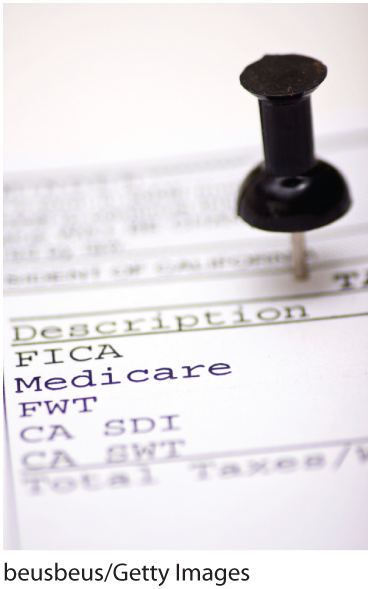
The deduction on your pay stub for the FICA (Federal Insurance Contributions Act) tax is your half of the payment toward your Social Security account.
The Social Security system in the United States is a federal government program that will provide you with retirement income. To fund this program, 12.4% of what you earn in wages is paid into Social Security. Either buyers of labor (your employer) or sellers of labor (you) could be asked to pay the tax, but instead, the statutory burden of Social Security is split evenly between employers and workers.
Each pay period, two payments are made to your Social Security account. The first payment comes from your employer, who sends an amount equal to 6.2% of your pay to Social Security. You don’t see this amount on your paycheck, but trust me, they pay it. The second payment is withheld from your paycheck, which typically lists 6.2% deduction for your Social Security contribution. Taxes to fund Medicare, the government-run health insurance program for seniors, function in a similar way: You pay a 1.45% tax on your paycheck, and your employer pays another 1.45%. So like Social Security, the statutory burden is borne half by your employer and half by you.
Many people think it sounds fair that you and your employer split the bill for these programs. But does splitting the statutory burden make a difference? How would things change if the law changed so employers no longer had to pay their half, and instead workers were assigned to foot the whole bill? Or what if employers paid the whole bill, and workers didn’t have to pay? Each of these alternatives would change the statutory burden of these taxes.
But as we’ve already established, the economic burden doesn’t depend on whether a tax is levied on the buyer of labor (your employer) or the seller (you). The outcome in terms of wages and workers employed won’t change. What would change would be the amount of pay you see on your paycheck (since right now you don’t see what your employer pays, but you do see what you are paying). Research shows that workers tend to bear most of the economic burden from Social Security taxes, because labor supply is fairly inelastic. That means that even if employers were asked to pay the entire 12.4%, people wouldn’t see much of a change in their take-home pay and employment wouldn’t change. So, while splitting the bill with your employer seems “fair,” it’s also politically motivated fiction. The same outcomes would occur even if you (or, alternatively, your employer) were required to pay for all your Social Security contributions.

The Economic Burden of Taxes
City officials in Philadelphia argued that a soda tax would raise needed revenue from the soda industry to fund education. But others argued that these taxes would hurt consumers since a soda tax will raise the price consumers pay for soda. These are arguments about tax incidence: Who is going to bear the economic burden of the tax—soda suppliers or soda buyers?
Tax incidence depends on the price elasticity of demand and supply.
Tax incidence depends on your ability to avoid taxes—the more that you can avoid the tax, the less of it you will pay (and thus the lower your economic burden). The way to avoid a tax is to not buy or sell things that are taxed. In Chapter 5, you learned that the price elasticity of demand tells you how responsive buyers are to price changes and the price elasticity of supply tells you how responsive sellers are to price changes. Since taxes cause prices to change, it makes sense that the price elasticities of demand and supply determine who is best able to avoid a tax. Let’s explore this separately for buyers and sellers.
Sellers bear a smaller share of the economic burden when supply is relatively elastic.
If you’re a seller, the only way to avoid a tax hike is to supply a smaller quantity. Importantly, sellers experience a tax hike as a reduction in the after-tax price they receive. Sellers avoid a tax by decreasing the quantity they supply as the after-tax price they receive falls. If you owned a soda company, what would you do if you were taxed? Remember that the key to the elasticity of supply is how flexible the seller is. Can you easily switch to making another, nonsugary drink? Or producing a different type of product? The more flexibility sellers have to use their resources to do something differently, the more elastic the price elasticity of supply.
Figure 3 shows two graphs, each starting from the same market equilibrium prior to the tax being introduced and each adding the same 30-cent tax on soda. The difference between the two graphs is that supply is relatively elastic on the left and is more inelastic on the right. For the same tax added to the market, the price sellers receive will fall by less when supply is relatively more elastic (as shown at left in Figure 3). In contrast, when supply is relatively more inelastic (as shown at right in Figure 3), sellers bear more of the economic burden of the tax and therefore see a larger decline in the after-tax price. The larger the price elasticity of supply, the more sellers avoid the economic burden of the tax. And so the more elastic a seller’s supply curve is, the smaller their share of the economic burden.

Figure 3 | Price Elasticity and Tax Incidence
Buyers bear a smaller share of the economic burden when demand is relatively elastic.
As a consumer, you can avoid a soda tax by buying fewer sodas. In fact, you won’t pay any soda tax if you don’t buy any soda. The more you reduce the quantity you demand in response to a tax-induced price hike, the more you are effectively avoiding the tax, leaving sellers to pay more. Your price elasticity of demand—that is, your responsiveness to an increase in price—is determined by the substitutes available to you. What would you do if the price of soda went up? Would you switch to a nonsugary beverage?
The left side of Figure 3 shows demand that is inelastic relative to supply. In this case, buyers are not very responsive to changes in price relative to sellers. As a result, a larger share of the economic burden falls on buyers. So if you are an advocate representing the interests of consumers, an important question to ask when analyzing the likely impact of a soda tax is how willing are consumers to give up soda?
The more consumers are willing to switch to unsweetened coffee, tea, water, and juices, the more elastic their demand curve is. And when demand is relatively elastic, as in the right side of Figure 3, their share of the tax incidence will be smaller. Recall that both figures show the same $0.30 tax being added to the market, but the price increase that buyers face differs substantially. The price increase buyers face is lower when demand is relatively more elastic.
Recap: The factor that is more elastic will have a smaller share of the economic burden.
In the end, the full amount of the tax will get sent to the government, and the question is where did the money really come from. When the price elasticity of demand is large relative to the price elasticity of supply, then buyers bear a smaller share of the economic burden. In this case, the money is coming from sellers who have to lower their prices by more to keep customers. By contrast, if the price elasticity of supply is larger, then the share of the economic burden paid by sellers is smaller. In this case, the money is coming from buyers who pay higher prices rather than giving up a lot of consumption. The end result is that whichever factor is more elastic bears less of the economic burden of the tax. The underlying logic is that you can “get out of the way” of taxes by changing the quantities you buy or sell. And whoever has the largest elasticity “gets out of the way” more effectively.
When it comes to soda, buyers’ demand is relatively more inelastic than sellers’ supply. Researchers have shown that buyers typically bear about two-thirds of the economic burden of the tax, while sellers bear a third. Why? It essentially comes down to tastes. People like sugary drinks and therefore don’t find other substitutes quite as good; sellers, on the other hand, have a bit more flexibility to sell other products.
A Three-Step Recipe for Evaluating Taxes
Let’s step back and see that to analyze these taxes we followed the same three-step recipe for predicting market outcomes that you used to find market equilibriums in Chapter 4. When you’re analyzing a new tax, ask these three questions:
- Step one: Is the supply or demand curve shifting? Remember that any change affecting buyers or their marginal benefits will shift the demand curve, while any change affecting sellers or their marginal costs will shift the supply curve. (Although given what you learned about the economic burden of a tax, it really doesn’t matter which curve shifts!)
- Step two: Is that shift an increase in taxes, shifting the curve to the left? Or is it a decrease in taxes, shifting the curve to the right? Taxes will typically shift the supply or the demand curve to the left because they are a cost that reduces the marginal benefit for consumers when they are assigned the statutory burden of a tax and raises the marginal cost for sellers when they are the ones who are assigned to send in the tax. A decrease in marginal benefit is a decrease in demand (a shift to the left or down). On the supply side, an increase in marginal cost causes a decrease in supply (a shift to the left or up).
- Step three: How will prices and quantities change in the new equilibrium? Compare the pre-tax equilibrium with the post-tax equilibrium. There is one complication to remember with taxes: There are really two prices—the price the buyer pays and the price the seller receives. Remember that these prices are after taxes. So you’ll need to be careful to distinguish which of these prices you’re thinking about.
Now you can practice following this recipe by working out what will happen with a tax on gas.
Do the Economics
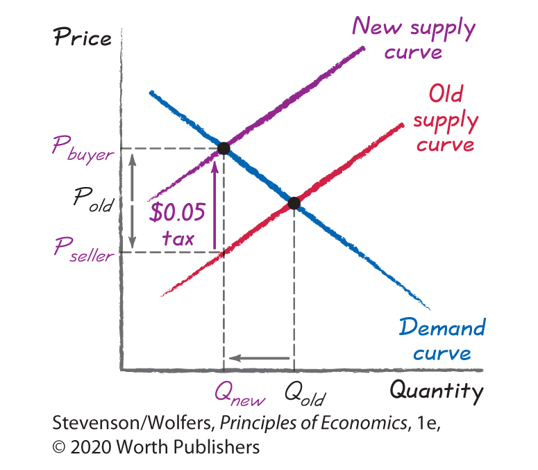
Michigan introduced a new tax of $0.05 per gallon of gas sold by gas stations in their state. Sellers will pay this tax directly to the government, meaning the tax will already be incorporated into the price you see when you drive by the gas station. How does this affect market outcomes?
Let’s work through the three-step recipe to find out.
- Step one: Is the supply or demand curve shifting?
The supply curve shifts because the tax is paid by sellers.
- Step two: Is that shift an increase in taxes, shifting the curve to the left? Or is it a decrease in taxes, shifting the curve to the right?
An extra tax on sellers will raise their marginal costs, since they have a new expense for each additional gallon sold: the money they need to send to the government. And higher marginal costs decrease supply, shifting the supply curve to the left (up). Because the tax is $0.05 per gallon, the supply curve shifts left (up) until it lies $0.05 higher as measured on the vertical axis.
- Step three: How will prices and quantities change in the new equilibrium?
The quantity of gas sold will decrease, the price sellers receive after the tax will fall, and the price buyers pay will increase.

Analyzing Subsidies
So far we’ve considered taxes, but what if instead of charging a tax, the government were to give a subsidy? A subsidy is a payment made by the government to those who make a specific choice. For example, a Pell Grant is a subsidy that the government gives lower-income people who choose to go to college. The government uses subsidies to try to encourage the consumption of certain goods and services, such as education.
It turns out that you can use the same three-step recipe you just learned to analyze a tax to understand how quantity demanded, quantity supplied, and price will change when the government offers a subsidy. One way to think about a subsidy is as a negative tax since it operates just like a tax, but with the opposite sign. Subsidies increase the quantities demanded and supplied, and they tend to lower the price buyers pay and increase the price sellers receive. And just like a tax, the outcomes don’t depend on the statutory assignment of the subsidy.
To see what happens with a subsidy, let’s consider a specific example. Governments around the world want to ensure that kids receive good early childhood education and that parents are able to work. As a result, they often subsidize child-care costs. The United States offers a range of subsidies to parents to help them manage the costs of child care, and policy makers have debated whether to increase these subsidies further.
Consider a proposal to pay parents of young children a $3,000 subsidy for child care. When the director of a child-care center asks you to predict the likely outcomes for the number of children seeking slots in the child-care market, you now know how to respond: Work through the three-step recipe we developed to analyze a tax change.
The first step is to ask: Is the demand or supply curve shifting? Since the subsidy will be given to parents who put their children in child care, the subsidy will shift the demand curve. At each price parents’ willingness to put their child in child care will be higher. This is because parents will receive care and a $3,000 payment from the government when they choose to put their kid in child care. So the marginal benefit of using child care has gone up. Notice that we are analyzing this is an “either/or” question—parents can either put their child in professional child care or keep them at home. Because many parents have to pay weekly or even monthly for a slot at a child-care center, this is a reasonable simplification.
The second step is to ask: Is this shift an increase in subsidies, shifting the curve to the right? Or is it a decrease in subsidies, shifting the curve to the left? A subsidy to consumers always increases demand by raising consumers’ marginal benefit by the amount of the subsidy. Parents will be more willing to purchase child care at any given price, because the “effective price”—after the subsidy—is lower. Another way to think about it is that they are willing to pay more because each child-care slot will come with a $3,000 check. So it adds $3,000 to the marginal benefit of putting a child in child care. So the demand curve shifts to the right or up by the amount of the subsidy as shown in Figure 4.
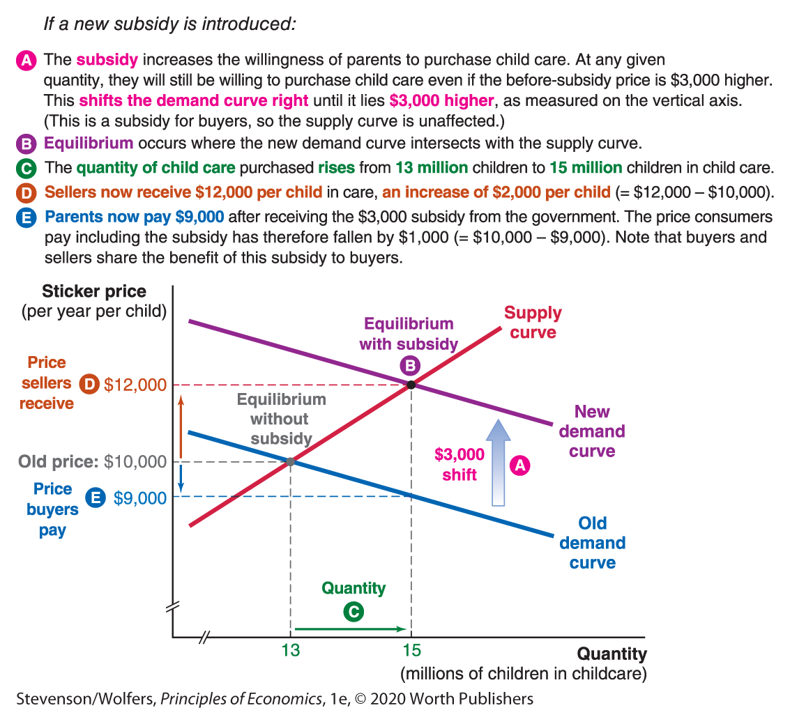
Figure 4 | Effects of Subsidizing Child Care
The third step is to ask: How will prices and quantities change in the new equilibrium? The demand curve shifts right and intersects the supply curve at a higher quantity supplied of child care. The result is a higher price for child-care providers. Prior to the subsidy parents paid $10,000 a year for child care. The after-subsidy demand curve intersects the supply curve at the higher price of $12,000 per year. As a result, child-care suppliers receive an increase of $2,000 per year. Parents pay $12,000 to the child-care suppliers, but receive a $3,000 payment. As such, the price parents pay after the subsidy falls from $10,000 per year to $9,000 per year.
Just as with the economic burden of taxes, the economic benefit of subsidies is shared between buyers and sellers. In this case, the price child-care providers receive goes up by $2,000, while the after-subsidy cost to parents falls by $1,000.
What determines the distribution of the subsidy between buyers and sellers? I bet you guessed it: the price elasticities of demand and supply. When demand is more elastic relative to supply, buyers capture less of a subsidy. Sellers capture more of the subsidy when their supply is inelastic. When supply is relatively more inelastic it means that a larger increase in price is needed to induce sellers to increase the quantity supplied to the level that buyers want. The opposite is true when demand is more inelastic relative to supply. If buyers have only a small change in their quantity demanded, then they will be able to capture more of the subsidy. In the extreme, when the price elasticity of demand is zero—meaning that a subsidy leads to no change in demand, then buyers will capture the entire subsidy. But if supply is completely inelastic, the opposite happens. In short, just like the elastic factor gets out of the way of taxes, the elastic factor gets out of the way of subsidies.
Just like with taxes, it doesn’t matter who gets the subsidy.
What if the government paid the subsidy to childcare providers instead so that each child-care provider received a payment from the government of $3,000 per child enrolled? Just like with taxes, the economic burden, or in this case we should say economic benefit, of subsidies is determined not by the statutory burden—who is assigned to get the subsidy, but by price elasticities of demand and supply. That means that we’d get the exact same outcome if the government sent the subsidy checks to child-care providers instead of sending them to parents. A subsidy sent to providers would shift the supply curve to the right or down by the amount of the subsidy and the outcome would be exactly the same: The new equilibrium quantity would be higher, buyers would pay less, and sellers would receive more in total, including the subsidy. Whether it’s a tax or a subsidy, it’s the laws of supply and demand not the laws set by government that determine who bears the economic burden of a tax and who gets the benefit of a subsidy.
Interpreting the DATA
How much of that Pell Grant do you really get?
Chances are you or someone you know has received a Pell Grant to help pay college tuition. The federal Pell Grant program provides billions of dollars in subsidies to low-income college students. But how much does this really help students who receive Pell Grants and how much does it benefit the schools they attend? You’ve seen that tax incidence (and subsidy incidence) depends on the price elasticity of demand and the price elasticity of supply. With a subsidy, the quantity typically increases and the price that suppliers receive goes up (while the price buyers pay goes down). But will schools really raise prices and take more students as a result of Pell Grants? The answer is yes to both questions. As a result of Pell Grants, more students are able to attend school and they pay less than they would without them. But students don’t capture 100% of the benefits. Researchers estimate that 12% of Pell Grant aid goes to schools because schools reduce the amount of aid they would give to low-income students. In effect, schools raise the price on low-income students a bit as a result of Pell Grants, by reducing the discounts they offer such students.
Now that we’ve dealt with how taxes shape economic behavior, let’s move on to another way in which governments try to reshape market outcomes: regulating prices directly.