14.2 Setting Prices When You Have Market Power
Figuring out what price to charge is one of the most important business decisions you’ll make. It’s a difficult balancing act. If you set your price too low, your profit margin will disappear. But if you set your price too high, then you’ll barely sell anything. You face a trade-off between selling a larger quantity of items versus making more money on each item you sell.
Figuring out how best to evaluate this trade-off is going to be a lot easier once we’ve introduced two new analytic tools—your firm’s demand curve, which summarizes your market power, and the marginal revenue curve, which measures your incentive to increase production. Let’s master these tools now, and then in a few pages’ time, we’ll use them to uncover an intuitive approach to pricing.
Your Firm Demand Curve
Your firm’s demand curve summarizes how the quantity that buyers demand from your individual firm varies as you change your price. Notice that your firm’s demand curve focuses on the quantity demanded from your specific firm. In contrast, the market demand curve describes the quantity demanded across all firms in the entire market. (It’s also different from an individual demand curve which describes the quantity demanded by a single buyer.)
Your market power determines the shape of your firm’s demand curve.
Consider first the extreme in which you have no market power, as in perfect competition. This situation is shown in the far left of Figure 2. With no market power, raising your price by even a penny will lead you to lose all your customers. Likewise, if you lower your price by just a penny, your competitors will lose all their customers to you, boosting your sales enormously. As a result, your firm’s demand curve is essentially flat because when there are many competitors selling the same product—perfect competition—a minuscule change in price leads to a nearly infinite change in the quantity you sell.

Figure 2 | Your Firm’s Demand Curve Depends on the Type of Competition You Face
The far right of Figure 2 shows the other extreme. If you are a monopoly—the only seller serving the market—then the quantity demanded from your firm is the same as the total quantity demanded by the entire market. As a result, a monopolist’s firm demand curve is also the market demand curve. Even though you have no competitors, a higher price will still lower the quantity demanded, because your customers still have the option of not buying your product.
Taken together, Figure 2 summarizes the close link between market structure, market power, and the price elasticity of demand along your firm’s demand curve. The two extremes bracket the more realistic case of imperfect competition, where you have some market power. Unlike perfect competition, you can raise your price without losing all of your customers. And unlike a monopolist, you face some competitors, and so raising your price will lead you to lose market share. Your firm’s demand curve can be relatively flat, or steep, depending on how much market power you have. If you don’t have much market power, then raising your price will sharply reduce the quantity you sell, and so your firm’s demand curve is relatively flat. (Alternatively phrased, it’s highly elastic.) By contrast, if you have a lot of market power, a price hike will lead you to lose very few sales, and so your firm’s demand curve is relatively steep (which is the same as saying it’s quite inelastic).
Experiment with your price to discover your firm’s demand curve.
Okay, how would you figure out how much market power you have and hence the shape of your firm’s demand curve? Here’s how businesses actually do it in practice: They experiment with the price they charge, and see how the quantity demanded varies in response. Indeed, a survey of large U.S. retailers revealed that 90% of them conduct pricing experiments.
Sometimes managers experiment with offering different prices to different groups of customers. For instance, when Amazon wanted to figure out its demand curve for popular movies, it programmed its website to show different prices to different customers. By comparing the quantity demanded by customers shown high prices with the quantity demanded by those shown low prices, they could map out their firm demand curve. (The customers who later learned they were offered a higher price were furious.)
Alternatively, some retailers experiment by charging different prices at different locations. For instance, the educational toy retailer Zany Brainy experimented with the price of a kids’ toy called the “Leapfrog Phonics Traveler,” charging $24.99 at some stores, $29.99 at a group of similar stores, and $34.99 in a third set of stores. The first group of stores sold 33 units, the second group sold 26, and the third group sold 15. Figure 3 shows the estimated firm demand curve, plotting the quantity demanded at each price (and then joining the dots).
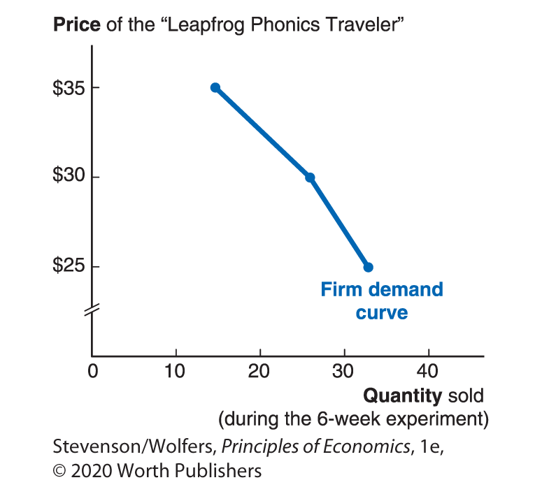
Figure 3 | Estimating Zany Brainy’s Firm Demand Curve
If you don’t have different locations, you can experiment by charging different prices over time, assessing how much higher the quantity demanded is when the price is lower.
Experimenting with the price you charge—whether it’s to different customers, in different locations, or at different times—can reveal your firm’s demand curve. And even though these experiments can be expensive, they’re often worth doing, because charging the wrong price can be even more expensive!
Do the Economics
Sofia runs a Ford dealership in Nashville, Tennessee. When she advertised the new Ford Focus at $23,000, she sold two cars per week. She then experimented with a discount, cutting the price to $22,000, which led her to sell three cars per week. A further price cut to $21,000 led sales to rise to four cars. And the week she experimented with a price increase, hiking the price to $24,000, she sold only one car.
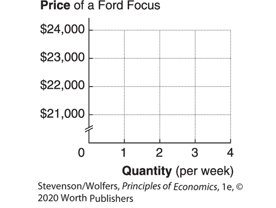
Plot the results of Sofia’s pricing experiments in the graph at right to discover her business’s demand curve.

Your Marginal Revenue Curve
Your firm demand curve is a critical input to making smart pricing choices, because it describes the trade-off between selling a larger quantity at a low price versus selling a smaller quantity at a higher price. Let’s explore how to use your firm’s demand curve to trace out how these alternatives affect your revenue.
Good decisions focus on marginal revenue.
Sofia wants to use the data she compiled in her pricing experiment to figure out what quantity of cars she should aim to sell, at what price.
Before proceeding, a reminder: The marginal principle tells you to break big decisions into smaller marginal decisions. So instead of asking how many cars she should sell, Sofia should ask whether she should sell one more car. To answer this, she needs to figure out her marginal revenue—the addition to total revenue she gets from selling one more car.
Calculate marginal revenue as the change in total revenue from selling one more unit.
You can use the data Sofia collected on her firm’s demand curve to calculate and plot her marginal revenue. To do this, she follows three steps. First, calculate total revenue, which is simply the price you charge times the quantity you sell. Second, assess her marginal revenue, which is the change in her total revenue from selling an additional car. Third, plot the results and you’ll get the marginal revenue curve, shown in Figure 4.

Figure 4 | Discover Your Firm’s Marginal Revenue Curve
Marginal revenue reflects the output effect, minus the discount effect.
Look closely at the table and the graph in Figure 4, and you’ll see we’ve just discovered something important: The marginal revenue Sofia gets from selling one more car is less than the price shown on the demand curve. This is true for all imperfectly competitive businesses. To see why, realize that there are two opposing forces affecting marginal revenue:
- The output effect: If Sofia sells one more car, her revenue will rise by the price she gets for it. This is the output effect: An extra unit of output will boost her revenue by an amount equal to the price of the extra item sold, P.
- The discount effect: To sell that one extra car, Sofia will have to lower her price a bit, which cuts into her revenue. Because this lower price applies to all of the cars she sells, even a small price cut might lead to a pretty big decline in revenue. This is the discount effect, and it’s equal to the price cut—that is, the discount she needs to give to sell one more car (call it ΔP, where the triangle symbol means “change”)—multiplied by the quantity she sells: ΔP × Q. (If this feels new to you, it is. Under perfect competition you can sell whatever quantity you want without needing to change your price, and so the discount effect is zero.)
Recall we began this section by noting that: You face a trade-off between selling a larger quantity of items versus making more money on each item you sell. Your marginal revenue curve neatly summarizes the terms of this trade-off. It tells you how much you’ll gain from selling a larger quantity of items (we call this part the output effect), less the revenue you’ll lose when you cut your price a bit, so you’re not making as much money on each item you sell (this bit’s the discount effect). Marginal revenue is the output effect, less the discount effect, and so it reflects the balance of these forces.
Marginal revenue lies below the demand curve, and it declines faster.
Let’s put together what we’ve learned about firm demand curves and marginal revenue.
- If you have market power, you can raise your price without losing all of your customers. This means your firm’s demand curve is downward-sloping.
- Due to the discount effect—that is, the need to cut your price a bit to sell that extra item—your marginal revenue from selling one more item is less than the price you charge for it. This means that your marginal revenue curve lies below your firm’s demand curve by an amount equal to the discount effect.
- The discount effect is bigger when you sell a larger quantity, because a price cut for many customers reduces revenue more than a price cut for just a few customers. As a result, the gap between your firm’s demand curve and marginal revenue widens as the quantity you sell increases. That’s why your marginal revenue curve declines more sharply than your firm’s demand curve.
Figure 5 also illustrates a helpful graphing trick: When the demand curve is a straight line, the marginal revenue curve is also a straight line that starts at the same point (when the quantity is one), but it declines twice as sharply.
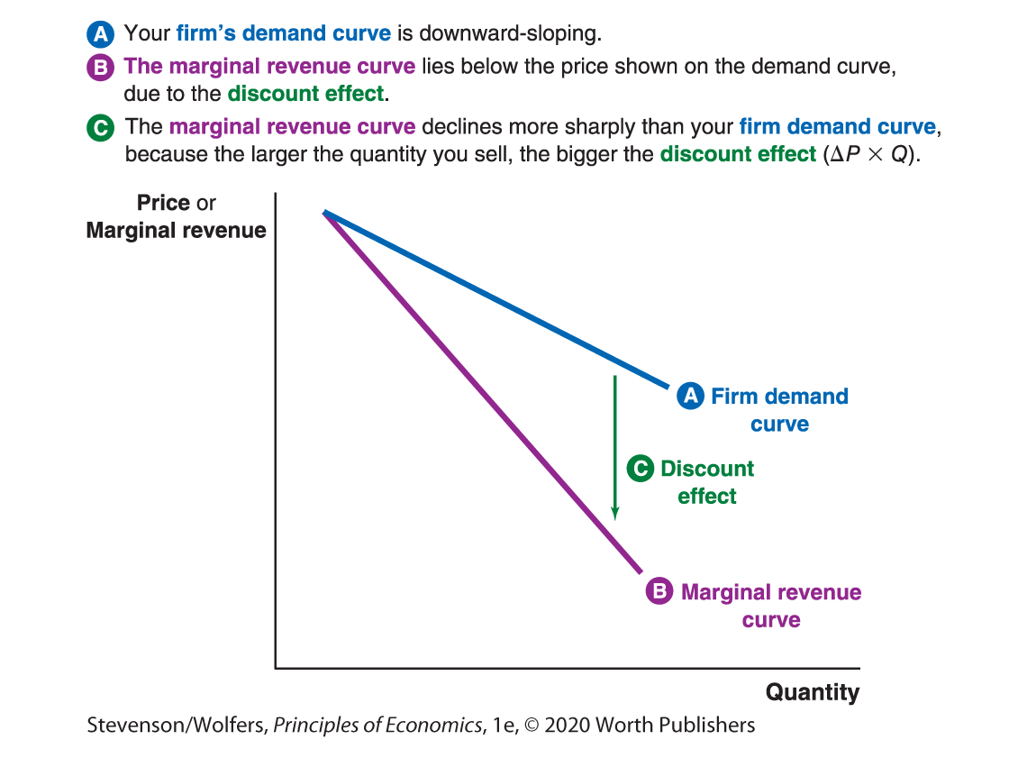
Figure 5 | Your Marginal Revenue Curve
Finally, and perhaps most importantly: Even though marginal revenue is related to your firm’s demand curve, don’t make the mistake of saying that they’re the same thing.
The Rational Rule for Sellers
Okay, so now it’s time to put yourself in Sofia’s shoes and make some business decisions. We’re going to do this in two steps as illustrated below in Figure 6. In step one, we’ll figure out what quantity to produce, and then in step two, we’ll figure out what price to charge.
(Study tip: Remember, first calculate the quantity to produce, and then figure out what price to charge. Why do things in this order? It’s simpler. While it’s possible to analyze the price first, it’s much more complicated.)
Step one: Keep selling until your marginal revenue equals your marginal cost.
So, how many cars should you sell? You should immediately recognize that this is a “how many” question, and simplify it using the marginal principle. It’s simpler to ask instead: Should I sell one more car? Now apply the cost-benefit principle, which suggests that yes, you should, as long as your marginal benefit from selling that car—which is the marginal revenue you’ll earn—exceeds (or equals) the marginal cost. That’s it! You’ve just discovered the Rational Rule for Sellers.
The Rational Rule for Sellers: Sell one more item if the marginal revenue is greater than (or equal to) marginal cost.
This a pretty intuitive rule. It says to sell another car if doing so will boost your revenue by at least as much as it boosts your costs. It follows that each car you sell will boost your profits. (When marginal revenue and marginal cost are exactly equal, your profits will neither increase nor decrease. The rule says to still sell that last item, mainly because it’ll make the rest of your analysis simpler.)
If you follow this rule and take every opportunity to sell cars when they’ll boost your profits, then you’ll keep selling until:
Marginal revenue = Marginal cost
You probably recognize this as a version of the Rational Rule that we discovered in Chapter 1, adapted to sellers. That rule said: If something is worth doing, keep doing it until your marginal benefits equal your marginal costs. Applying that idea to a seller, it says: If it’s profitable to sell cars, keep selling them until marginal revenue equals marginal cost.
In fact, this is the most important advice I can give any seller, so let me repeat it: To figure out what quantity to sell, keep selling until marginal revenue equals marginal cost. This occurs where the marginal revenue and marginal cost curves meet, as shown in Figure 6.
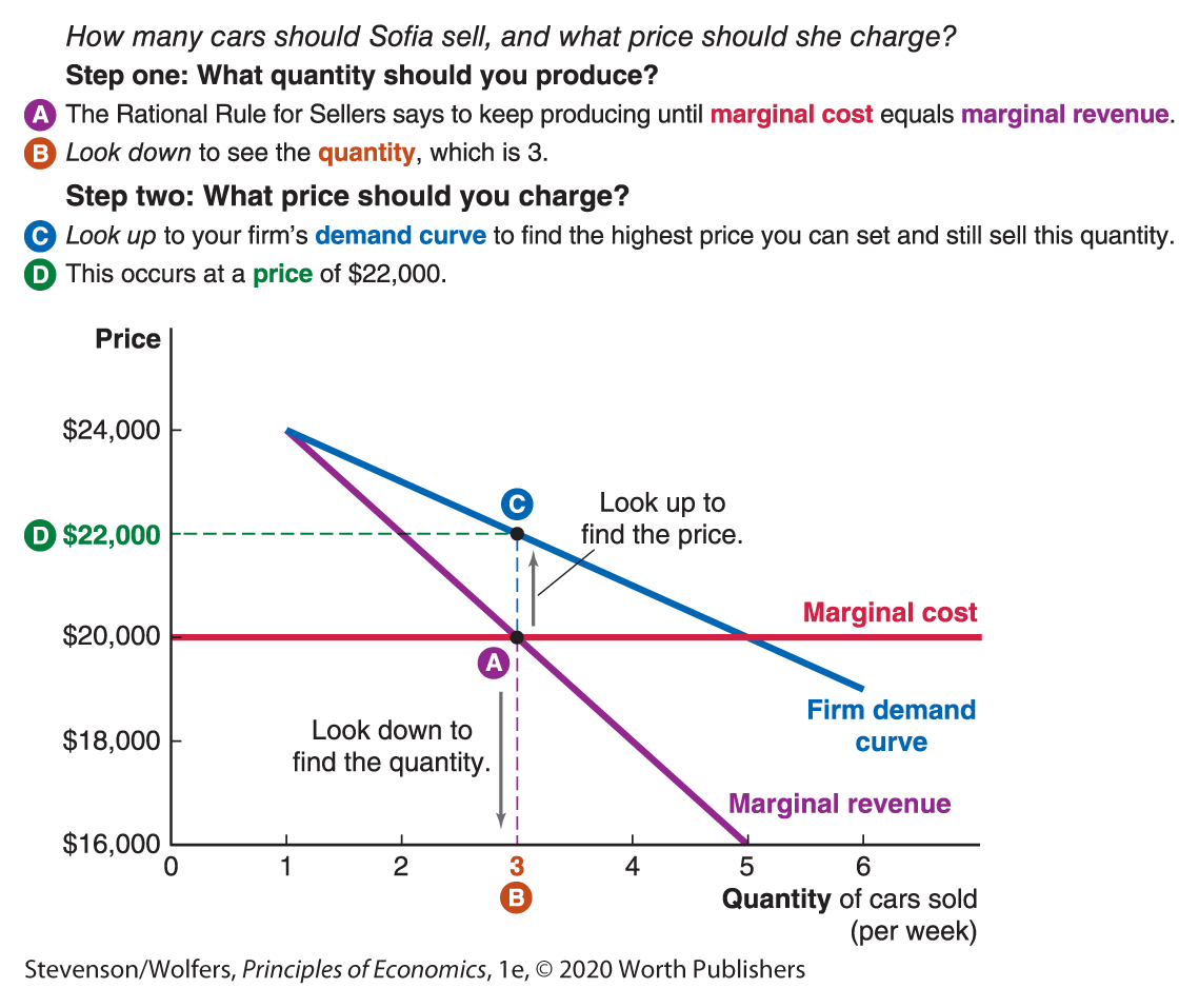
Figure 6 | Setting Prices and Quantities with Market Power
Step two: Set your price on the demand curve (not the marginal revenue curve).
OK, so we’ve figured out what quantity to produce. Now it’s time for step two, choosing what price to charge.
You should always charge the highest price you can, as long as you can sell the quantity you’ve decided on in step one. You can figure this out by looking at your firm’s demand curve: For the specific quantity you’ve decided to produce, look up to the firm demand curve to see what price to charge.
Be careful, because this is a step where students often make the mistake of just looking to see where the curves cross. You look to where marginal revenue and marginal cost cross to figure out the quantity to produce. Don’t make the mistake of looking at marginal revenue to figure out what price to charge. Rather, realize that the maximum price you can charge is all about what your customers are willing to pay. And so you should look up to the demand curve to see what price you can charge, given this quantity.
Here’s a simple memory trick to help you remember the two steps: Once you’ve found where marginal revenue cuts marginal cost, look down to see your quantity, and look up to find your best price.
OK, that’s it. You now know how you should set prices whenever your business has market power. Want proof that these two steps lead to the largest possible profit? Let’s work through Sofia’s profit and loss statement.
Do the Economics
Calculate the weekly profit that Sofia will make for each price and quantity combination. Her profit is simply her total revenue (Price × Quantity), minus total cost, which can be calculated by noting that each car costs her $20,000.

If Sofia follows the Rational Rule for Sellers, she will keep selling until her marginal revenue equals marginal cost, which occurs at a quantity of 3 cars. This decision leads her to earn a profit of $6,000 per week.
To confirm that this was the best decision, look at the final column, which shows the total profit that Sofia earns based on each alternative. Check and you’ll see that the Rational Rule for Sellers led her to the highest possible profit.
There’s one more fact worth noticing about Sofia’s decisions. If she cut her price even further to $21,000, then she would sell one more car. This implies that there’s a buyer out there who would get $21,000 worth of benefits from that car. But each car only costs Sofia $20,000. This suggests that selling one more car could make society better off. But Sofia chooses not to sell that fourth car, because it doesn’t make her better off. This illustrates a very important point: When businesses have market power, the market outcome does not maximize total economic surplus. To see that even more vividly, we’ll have to travel to Africa to see how market power nearly cost millions of people their lives.