29.2 Common Characteristics of Business Cycles
The novel Anna Karenina opens with the observation that “every unhappy family is unhappy in its own way.” The observation applies to unhappy economies too, as each recession is unique. Recessions vary in their causes, their duration, and their depth. The same thing is true of expansions, meaning that no two business cycles are ever the same.
While each business cycle is unique, they also tend to have some common features. Let’s take a look at what they are.
Recessions Are Short and Sharp; Expansions Are Long and Gradual
As you can see in Figure 8, a typical business cycle involves a short and sharp recession, followed by a long and gradual expansion. Since World War II, the average recession has lasted only one year, while the average economic expansion has lasted five years, reflecting the fact that an economic expansion could go on forever with the economy operating at potential. Recessions happen quickly and tend to involve steep declines in output and a sharp rise in unemployment. Expansions tend to be more gradual as the economy slowly recovers and grows. It can take years for the economy to heal and return to normal after a recession.

Figure 8 | Short, Sharp Recessions and Long, Gradual Expansions
Data from: U.S. Congressional Budget Office; Bureau of Economic Analysis.
The disruptions that cause an economy to go into recession are varied and have included slowing productivity, oil price hikes, credit controls, high interest rates, banking crises, overvaluation of technology stocks, a housing market meltdown, and a financial crisis.
The Business Cycle Is Persistent
Business cycle conditions are persistent, which means that it’s a reasonable bet that current conditions will continue in the near future. To illustrate this, Figure 9 plots the output gap in a given year against the output gap in the following year. If this year’s conditions were to always repeat themselves the next year, each dot would lie on the 45-degree line and the output gap would never change. The fact that most of the dots are clustered around the 45-degree line illustrates the fact that the output gap in any one year is typically similar to the output gap the next year. While the output gap does in fact change over time, these changes are both slow enough and unpredictable enough that your best prediction of next year’s output gap is simply this year’s gap. That’s why economists describe business cycles as persistent.

Figure 9 | Business Cycles Are Persistent
Data from: U.S. Congressional Budget Office; Bureau of Economic Analysis.
This tendency for current conditions to persist makes predicting the short term a lot easier! Many forecasters begin with an assumption that whatever happened this year is the best starting point for figuring out what will happen next year. So however the economy is performing this year is how it will likely perform next year.
The Business Cycle Impacts Many Parts of the Economy
The interdependence principle reminds us that the many different parts of the economy are interconnected. As a result, many economic variables move up and down together over the business cycle. This co-movement means that if one part of the economy is doing well, then other parts of the economy are probably also doing well. Likewise, if one part of the economy is doing badly, it’s likely that the same is true for other parts of the economy. Let’s see how.
Different states rise and fall together.
The business cycle also affects economic conditions in just about every state in the country, as shown in Figure 10.
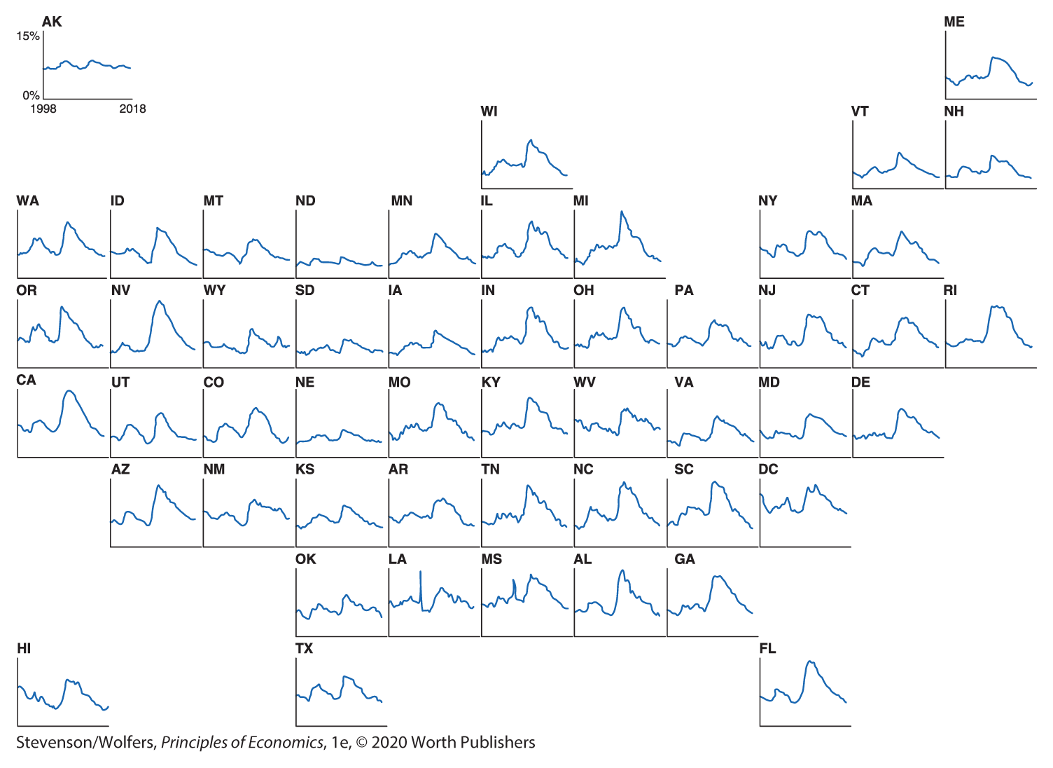
Figure 10 | State Unemployment Rates Rise and Fall Together
Data from: Bureau of Labor Statistics.
When a recession hits, the effects ripple across the country, as Ford produces fewer cars in Michigan, banks in New York make fewer loans, and families in Texas reduce their spending. And when there’s an economic expansion, it also affects every state. Find your state in Figure 10 and compare its unemployment rate with that in nearby states and the rest of the country. While there are some differences across states in how high unemployment goes, no state is immune from a recession.
Different economic indicators rise and fall together.
There are many different indicators that track economic activity, and they tend to move together. Figure 11 shows that if GDP is rising, then it’s also likely that industrial production is rising, retail sales are rising, and employment is rising. And it’s not just these indicators—the creation of new businesses, housing construction, automobile sales, imports from overseas, new investment projects, business profits and workers’ real wages, stock prices, inflation and interest rates—all tend to rise and fall with the business cycle. When we turn to analyzing macroeconomic data, you’ll learn the top 10 indicators that economy watchers track.

Figure 11 | Many Economic Indicators Rise and Fall Together
Data from: Bureau of Economic Analysis; Bureau of Labor Statistics; Board of Governors of the Federal Reserve System; Federal Reserve Bank of St. Louis.
Different industries rise and fall together.
The business cycle affects just about every sector of the economy. Figure 12 illustrates that whatever industry you’re in, a recession is usually bad for business, while an expansion is usually good for business. There’s an exception, and it’s not shown on the chart: The business cycle is really about the private sector, and so the public sector often follows a different pattern. That’s because the output of the public sector is determined by the political process rather than by market conditions. In addition, the demand for some government services tends to rise when the rest of the economy falls.

Figure 12 | Most Private-Sector Industries Rise and Fall Together
Data from: Bureau of Labor Statistics.
You’ll also notice that some sectors are more sensitive to business cycles than others. In particular, spending that’s easy to put off—like building a new house or buying a car—tends to rise and fall more strongly with business cycle swings.
Some variables lead the cycle, while others lag.
Leading indicators are variables that tend to predict the future path of the economy. Important leading indicators include business confidence, consumer confidence, and the stock market. Leading indicators help you get a better sense of where the economy is headed because they tend to change first. For example, consumers lose confidence in the economy before they start to substantially cut back their consumption.
Lagging indicators are variables that tend to follow business cycle movements with a bit of a delay. Unemployment tends to be a lagging indicator because managers who have invested in developing their staff are reluctant to make cutbacks until they’re convinced they’re really necessary.
Okun’s Rule of Thumb Links the Output Gap and the Unemployment Rate
Economic activity starts to increase at the end of a recession, but the economy will continue to have unused resources until the output gap is closed. One of those resources is workers, and so the unemployment rate moves in sync with the output gap. Figure 13 illustrates this relationship, showing that when output is below potential, unemployment tends to be high, and when output is above potential, unemployment tends to be low.
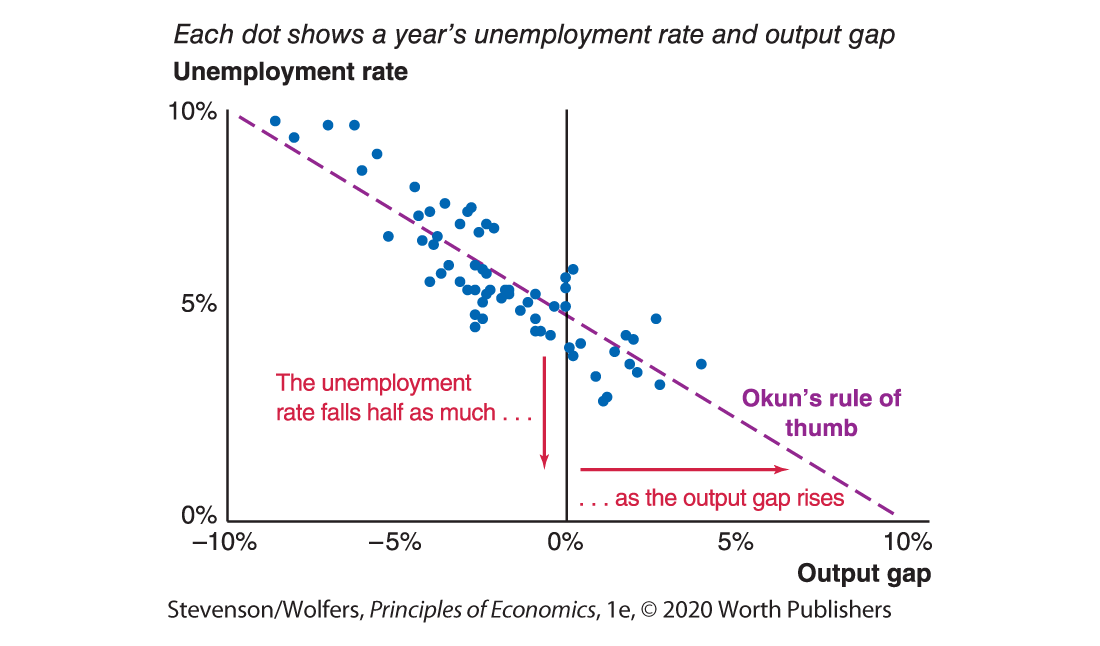
Figure 13 | Okun’s Rule of Thumb Links Unemployment and GDP
Data from: Bureau of Economic Analysis; Bureau of Labor Statistics.
When output is at potential, the unemployment rate is equal to the equilibrium unemployment rate. You learned in Chapter 23 that the equilibrium unemployment rate is the unemployment rate that the economy tends to return to over time, and it occurs when the economy is operating at potential. The equilibrium unemployment rate isn’t zero because of both frictional and structural causes of unemployment. Indeed, over the past century the equilibrium unemployment rate in the United States has averaged around 5%.
Okun’s rule of thumb quantifies the relationship between output and the unemployment rate. It says that for every percentage point that actual output is less than potential output, the unemployment rate will be around half a percentage point higher. For instance, if you project the output gap will decline from zero to −2%, the unemployment rate will likely rise by about 1 percentage point, from, say, 5% to 6%.