30.2 The IS Curve: Output and the Real Interest Rate

Learning Objective Use the IS curve to analyze the relationship between the real interest rate and equilibrium GDP.

The most important price in the economy.

The real interest rate may be the most important price in the economy because it represents the opportunity cost of spending. The opportunity cost principle tells you that before spending money, you should ask, “Or what?” You can spend money now, or you can save it, earn interest, and buy even more in the future. The real interest rate, denoted by r, tells you how large this opportunity cost is—how much more stuff you’ll be able to buy if you wait until next year. So, the real interest rate—which is the nominal interest rate adjusted for inflation—is the price that determines this year’s aggregate expenditure.

The real interest rate is also critical because it’s one of the levers policy makers use to influence the economy. The Federal Reserve raises the interest rate—which increases the opportunity cost of spending—when it wants to induce people to spend less. And when the Fed wants to stimulate more spending, it reduces the interest rate, which reduces the opportunity cost of spending money today. As such, careful adjustments to the real interest rate can help offset booms and busts.

These insights inform the roadmap ahead. Our goal is to develop a comprehensive framework for understanding how interest rates affect the economy and why rates rise and fall. We’re going to proceed in two steps. First, we’ll figure out how the real interest rate affects GDP—a relationship that we’ll call the IS curve. Second, we’ll assess how changing financial conditions determine the real interest rate, summarizing our findings in a line we’ll call the MP curve. Putting them together will yield a framework you can use to analyze changes in economic conditions. And if you’re puzzled about how these two curves got their names, don’t worry, we’ll also get to that.

Aggregate Expenditure and Interest Rates

Before we can get there, we need to lay the foundation, analyzing how the real interest rate affects aggregate expenditure. We’ll do this by separately exploring how the real interest rate shapes each of the components of aggregate expenditure: consumption, planned investment, government purchases, and finally, net exports. (We explored some of these themes in greater detail in Chapters 25–28 so we’ll just hit the key ideas here.)

Lower interest rates boost consumption.

The graph plots real interest rate from 0 to 4 percent against consumption shows a downward sloping curve. The accompanying equation shows that decreased r leads to increased C.

The real interest rate is central to your spending decisions as a consumer because of the opportunity cost principle: You can save and earn interest on any income you don’t spend. As a result, the real interest rate represents the opportunity cost of boosting this year’s consumption spending. The lower the real interest rate is, the lower this opportunity cost. That’s why a low real interest rate leads to more consumption.

The real interest rate is also the cost of borrowing. If you need a loan in order to buy a car, a house, or some other big-ticket item, your bank will charge you interest. The lower the real interest rate is, the less you’ll have to repay your bank, which is another reason that low interest rates lead people to increase their spending on big-ticket items.

Note, however, that there’s one group for whom a low real interest rate will reduce consumption, and that’s people who rely on interest payments for their income. In their case, lower interest rates translate into less income, which can lead them to cut back on their consumption spending. While this describes some people (particularly retirees), across the whole economy this effect is relatively small. And so, on average, lower interest rates lead to more consumption.

Lower interest rates boost investment.

The graph plots real interest rate from 0 to 4 percent against investment and it shows a downward sloping curve. The accompanying equation shows that decreased r leads to increased l.

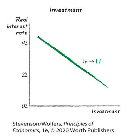
For businesses considering capital investments, the real interest rate is important, again because of the opportunity cost principle: If you spend your money buying new equipment or structures, you can’t put that money in the bank to earn interest. And so the opportunity cost of investing in new capital is lower when real interest rates are lower. As a result, low real interest rates lead to more investment spending. Indeed, a low enough interest rate can be the difference that makes billions of dollars of investment projects worth pursuing, which is why investment is particularly sensitive to the real interest rate.

Lower interest rates boost government purchases.

The graph plots real interest rate from 0 to 4 percent against Government purchases and it shows a downward sloping curve. The accompanying equation shows that decreased r leads to increased G.

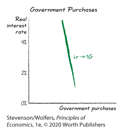
Low interest rates reduce the cost of interest payments on government debt. These interest payments—which are a transfer from the government to those it borrows from—don’t directly affect aggregate expenditure. But low interest payments mean that there’s more money left in the government budget for spending on roads, bridges, and other forms of aggregate expenditure. As a result, lower interest rates can lead to an increase in government purchases, particularly for state governments, which are often required by law to balance their budgets. Low interest rates don’t always spur more government purchases though, because governments might use their extra funds to pay down their debt instead.

Lower interest rates boost net exports.

The graph plots real interest rates from 0 to 4 percent against net exports and shows a downward sloping curve. The accompanying equation shows that decreased r leads to decrease in U.S. dollar which in turn leads to decrease in net exports.

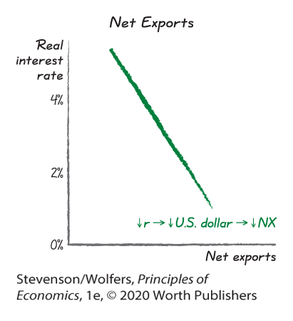
Net exports also depend on the real interest rate, but through an indirect mechanism: Low interest rates make the U.S. dollar cheaper, and this increases net exports (which is exports less imports). Let’s take each of these steps in turn.

A low real interest rate in the United States leads international money managers to send their funds to other countries that offer better returns. This means they’ll demand fewer U.S. dollars, leading the dollar to become cheaper. So the initial effect of a lower interest rate is that it takes fewer yen, euros, or yuan (the currencies of Japan, Europe, and China) to buy an American dollar.

This cheaper dollar increases exports and reduces imports. Start by considering exports: An American-made car that costs US$10,000 (“US$” means “in U.S. dollars”) now sells for fewer yen, euros, or yuan than it did before. This effective price cut leads foreigners to buy more of our exports. As a result, spending on our exports rises. Next, consider imports: A cheaper dollar means that it now takes more U.S. dollars to buy a €10,000 car (the € sign means “euros”). This effective price rise leads Americans to buy fewer imports. If the quantity of imports declines by enough to offset the higher prices, then total spending by Americans on imported goods will also fall. Put these effects together, and lower real interest rates lead to a cheaper U.S. dollar, causing exports to rise and imports to fall, and hence higher net exports.

The IS Curve Describes the Link Between the Real Interest Rate and the Output Gap

Let’s summarize what we’ve found so far. We discovered that a decrease in the real interest rate leads to an increase in every component of aggregate expenditure, boosting consumption, investment, possibly government purchases, and net exports.

The flow diagram shows that a decrease in the real interest rate leads to an increase in C, an increase in I, an increase in G, and an increase in net export. The accompanying text reads, the real interest rate is the opportunity cost of spending money this year (rather than next).

Of these effects, the boost to investment is usually the most important because investment—both in machinery and housing—is particularly sensitive to the interest rate.

Lower interest rates boost aggregate expenditure.

The top row of Figure 3 shows that consumption, investment, government purchases, and net exports are each higher when the real interest rate is lower. The bottom row simply adds these up to illustrate that aggregate expenditure—which is the sum of each of these forms of spending—is higher when the real interest rate is lower.

Figure 3 | The Real Interest Rate and Aggregate Expenditure

The first graph plots consumption against r and depicts a downward-sloping curve that extends along C subscript r equals 4 percent and C subscript r equals 2 percent. The second graph plots planned investment against r and depicts a downward-sloping curve that extends along I subscript r equals 4 percent and I subscript r equals 2 percent. The third graph plots government purchases against r and depicts a downward-sloping curve that extends along G subscript r equals 4 percent and G subscript r equals 2 percent. The fourth graph plots net exports against r and depicts a downward-sloping curve that extends along N X subscript r equals 4 percent and N X subscript r equals 2 percent.

The resulting fifth graph plots aggregate expenditure against real interest rate, r and depicts a downward-sloping curve that extends along C subscript r equals 4 percent plus I subscript r equals 4 percent plus G subscript r equals 2 percent plus N X subscript r equals 4 percent and C subscript r equals 2 percent plus I subscript r equals 2 percent plus G subscript r equals 2 percent plus N X subscript r equals 2 percent.

Text reads, Lower real interest rates yield more consumption, investment, government purchases, and net exports which implies that lower real interest rates yield higher aggregate expenditure.

This insight—that a lower real interest rate will boost aggregate expenditure—is central to the framework we’re developing. We summarize this finding as:

The flow diagram shows that a low real interest rate leads to increased C, I, G, and N X which leads to an increase in aggregate expenditure. An equation reads, aggregate expenditure equals C plus I plus G plus N X.

A rise in aggregate expenditure is matched by a rise in production and hence GDP.

Recall our previous finding that businesses adjust their output to meet demand, so that output adjusts until it’s equal to aggregate expenditure. As a result, a lower real interest rate which boosts aggregate expenditure will increase the level of GDP:

The flow diagram shows that a decrease in real interest rate leads to an increase in C, I, G, and N X resulting in increased aggregate expenditure that in turn leads to increased G D P. The accompanying text reads, Businesses adjust output to meet demand so in equilibrium: G D P equals Aggregate expenditure

Finally, potential output is determined by long-run factors that are unaffected by these business cycle changes. Since potential output is unchanged, the interest-rate-induced increase in output also increases output relative to potential output, leading to a more positive output gap.

The flow diagram shows that a low real interest rate leads to an increase in C, I, G, and N X which leads to an increase in aggregate expenditure that causes G D P to increase resulting in an output gap. The accompanying text reads Potential G D P is unchanged so changes in G D P translate to change in the output gap.

The IS Curve illustrates the link between interest rates, GDP, and the output gap.

That’s it! We’ve uncovered the link by which lower real interest rates lead to higher real GDP and a more positive output gap.

Figure 4 shows this relationship by graphing the IS curve, which illustrates how lower real interest rates lead to more spending and hence more output and a more positive output gap. It’s called the IS curve because it describes Investment and Spending decisions. And it illustrates the Interest Sensitivity of output. (Historically, it was called the IS curve because Investment is the key form of interest-sensitive spending, and Saving is used to fund investment.)

IS curve

Illustrates how lower real interest rates raise spending and hence GDP, leading to a more positive output gap.

Figure 4 | The IS Curve

The introductory text reads:

The I S curve illustrates that a lower real interest rate leads output to be larger, relative to potential output.

A The real interest rate is on the vertical axis.

B The output gap, which goes on the horizontal axis, measures output relative to potential G D P.

C The I S curve is downward-sloping, because lower real interest rates boost aggregate expenditure, which leads to a higher level of G D P and, hence, a more positive output gap.

The graph plots B output gap (real G D P relative to potential G D P) ranging from negative 10 percent to 5 percent against A real interest rate ranging from 0 to 6 percent. The downward sloping curve extends between (negative 9.8, 5.8) and (4.9, 1) and is labeled C I S curve.

You construct the economy’s IS curve by adding up the level of aggregate expenditure at each real interest rate. Because output adjusts to the level of aggregate expenditure, this also reveals the level of GDP, and then it’s just a matter of comparing GDP to potential GDP to calculate the corresponding output gap. Calculate this output gap when the real interest rate is 1%, 2%, 3%, and so on, then connect these dots, and you’ve estimated the IS curve.

The IS curve is like a macroeconomic demand curve.

You are probably used to thinking about a demand curve as showing this year’s demand for a specific product, like gas. In many ways, the IS curve is similar—it shows this year’s demand for all types of output and so you can think of it as showing the macroeconomic demand for output.

The graph plots output gap against real interest rate and depicts a downward sloping curve labeled I S curve. An arrow points to the vertical axis labeled real interest rate and the accompanying text reads, It’s a price, so it goes on the vertical axis. An arrow points to the horizontal axis labeled output gap and the accompanying text reads, It’s a quantity so it goes on the horizontal axis.

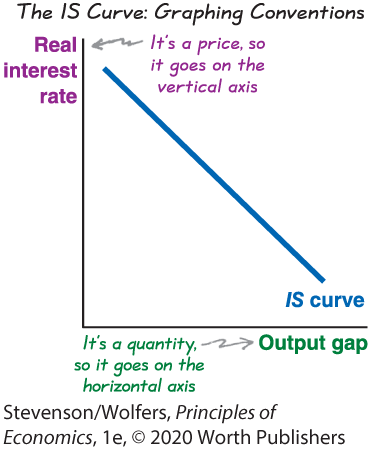
As with a demand curve, the vertical axis shows a price—in this case, that price is the real interest rate, which is the opportunity cost of spending money this year rather than next. And the horizontal axis shows the corresponding quantity—the output gap—which is the total quantity of goods and services purchased across the whole economy, relative to potential output.

The IS curve is downward-sloping, like a typical demand curve.

That’s because a lower real interest rate decreases the opportunity cost of making purchases this year, leading people across the whole economy to respond by buying more goods and services. Or you can say this the other way: The higher the real interest rate is, the greater the opportunity cost of buying stuff this year (rather than next), and so the smaller the quantity of stuff people demand this year. And while we call the IS curve a curve, as Figure 4 illustrates, it could also be a straight line.

How to Use the IS Curve

The IS curve is a valuable tool for forecasting economic conditions. For instance, can you forecast what the output gap will be if the real interest is 4%?

The graph plots output gap that increases along the horizontal axis from left to right against the real interest rate that decreases along the vertical axis from top to bottom. The downward sloping curve is labeled I S curve and the accompanying text reads, A lower real interest rate … leads to higher output gap.

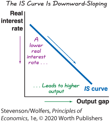
Figure 5 illustrates how to figure this out. First, locate the 4% real interest rate on the vertical axis. Then look across until you find the IS curve. Now look down to discover that the corresponding level of GDP is 5% below its potential level. That’s it, you’ve now got your forecast.

Figure 5 | Changing Interest Rates Leads to a Movement Along the IS Curve

The graph plots output gap in percent (G D P relative to potential G D P) against real interest rate. The graph shows a downward sloping curve C with the points A (negative 5, 4); B (2.5, 1). Dashed lines connect the point A and B to vertical axis and horizontal axis.

The accompanying text reads as follows:

A When the real interest rate is 4%, the output gap is negative 5%

B When the real interest rate is 1%, the output gap is 2.5%

C Changes in the real interest rate lead to a movement along a fixed I S curve.

If other things change, so should your forecast.

Of course, this is your forecast, holding other things constant. If other factors change, then so should your forecast. This points to another way the IS curve can be helpful: You can use it to forecast the consequences of changing economic conditions.

A change in the real interest rate leads to a movement along the IS curve.

In Figure 5, you started by looking at point A, where the real interest rate is 4%. Now consider what happens if policy makers cut the real interest rate to 1%. Locate the new 1% real interest rate on the vertical axis and look across until you hit the IS curve. Look down, and you’ll see that it corresponds to an output gap of +2.5%, which means that GDP will be 2.5% above potential GDP. And so you can conclude that reducing the real interest rate from 4% to 1% will cause the output gap to change from −5% to +2.5%.

Notice that this change in the real interest rate led the economy to move from one point on the IS curve to another point on the same curve. This makes sense: The point of the IS curve is to illustrate how the output gap responds to changes in the real interest rate, and so changes in the real interest rate lead to a movement along the IS curve.

This is where it’s important that you distinguish between:

• Changes in the real interest rate: which cause a movement along the IS curve
• Changes in other factors that change aggregate expenditure at a given interest rate: which cause the IS curve to shift

Later in the chapter, we’ll look at the changes in other factors that can shift the IS curve.

Interpreting the DATA

What caused the early 1980s recession?

Builders got creative when it came to lobbying for lower interest rates in the 1970s.

In 1979, newly appointed Federal Reserve Chair Paul Volcker pledged to eliminate the double-digit inflation that was then plaguing the U.S. economy. He figured that if he engineered an economic slowdown, inflation would fall, as businesses rarely raise their prices when the economy is weak.

To create this slowdown, the Federal Reserve jacked up the interest rate. At its peak, the nominal interest rate was 20%, and the real interest rate was as high as 10%. Just as our analysis suggests, a high real interest rate led businesses to sharply curtail investment spending, households to cut back on consumption, and it caused the U.S. dollar to rise, leading net exports to fall. Aggregate expenditure fell, causing GDP to decline.

The recession deepened, and protests mounted. Indebted farmers blockaded the Federal Reserve building with their tractors; construction workers mailed their complaints on pieces of lumber, and car dealers sent the Fed coffins containing the keys of unsold cars. A Texas congressman threatened to impeach Volcker.

High real interest rates ended up being too successful at slowing the economy. GDP fell to be far below potential output, which created a very negative output gap. The unemployment rate rose from under 6% in 1979 to a peak of nearly 11% in 1982. This episode settled any remaining debate about the importance of the real interest rate in shaping the business cycle. It vividly demonstrated the relevance of the IS curve, as this bout of high interest rates led to lower levels of aggregate expenditure, lower GDP, and a sharply negative output gap.

At this point, you’ve got a good handle on the IS curve: It tells you what the output gap will be at each real interest rate. But what determines the real interest rate, and what could cause it to change? Figuring that out is our next task.