30.4 The IS-MP Framework
Okay, let’s put it all together. The IS curve illustrates how the output gap depends on the real interest rate. And the MP curve tells you what the real interest rate will be. Put them together, and you’ll have a complete story of what determines the state of the economy. As a manager and as an investor, you’ll be able to use this framework to interpret economic news and figure out what it means for your future.
IS-MP Equilibrium
We bring the IS and MP curves together in Figure 8. As you know, the IS curve shows you the level of the output gap that corresponds with each possible value of the real interest rate. The MP curve tells you what the real interest rate is. Their intersection determines the macroeconomic equilibrium, revealing the level of the output gap that’s consistent with the real interest rate. In this example, the risk-free interest rate plus the risk premium sets the real interest rate at 4%, which yields an equilibrium GDP that is 5% below its potential level, for an output gap of 

Figure 8 | The IS-MP Framework
That’s it—you’ve got your forecast for economic conditions. More than that, you’ve now put together a comprehensive framework for understanding business cycles. This isn’t just a textbook exercise—this is the framework that guides the macroeconomic forecasts produced by many government policy makers, Wall Street investors, and business analysts.
Fluctuating Demand and Business Cycles
So far, we’ve seen that aggregate expenditure plays a central role in determining the macroeconomic equilibrium. This suggests that perhaps we can understand recessions and depressions as periods of weak or declining aggregate expenditure. By this view, the booms and busts of the business cycle reflect the economy shifting between periods of strong and weak demand. We explore this idea in Figure 9, which illustrates two alternative macroeconomic equilibria.
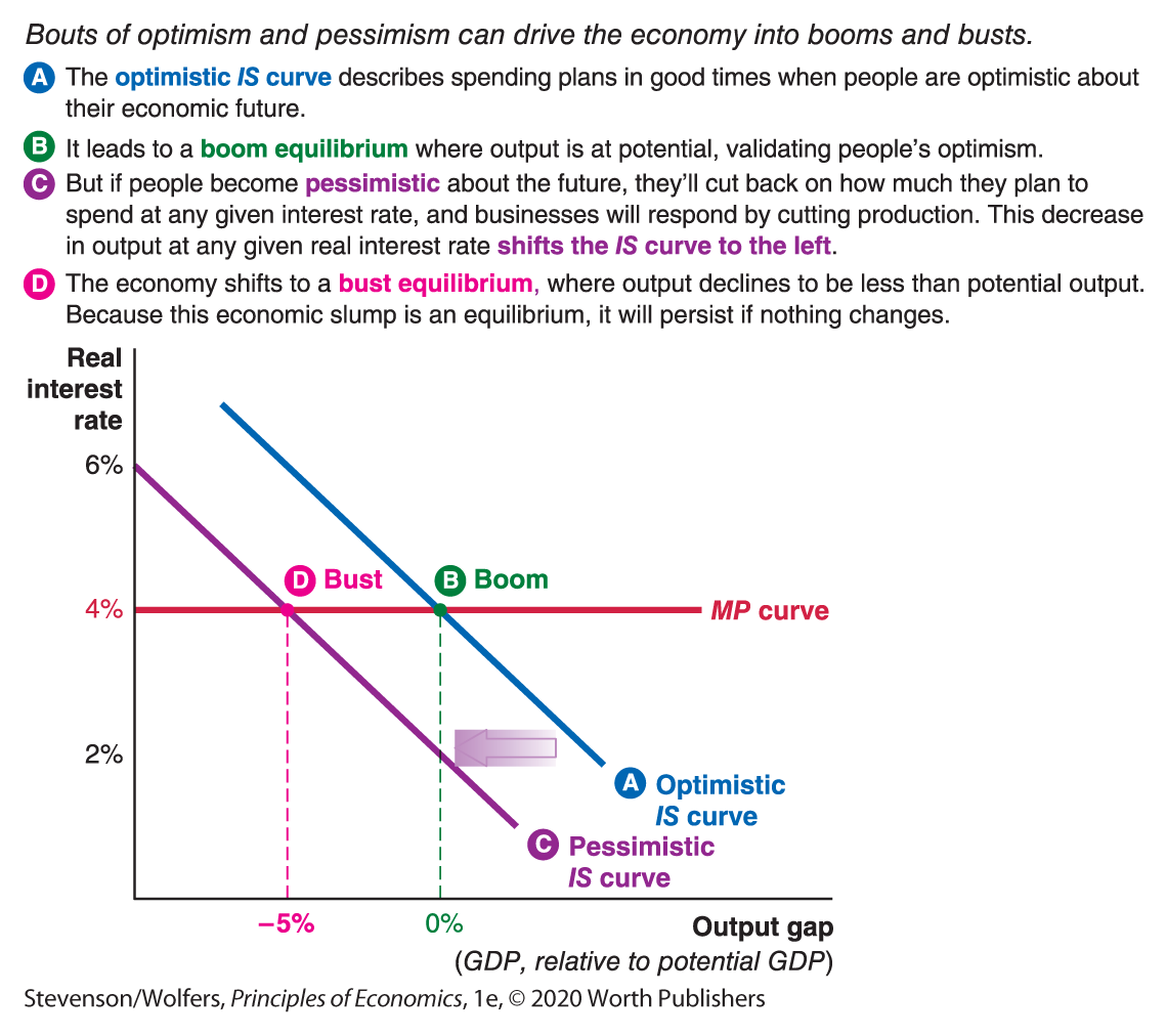
Figure 9 | Booms and Busts
Strong aggregate expenditure leads to a booming economy and full employment.
One possibility is that people are optimistic about the future. Students who are optimistic that they’ll get a good job after graduation will spend more money at any given interest rate, as will workers who are optimistic about promotions and pay raises, and so will entrepreneurs who are confident about their business success. These optimistic spending plans are illustrated by the blue IS curve in Figure 9, which shows high levels of aggregate expenditure at each level of the real interest rate. This leads to a macroeconomic equilibrium with an output gap of zero, which means that GDP is at its highest sustainable level. In this booming economy, output is high, unemployment is low, and the economic outlook is sunny enough that continued economic optimism is warranted. Think of this as the macroeconomic equilibrium in good times.
Insufficient spending can lead to an economic slump and unemployment.
There’s also the possibility that a wave of pessimism hits. Pessimism about future economic conditions might lead consumers to cut back on their spending, or businesses to cut back on their investment plans. In each case, the result is a decrease in aggregate expenditure at any given real interest rate and level of income, which causes the IS curve to shift left to the purple line.
This lower level of aggregate expenditure yields a new macroeconomic equilibrium at a much lower level of GDP. The output gap is now negative, which means that the economy is producing below its potential. Because businesses are producing less, they need fewer workers. As a result, in this recessionary equilibrium, people have lower incomes, and there’s widespread unemployment. In this new equilibrium, the pessimism that caused the downturn now appears to be warranted. Pessimism about an economic slump has caused an economic slump. Think of this as the equilibrium during the Great Depression, or in any of the downturns since.
Changes in aggregate expenditures create macroeconomic fluctuations.
In this analysis, the economy fluctuates between periods of boom and bust—and points in between—due to changes in aggregate expenditure shifting the IS curve. While we’ve focused on what happens when spending changes due to bouts of optimism or pessimism, similar booms and busts will follow in response to any factor that causes aggregate expenditure to shift at a given interest rate. The broader lesson is that many of the ups and downs of the business cycle reflect shifts in aggregate expenditure.
Interpreting the DATA
Tracking waves of optimism and pessimism
By this view, the key to understanding changing business conditions is to keep track of changing spending patterns. If your business sells mainly to consumers, then surveys of consumer confidence can help you keep track of changing consumption plans. If your business sells machinery and investment goods to other companies, then surveys of business confidence can help you keep track of their spending plans. As Figure 10 shows, the economy does indeed appear to experience periods of optimism and pessimism.

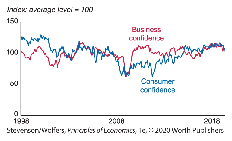
Figure 10 | Consumer Confidence and Business Confidence
Data from: University of Michigan Index of Consumer Sentiment and ISM Purchasing Managers Index.
Recessions can be individually rational and collectively terrible.
Many of these ideas about the possibility of deficient demand causing recessions were first put forward (in somewhat different terms) by economist John Maynard Keynes in the wake of the Great Depression, the worst economic slump in modern memory. The Depression shook the faith of many economists, leaving them wondering how it’s possible for the economy to perform so poorly as to leave millions of people unemployed. Amid this deep and prolonged downturn, Keynes argued that the economy can be in macroeconomic equilibrium even when output is far below its potential and unemployment is widespread. In doing so, he argued that unless the government intervened, an economic slump could persist for years.
The economic slump we outlined in Figure 9 illustrates the modern form of his argument. It illustrates a macroeconomic equilibrium in which the economy produces less than its potential. If nothing changes, a prolonged recession will follow. That’s because once we’re in this bad equilibrium, there’s no reason for either buyers or sellers to change their plans. After all, businesses cut back on production because people spend less, and people spend less because they’re worried about a prolonged recession.
This highlights the paradox of recessions: Each person is individually making the best decision they can, but those decisions add up to a collectively terrible outcome in which the economy is stuck in a bad equilibrium. The depressing lesson is that there’s no guarantee that businesses will produce enough to keep everyone employed.
EVERYDAY Economics
How the economy is just like a concert

It’s just like widespread unemployment.
If you want to better understand how recessions happen, think of the U.S. economy as being like a concert. In a concert economy, your butt is an employer, and your seat is a worker. If you sit down, your seat is fully employed, but if you stand up, your seat is unemployed. How do you decide what to do? The interdependence principle dictates that your best choice depends on what others do. At the concert, you’ll stay seated if all your neighbors are sitting down. In this equilibrium every seat is fully employed. But if your neighbors stand up, you’re better off standing too, because that’s the only way you’ll be able to see. When you stand, then others might also have to stand. The result is an equilibrium in which many seats are unemployed. I bet you’ve been at a concert that switches between the equilibrium in which all seats are employed, to one in which thousands are unemployed.
The same thing happens in the economy: You’ll employ plenty of workers at your business if there are plenty of customers willing to buy your products. But the number of customers willing to buy your products depends on how many workers other companies employ. Just as you’ll be forced to stand at a concert if others stand, you might be forced to fire some workers if your customers lose their jobs as other companies cut their payrolls. The concert economy can quickly shift from an equilibrium in which every seat is employed by someone to a different equilibrium in which many seats are unemployed, and so too the macroeconomy can shift from the good equilibrium in which every worker has a job, to a bad equilibrium in which millions of workers are unemployed.
Importantly, neither unemployed seats nor unemployed workers are inevitable. At the concert, if everyone else can be persuaded to sit down, you’ll also sit down, and the seats will be fully employed again. Likewise, in the economy, if people can be persuaded to spend money again, then businesses will increase their production to keep up, and they’ll hire the unemployed workers. In fact, as we’ll explore shortly, this is precisely how policy makers try to kickstart the economy out of recession.
Let’s now see how you can use this framework to understand the effects of macroeconomic policy.
Analyzing Monetary Policy

Yet another meeting, as the situation worsens.
Late 2008 was the apex of one of the most tumultuous periods in America’s economic history. House prices tumbled, the stock market plummeted, and every day seemed to bring news of another financial institution in danger of going bust. Businesses stopped investing, consumers cut their spending, and millions of people lost their jobs. The economy was in free fall, and no one knew how bad things could get. Was the next Great Depression just a few months away?
The pressure on policy makers to provide a fix was intense. Economists met with members of Congress and Federal Reserve officials, often in meetings lasting deep into the night. Some slept on their couches; others returned home for a shower and a change of clothes before returning to work—only to find that the situation had gotten even worse: The crisis had spread to other sectors of the economy, and to other countries. Fear was contagious, and it threatened to bring the whole economy down.
By the end of the year, GDP was well below potential GDP. These aren’t abstract statistics; they summarize a landscape littered with dormant factories, millions of jobless workers, and families doing without. If you were a member of the Federal Reserve or the President’s economic team, what would you do?
Monetary policy shifts the MP curve.
Policy makers at the Federal Reserve responded quickly and decisively, cutting its benchmark interest rate seven times over the course of 2008. It’s rare to see the Fed act this boldly. What did this mean for the economy, and for businesses? Fortunately, you can use the IS-MP framework to figure this out.
When the Fed changes the real interest rate, it shifts the MP curve. In this case, the Fed cut the interest rate, which shifted the MP curve down. As Figure 11 illustrates, this shift in the MP curve leads to a new equilibrium, which involves higher GDP at a lower real interest rate. Armed with this analysis, savvy managers realized they no longer needed to keep cutting back. Indeed, consistent with the forecast from our IS-MP analysis, the Fed’s dramatic actions halted the economy’s nosedive, and eventually there were signs that the worst days were behind us.

Figure 11 | Changes in Monetary Policy Shift the MP Curve
But it also became increasingly clear that monetary policy alone could not cure all of the economy’s ills. There came a time when the Federal Reserve had effectively cut the interest rate to zero, but the economy was still underperforming. It couldn’t cut the interest rate any further, because once rates are zero, there’s no longer any incentive to loan money rather than to store it in a safe. Even if further rate cuts were possible, they would have little or no effect. Yet it was clear that further action was required.
Analyzing Fiscal Policy and the Multiplier
The government can also influence the economy through fiscal policy—that is, by adjusting its own spending and tax policies. And so in 2009, the federal government passed a stimulus bill called the American Recovery and Reinvestment Act, which both increased government purchases and reduced some taxes. All told, this law—which created a burst of new spending on infrastructure, education, health, and renewable energy—was expected to cost around $787 billion, or a bit more than $2,500 per American.
When the federal government adjusts fiscal policy, it shifts the IS curve. In this case, an expansionary fiscal policy boosts aggregate expenditure, which shifts the IS curve to the right. Figure 12 shows that this expansionary fiscal policy leads to a rise in output and hence a more positive output gap. But to see how big this effect is, we need to explore an idea called the multiplier.
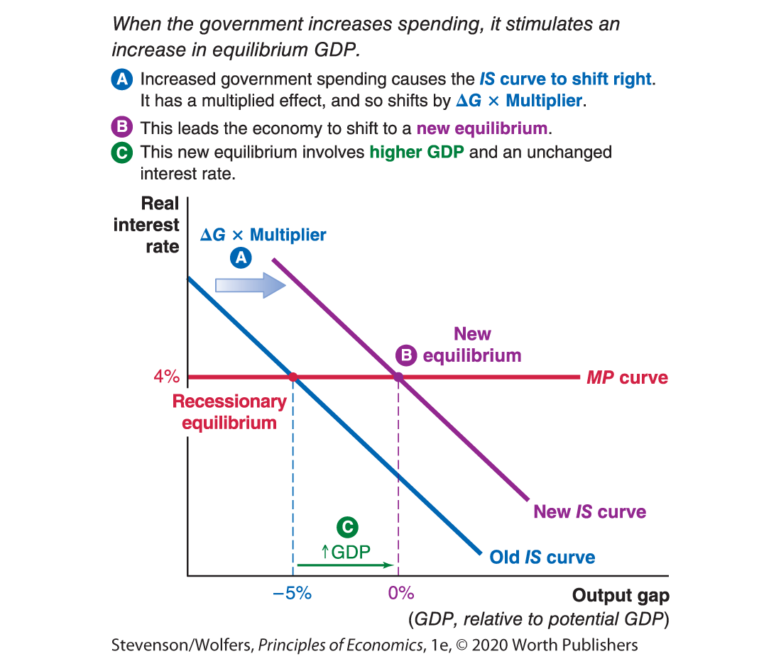
Figure 12 | Changes in Fiscal Policy Shift the IS Curve
An increase in spending has a multiplied effect on aggregate expenditure.
An initial burst of government spending will have repercussions throughout the economy. Consider the money spent building new roads. The direct effect is that unemployed transportation engineers, construction workers, and road maintenance crews will be hired and put to work. There will also be important ripple effects. For instance, a worker who decides to spend some of their earnings on a new car boosts the incomes of Ford workers and shareholders. There are also second-round ripple effects. As Ford sells more cars, it’ll hire more production workers, who might buy lunch at a local Subway, leading the franchise owner to hire more sandwich artists. There are third-round effects, too. If the new Subway staff buy clothes, the owner of the nearby clothing store also receives a boost to their income. And so it continues.

An initial boost in spending reverberates through the economy.
As this initial boost in spending reverberates through the economy, it illustrates the importance of the interdependence principle for understanding macroeconomic developments. This interdependence arises because one person’s spending is another person’s income. It means that extra spending by the government stimulates extra spending by construction workers, which stimulates extra spending in the car, food, and clothing industries. As the initial burst of government purchases ripples through the economy, it has a multiplied effect, leading to an even larger boost to aggregate expenditure.
The multiplier summarizes the effect of an initial burst of spending on output.
You can summarize the consequences of a rise in spending—including both the direct impact and the many rounds of subsequent ripple effects—with a single number called the multiplier. The multiplier measures how much GDP changes as a result of both the direct and indirect effects flowing from each extra dollar of spending. For instance, if the multiplier is 2, then an initial $1 boost to spending will generate a total of $2 in additional spending and hence output. When people have a greater propensity to spend any additional income they receive, the ripple effects of an initial burst of spending will be larger, leading the multiplier to be larger.
The multiplier is useful, because you can use it to forecast the effects of changes in spending as follows:

You can use the multiplier to figure out the likely consequences of the 2009 stimulus bill. (To simplify, we’ll treat the entire $787 billion cost of the stimulus bill as if it were a rise in government purchases, which is not strictly accurate.)
Do the Economics
How much will GDP rise after a $787 billion increase in government purchases, if the multiplier is 2?

If you want to dig more deeply into the logic (and math) of the multiplier, turn to the appendix titled “A Closer Look at Aggregate Expenditure and the Multiplier.”
The multiplier determines how far the IS curve shifts.
The multiplier is relevant to our IS-MP analysis because it determines how far the IS curve shifts following an initial burst of spending. The new IS curve shifts to reflect the new level of aggregate expenditure, and so it needs to account for both the direct effect of new spending and its ripple effects stimulating yet more spending. As a result, Figure 12 illustrates the IS curve shifting by an amount equal to the initial change in spending times the multiplier. This shift in the IS curve leads to a new equilibrium, which involves higher GDP, but no change in the real interest rate.
This analysis tells you that fiscal stimulus will help the economy grow, and so managers should get ready to increase production. In fact, the economy largely followed this forecast, as the 2009 fiscal stimulus bill was an important factor leading to a stronger economy in 2010 and 2011.