31.3 The Phillips Curve
A strong economy has created a rather pleasant dilemma for you and your fellow executives at Outback Steakhouse. Folks have healthy incomes, and so millions more people are willing to splurge to enjoy a steak dinner. But it’s a dilemma because Outback Steakhouses are already overflowing, and in many cases, customers are forced to wait for over an hour for a table. Some customers give up waiting and leave. Outback Steakhouse faces excess demand given its limited seating capacity, as the quantity demanded at the prevailing price exceeds the quantity that it can supply.
In the long run, if business continues to boom, it’s worth building more restaurants. But in the short run, you’re stuck with your existing capacity. In this situation, what advice would you give your fellow executives?
Demand-Pull Inflation
When demand for your product exceeds your capacity, it’s time to think about raising your prices. After all, there’s no point having more customers than you can serve. Outback can raise its prices—and hence its profit margin—and still fill its restaurants. If inflation expectations would normally lead you to raise your prices by 2%, the fact that you’re also facing excess demand is a reason to raise your prices a bit more. In fact, this is precisely what Outback’s management has typically done, raising its prices a bit faster when its restaurants face excess demand.
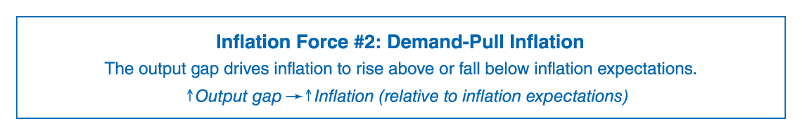
Excess demand leads inflation to rise above inflation expectations.

Should you raise prices?
A strong economy puts millions of businesses in a similar situation to Outback Steakhouse, with customer demand exceeding what producers can supply. Each of these businesses will respond to their excess demand much as Outback did, by raising their prices by a bit more than required just to keep pace with expected inflation. The result is demand-pull inflation, which occurs when excess demand pulls inflation up, so that it rises above expected inflation.
Insufficient demand leads inflation to fall below inflation expectations.
Demand-pull inflation can also pull inflation below inflation expectations when demand is unexpectedly weak. To see why, let’s return to the dark days following the financial crisis, when the economy was so weak that few people had extra cash to spend on restaurant meals. Outback’s 2009 annual report noted that “depressed economic conditions in 2009 and 2008 have created a challenging environment for us and … we experienced declining revenues, comparable store sales and operating cash flows and incurred operating losses each year.” These losses reflect the reality that half-empty restaurants are rarely profitable.

How can you bring in the crowds?
Outback was facing a problem of insufficient demand, as the quantity of restaurant meals demanded at the prevailing price was far below the quantity that Outback wished to supply. In response, Outback cut its prices. CEO Jeff Smith rolled out a new menu whose main feature was “prices that are easy on the wallet,” including 15 meals under $15, and some as low as $9.95. He says that decision was one of his most difficult moments as a manager, but ultimately one of his most important successes. These lower prices helped Outback return to profitability. It was profitable because the marginal cost of serving extra meals was particularly low as Outback’s staff barely had enough customers to stay busy.
In a weak economy, millions of businesses face insufficient demand. Like Outback, most will find that their marginal costs are low when they’re producing well below their capacity. They’ll follow the same logic as Jeff Smith and respond to insufficient demand with price restraint, either raising their prices by a bit less than they otherwise would or in some cases cutting them. Across the whole economy, the result is widespread price restraint that pulls inflation below expected inflation. That is, insufficient demand leads inflation to fall below expected inflation.
When the economy is operating at full capacity, inflation equals inflation expectations.
Notice that demand-pull inflation is a separate force that operates in addition to inflation expectations. When there’s excess demand, it pulls inflation to rise above inflation expectations, and when there’s insufficient demand, it pulls inflation to fall below inflation expectations.
Between these two cases—of excess demand and insufficient demand—is the case where demand matches the economy’s productive capacity. In this case there’s no demand-pull inflation and hence no pressure for prices to rise faster or slower than expected. And so when the economy is operating at full capacity, inflation is equal to inflation expectations.
The output gap measures the imbalance between output and productive capacity.
In all of this, the driver of demand-pull inflation is the imbalance between buyers’ demand for output versus the productive capacity of suppliers. This suggests that demand-pull inflation is driven by the output gap, which measures actual output relative to potential output.
The Phillips Curve Framework
Putting these pieces together yields two key observations that form the basis of the framework we’re building to analyze inflation.
Observation one: Demand-pull inflation is driven by the output gap.
When output exceeds potential output—meaning the output gap is positive—there is excess demand. The more positive the output gap is, the greater the degree of excess demand, and hence the greater the pressure to raise prices. By contrast, when output falls short of potential output—meaning the output gap is negative—there is insufficient demand. The more negative the output gap is, the greater the degree of insufficient demand, and hence the greater the pressure for price restraint.
Observation two: Demand-pull inflation leads inflation to diverge from inflation expectations.
Demand-pull inflation occurs in addition to inflation expectations, meaning that demand-pull factors cause inflation to either rise above inflation expectations (when there’s excess demand), or fall below inflation expectations (when there’s insufficient demand). That is, it drives unexpected inflation, which is the difference between inflation and inflation expectations:

The Phillips curve describes how the output gap is linked to unexpected inflation.
Put these two observations together, and we conclude that the output gap causes inflation to rise above, or fall below, inflation expectations. We can summarize this as follows:
Demand-pull inflation creates a link between the output gap and unexpected inflation (the gap between inflation and inflation expectations). When you graph this link, the result is known as the Phillips curve. Figure 6 shows the Phillips curve, illustrating how the output gap affects unexpected inflation.
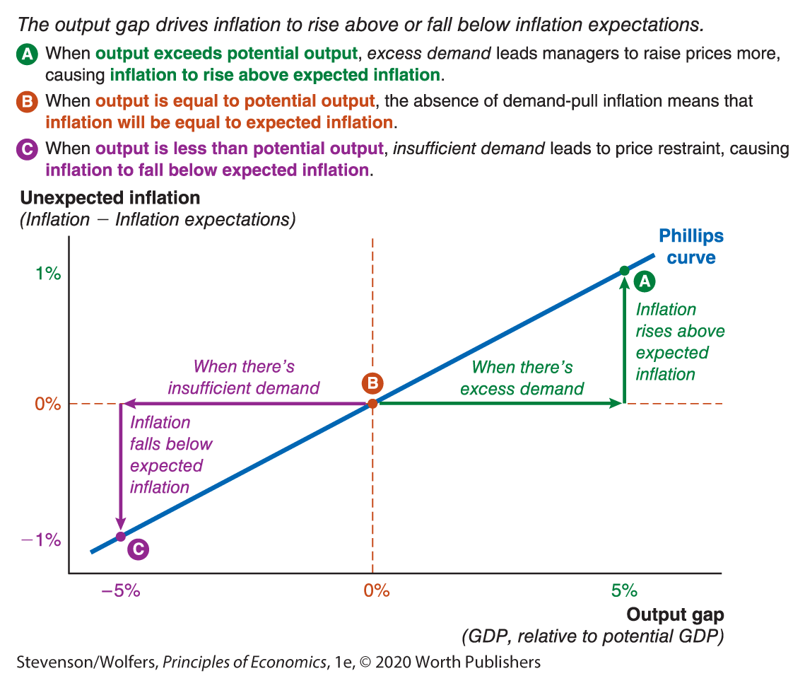
Figure 6 | The Phillips Curve
The Phillips curve is named after Bill Phillips who first discovered it. He was a bit of a character—a crocodile hunter, adventurer, and war hero, who once jerry-rigged a secret miniature radio while captured in a prisoner-of-war camp. While he only passed his economic principles class by a single point, he went on to make a major mark on the field by showing that excess demand generates inflationary pressure. His analysis of historical data unearthed the importance of demand-pull inflation.
Let’s explore this graph in a bit more detail.
Unexpected inflation goes on the vertical axis, and the output gap goes on the horizontal axis.
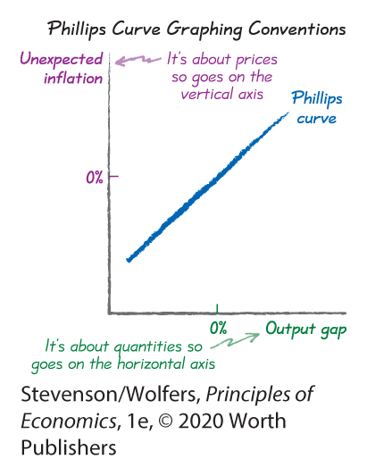
By now, you’re pretty familiar with the graphing convention in economics of using the horizontal axis to show what’s going on with quantities and the vertical axis to show what’s going on with prices. The same conventions apply to the Phillips curve, so make sure you put the output gap (which is about quantities) on the horizontal axis, and unexpected inflation (which is about prices!) on the vertical axis. And don’t forget that the Phillips curve describes inflation above and beyond that caused by inflation expectations, which is why the vertical axis measures unexpected inflation (which is inflation less inflation expectations).
One more graphing tip: Both the output gap and unexpected inflation can be either positive or negative, so it’s usually a good idea to extend both axes into negative territory. That means you draw the axes so that zero is pretty much in the middle. (This may seem unusual at first—it means the axes no longer rise from zero—but you’ll see that the curve still makes sense when you draw it.)
The Phillips curve is upward-sloping.

The Phillips curve is upward-sloping because higher output relative to potential output—a more positive output gap—leads to greater inflationary pressure, causing inflation to rise above inflation expectations. It illustrates the idea that:

When output is equal to potential output, then inflation is equal to expected inflation.
The Phillips curve passes through the origin, which is the point at which the output gap is zero and unexpected inflation is zero. At this point, output is equal to potential output and so the absence of demand-pull inflation means that inflation is pulled neither above nor below inflation expectations. As a result, when actual output is equal to potential output, actual inflation is equal to expected inflation.
The Phillips curve predicts how far inflation will diverge from expected inflation.

Notice that the vertical axis of the Phillips curve suggests that unexpected inflation can be either positive or negative. This doesn’t mean that actual inflation is likely to be negative (that can also happen, but it’s rare). Rather, the Phillips curve is all about unexpected inflation. When it says that unexpected inflation will be negative, this simply means that actual inflation will be less than expected inflation. And positive rates of unexpected inflation tell you that actual inflation will be greater than expected inflation. Indeed, the Phillips curve is useful because it tells you by how much actual inflation will be above or below expected inflation.
EVERYDAY Economics
How Uber is like the Phillips curve
As the concert ends late on a rainy Saturday night, you head outside, pull out your phone, and tap on the Uber app, hoping to summon a ride home. But the app responds that a ride that would normally cost $10 will now cost $30. You look around at the hundreds of other concert goers nearby, and your inner Bill Phillips explains what’s just happened: There are more concert-goers trying to get a ride home than available Uber drivers, so there’s excess demand.

It’s like the Phillips curve.
Uber’s surge-pricing algorithm has kicked in. It’s like a turbo-charged Phillips curve, programmed to respond to excess demand by raising prices immediately. We say it’s turbo-charged because it usually takes other businesses months rather than minutes to change their prices in response to a surge in demand. That’s why the Phillips curve typically describes inflation rising or falling over a period of months.
There’s one important difference. During that brief post-concert surge, most other prices—the price of taxis, of buses, or even of rental cars—are unchanged. As such, Uber’s surge pricing is best viewed as a change in relative prices—it raises the price of taking an Uber relative to taking the bus. By contrast, the Phillips curve describes how a surge in demand across the whole economy leads many businesses to raise their prices, and these widespread price rises create inflation.

The Phillips Curve in the United States
Bill Phillips once described his curve as a “wet weekend’s bit of work.” He discovered it by plotting historical data for the United Kingdom covering the period from 1861 through to 1957. It’s time for us to update his plots with an eye to discovering the modern Phillips curve for the United States.
Discover the Phillips curve for the United States.
We begin by compiling the relevant historical data. To construct our measure of unexpected inflation, we need to collect data on both the actual inflation rate each year and expected inflation (and here, I’m relying on the measure based on forecasts of professional economists). We calculate unexpected inflation simply as actual inflation less expected inflation. Next, we plot unexpected inflation in each year against the corresponding output gap.
Figure 7 plots these data, showing the shape of the Phillips curve for the United States. You’ll see that these data roughly bear out the predictions of our analysis: When the output gap is positive so that GDP is high relative to potential GDP, inflation has typically risen higher than inflation expectations. And when the output gap is negative so that GDP is low relative to potential GDP, inflation has typically fallen lower than inflation expectations. The upward slope of this curve reveals that the more positive the output gap, the more unexpected inflation there is.
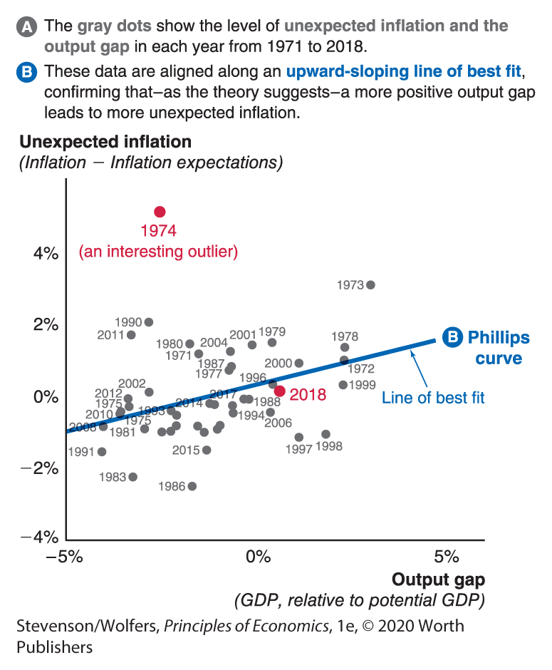
Figure 7 | Discover the Phillips Curve for the United States
Data from: Bureau of Economic Analysis; Bureau of Labor Statistics; Federal Reserve Bank of Philadelphia; Congressional Budget Office.
The data also reveal that this prediction isn’t always borne out, illustrating that the Phillips curve is an imprecise relationship. Even so, it remains an important tool because accounting for the output gap leads to more accurate inflation forecasts. The fact that the data do not lie exactly along this Phillips curve suggests that other factors also play a role. For example, the dot for 1974 (in the top left) is nowhere near the Phillips curve. That was a year in which oil prices unexpectedly rose sharply, and we’ll come back to explaining why that boosted inflation shortly.
When economists try to figure out what the Phillips curve looks like, they compile data like this and compute a line that best fits the data. The line of best fit in Figure 7 is an example of this sort of analysis. You could do this with a pencil, a ruler, and a bit of judgment, but in the example shown here, I’ve computed the line of best fit using a spreadsheet. (If you’ve taken a statistics class, you’ll recognize this as a regression line; if you haven’t, all you need to know is that this line best describes the relationship on average.)
A more complete analysis would also take account of other factors that might affect inflation, such as changes in oil prices, productivity, or the exchange rate. For now, be patient—we’ll incorporate these supply-side factors shortly.
Use the Phillips curve to forecast future inflation.
Investment banks, businesses, and government economists forecast inflation by using estimates of the Phillips curve that are similar to our line of best fit.
It’s a two-step process:
Step one: Assess inflation expectations. You can measure inflation expectations by analyzing surveys of inflation expectations, surveys of economists, or financial market-based measures.
Step two: Forecast unexpected inflation. This is where the Phillips curve is useful. Start with your estimate of what the output gap will be, look up to the corresponding point on the Phillips curve, and then look across to find your forecast for unexpected inflation. For instance, Figure 8 shows that an output gap of +5% corresponds with unexpected inflation of 1%.
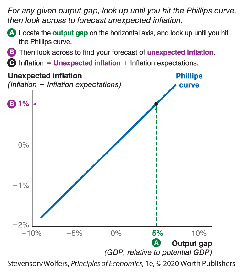
Figure 8 | Use the Phillips Curve to Forecast Inflation
Your inflation forecast, of course, should be the sum of your forecasts for expected inflation and unexpected inflation. So if inflation expectations are running at 2% and you’re also forecasting demand-pull inflation to add another 1%, you should forecast inflation to be 3%.
Do the Economics
You’re about to negotiate your salary for next year, and want to make sure that it adjusts for likely changes in the cost of living. The economy is doing well, and you expect GDP to be 5% above potential output. Inflation expectations are currently 2%.
- Using the Phillips curve in Figure 8, how much of a pay raise will you need to request to be able to buy the same stuff you currently buy?
- What if GDP is 2.5% below potential instead?
- What if GDP is exactly equal to potential GDP?

An Alternative Illustration: The Labor Market Phillips Curve
So far, we’ve described the Phillips curve as the relationship between unexpected inflation and the output gap. We focused on the output gap because it’s a measure of output relative to the economy’s productive capacity, and so it describes the extent to which managers are dealing with excess demand (which leads them to raise their prices a bit more) or insufficient demand (which leads them to show price restraint). The Federal Reserve has used the output gap and the Phillips curve to forecast inflation since at least the mid-1980s.
But historically the Phillips curve was drawn a little differently—partly because Phillips’ insights pre-dated modern methods to measure the output gap. This alternative version represents the same ideas, it was just sketched a little differently. Some economists even prefer this alternative version, so it’s worth becoming familiar with it.
The labor market Phillips curve links unexpected inflation to the unemployment rate.
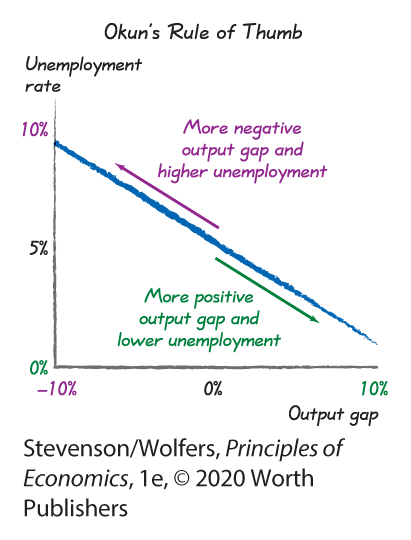
This alternative approach focused on the labor market. It noted that unemployed workers are an unused resource, and so the unemployment rate—which is the share of the labor force without a job—provides an alternative measure of whether the economy is producing above or below its productive capacity. Indeed, in Chapter 29, we saw that Okun’s rule of thumb describes a close link between the output gap and the unemployment rate. It says that a high unemployment rate corresponds with a negative output gap (where output is below potential output, and so insufficient demand is a problem). It also says that an especially low unemployment rate corresponds with a positive output gap (where output exceeds potential output, and so excess demand arises).
It follows that there’s an alternative version of the Phillips curve that links low unemployment to higher demand-pull inflation. We can summarize it as saying:

Both versions of the Phillips curve tell the same story.
This alternative version of the Phillips curve, which is illustrated in Figure 9, links inflation to unemployment. In order to keep the concepts clear, we’ll call this version the labor market Phillips curve. It summarizes the exact same ideas as the Phillips curve, but it relies on a different measure of excess demand. The most obvious difference—that the curves slope in different directions—is purely cosmetic. It arises only because excess demand corresponds with a high level of GDP relative to potential output, but a low unemployment rate. Both versions of the Phillips curve suggest that excess demand leads to higher inflation.

Figure 9 | The Labor Market Phillips Curve
Inflation is stable at the equilibrium unemployment rate.
The inflation rate will only be stable when inflation is equal to inflation expectations, and this occurs at the point where unexpected inflation is 0%. The corresponding unemployment rate is called the equilibrium unemployment rate. (You may also hear it called the “natural rate” or the NAIRU, which stands for the “non-accelerating inflation rate of unemployment”—a bit of a mouthful that’s trying to say it’s the only unemployment rate that will neither nudge inflation higher nor lower.) This is the only unemployment rate that’s consistent with stable inflation. The equilibrium unemployment rate is not zero because there remain potential workers who are facing frictional or structural barriers to unemployment. (Remember that we discussed why the equilibrium unemployment rate is not zero, in Chapter 23.) When unemployment is lower than the equilibrium unemployment rate, inflation starts to creep up. It’s hard to know with any precision what the equilibrium unemployment rate is—economists debate the matter endlessly—and so rather than emphasizing a particular number, it’s probably safer to say that it lies somewhere between 3% and 6%.
Demand-pull inflation is driven by too much demand.
We started this chapter by analyzing inflation expectations. We’ve now also analyzed the demand side of the economy, finding that excess demand creates demand-pull inflation, which causes inflation to rise above inflation expectations. (And insufficient demand causes inflation to fall below inflation expectations.)
While we’ve analyzed the role of demand in driving price changes, we’ve yet to explore the role of supply. Let’s fix that. As we turn to analyzing how changing supply conditions can produce inflation, we’ll discover that supply-side shocks shift the Phillips curve. But to see why, we’ll have to explore the link between Wonder Woman and geopolitics.