31.4 Supply Shocks Shift the Phillips Curve

Learning Objective Assess how shocks to production costs shift the Phillips curve.

A victim of geopolitical tension.

In 1974, a six-year old girl went to the toy store to buy a Wonder Woman action figure. She thought she had saved up enough to buy it, but when she arrived, she discovered that the price had risen. So she returned home, determined to keep saving her allowance. Several months later, she returned with what she now hoped was enough money. But again, the price had risen. Wonder Woman remained elusive. The six-year old’s hopes were dashed by geopolitical tensions that were about to roil the global economy.

Action figures are made of plastic, and plastic is made largely from oil, and much of the world’s oil comes from the Arabian Peninsula. Many oil-producing Arab nations were angered that the United States had supported Israel in the Yom Kippur War, so they retaliated by halting the sale of oil to the United States. This geopolitical disruption led to macroeconomic disruption. It caused a dramatic decrease in the supply of oil to the United States, which led the price of oil to quadruple in just a matter of months.

Expensive oil constituted a sharp increase in costs for American toymakers, who responded to these higher marginal costs by raising their prices. Similarly, the oil price hike raised marginal costs for the millions of other American businesses that use oil as an input. In response, these businesses also raised their prices. Inflation shot up from 6% in the middle of 1973 to 12% in 1974.

How Supply Shocks Shift the Phillips Curve

This was an example of cost-push inflation, where an unexpected boost to production costs pushed sellers to raise their prices.

Rising production costs create an additional reason to raise prices, above and beyond existing inflation expectations and demand-pull pressures. This means that cost-push inflation leads to more inflation at any given level of the output gap, and for any given level of inflation expectations. As Figure 10 illustrates, cost-push inflation causes the Phillips curve to shift.

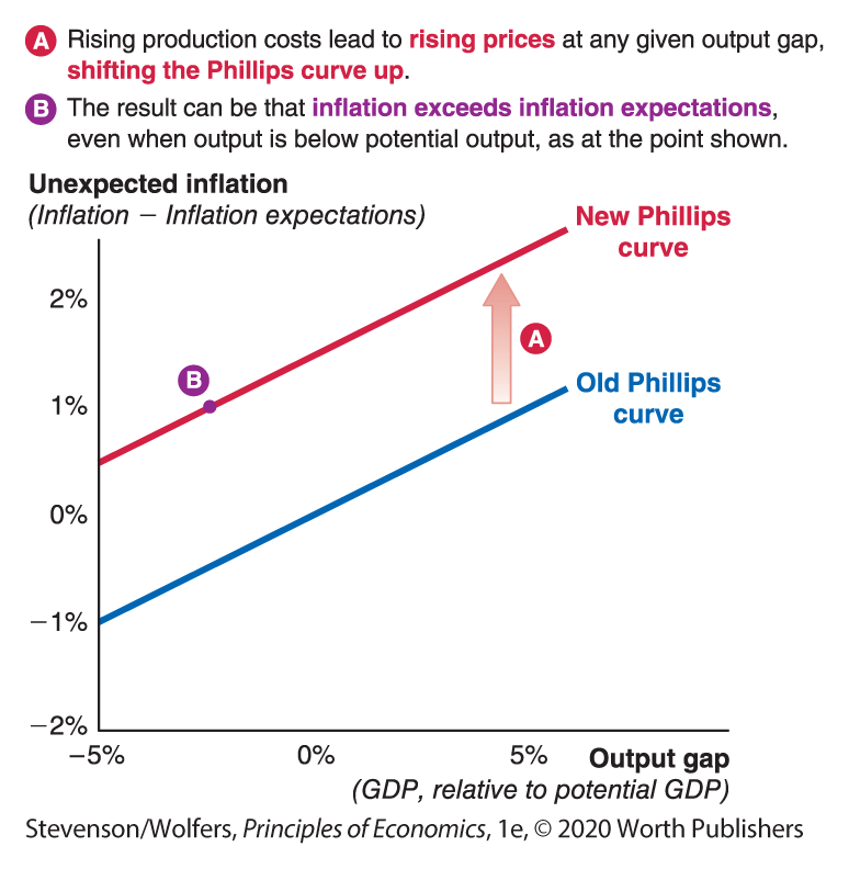
Figure 10 | Rising Costs Shift the Phillips Curve

The graph plots output gap (G D P relative to potential G D P) against unexpected inflation (inflation – inflation expectation) and shows two upward-sloping curves representing the old and new Phillips curves. The new Phillips Curve is above and parallel to the old Philip Curve. The text reads, A; Rising production costs lead to rising prices at any given output gap, shifting the Phillips curve up. B; The result can be that inflation exceeds inflation expectations, even when output is below potential output, as at the point shown.

Rising production costs shift the Phillips curve up.

Indeed, any factor that leads to an unexpected rise in production costs will cause the Phillips curve to shift upward. The reverse is also true: An unexpected decline in production costs will cause the Phillips curve to shift down as sellers respond by cutting prices (or raising them less).

This brings us to our third key insight about the causes of inflation:

Three types of supply shocks shift the Philips Curve.

This third inflationary force reflects the influence of unexpected changes in production costs, which is why it’s called cost-push inflation. And because changes in costs shift producers’ supply curves, an unexpected change in production costs that shifts the Phillips curve is called a supply shock.

supply shocks

Any change in production costs that leads suppliers to change the prices they charge at any given level of output. Supply shocks shift the Phillips curve.

The Phillips curve shifts in response to changes in:

1. Input prices
2. Productivity
3. Exchange rates

There are three key types of supply shocks that might shift the Phillips curve: shifts in input prices, shifts in productivity, and shifts in exchange rates. In each case we focus on an unexpected change in costs because anticipated rises or falls in input prices will have already been factored into inflation expectations. Let’s explore each in turn.

Phillips Curve Shifter One: Input Prices

The graph plots output gap against unexpected inflation and shows three upward-sloping curves. The curve in the middle depicts the Phillips curve, the curve above depicts the upward shift corresponding to rising input prices, and the third curve depicts the downward shift in the Phillips curve due to falling input prices.

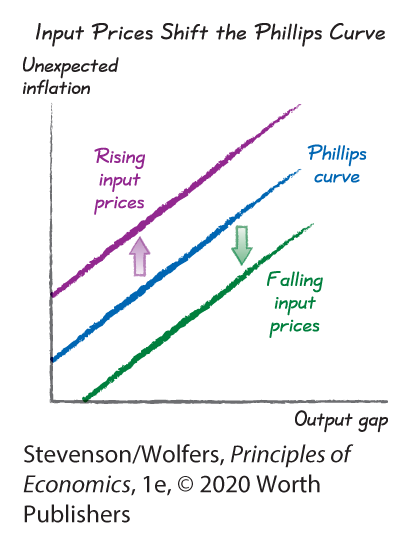
Any time the price of your inputs rises, so will your marginal costs, and higher marginal costs lead sellers to raise their prices. Thus, rising input prices lead to rising prices, and because this boosts inflation at any given level of the output gap, it shifts the Phillips curve up. The same forces also operate in reverse, and declining input prices shift the Phillips curve down. The more that an input price changes, and the more important that input is in the costs of a typical firm, the more it will shift the Phillips curve.

Oil and commodity prices are important input prices.

Oil is a major input in many sectors of the economy, and so the changing price of oil has frequently been an important source of cost-push inflation. Oil is important because it can be burned to generate electricity, refined into gasoline or diesel fuel, or synthesized into plastic (some of which might be used to make action figures). A rise in the price of oil has ripple effects throughout the economy, leading to higher electric and heating bills, higher gasoline prices, which lead to higher transportation prices, which raises the prices of nearly everything at your local supermarket. The oil price also bears watching because it has historically been so volatile, rising and falling in response to embargoes, wars, coups, and revolutions in the politically unstable Middle East, as well as unpredictable discoveries of new energy sources.

Other commodity prices—including agricultural goods in particular—can create supply shocks, particularly when severe weather disrupts harvests. It’s something that managers at Outback Steakhouse plan for, and indeed, its managers have said that “in most cases increased commodity prices could be passed through to our customers through increases in menu prices.” When other companies follow suit, commodity price shocks will generate widespread cost-push inflation.

Rising wages can cause a wage-price spiral.

The cyclic illustration shows that cost of production rises leading to a price rise leading to workers’ spending power falling leading to nominal wages rising in turn leading to a rise in cost of production.

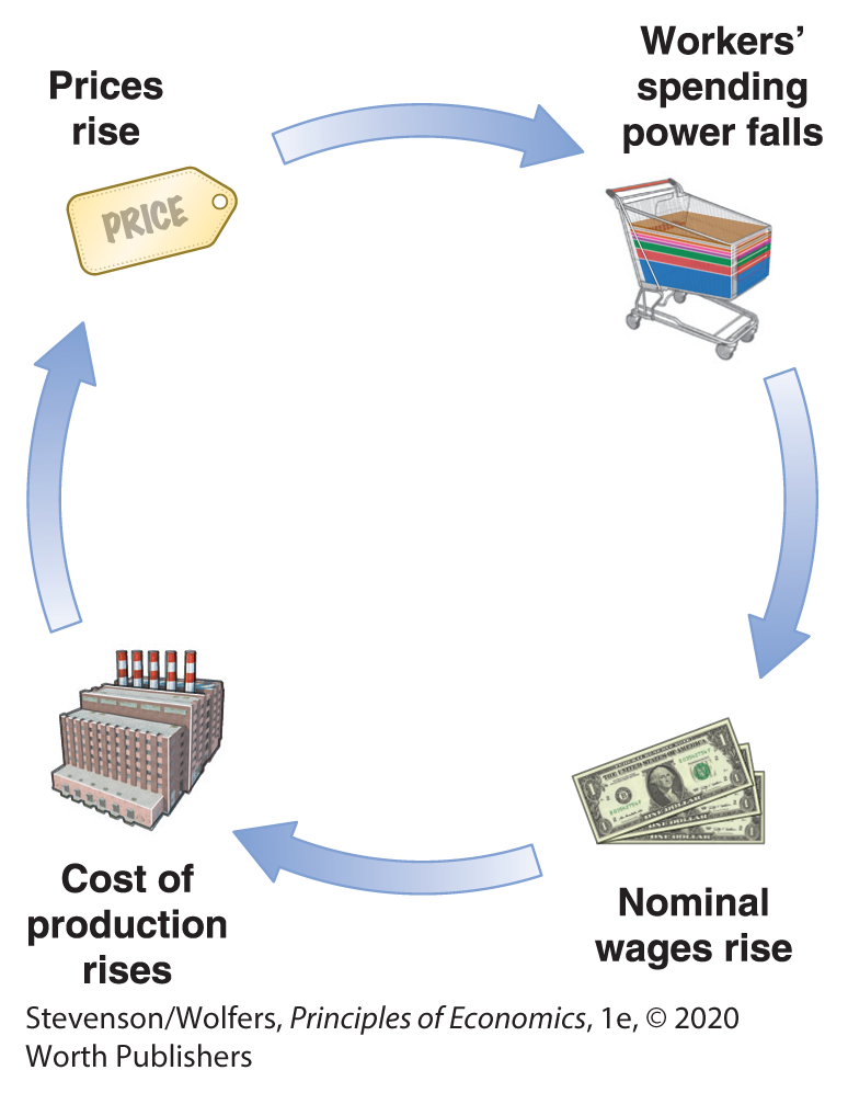
Perhaps the most important input price is the price of labor, otherwise known as the hourly wage. A sharp rise in the wages you have to pay to attract quality workers will raise your company’s marginal costs, causing many managers to raise their prices. Indeed, in the past, executives at Outback Steakhouse have reported that higher wages “have increased our labor costs … To the extent permitted by competition and the economy, we have mitigated increased costs by increasing menu prices.” Once again, as other companies follow suit, higher wages will quickly generate cost-push inflation.

Wages are particularly important because they can amplify the effects of a temporary inflation shock and make it persistent. This is because a wage-price spiral can take hold, in which workers respond to inflation by demanding higher nominal wages to maintain their spending power, leading businesses to respond to higher wages by raising prices. Thus, an initial inflationary impulse can cause workers to seek higher nominal wages, which causes businesses to further raise their prices, which causes workers to seek higher nominal wages, and so it continues as wages chase prices, and prices chase wages. The result is higher inflation that persists long after the initial inflationary impetus has receded.

wage-price spiral

A cycle where higher prices lead to higher nominal wages, which leads to higher prices.

Phillips Curve Shifter Two: Productivity

The graph plots output gap against unexpected inflation and shows three upward-sloping curves. The curve in the middle represents the Phillip curve, the curve above represents the upward shift due to slower productivity growth, and the curve below denotes the downward shift to faster productivity growth.

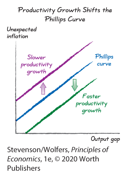
Your company’s productivity also changes your production costs, as a more productive firm needs less of each input to produce the same output. It follows that faster-than-expected productivity growth lowers your marginal costs, leading to greater price restraint at any given output gap. As a result, stronger productivity growth shifts the Phillips curve down—a form of negative cost-push inflation.

It also works the other way. Productivity growth through the 1960s had been quite rapid, and many businesses had gotten in the habit of giving their employees large nominal wage raises without it causing their per-unit costs to rise. But in the mid-1970s, productivity growth slowed even as wages continued to grow rapidly. The result was rising production costs that led to cost-push inflation. And so weaker productivity growth shifted the Phillips curve up.

Phillips Curve Shifter Three: Exchange Rates

The nominal exchange rate also creates cost-push inflation, thereby shifting the Phillips curve. There’s both a direct effect on the price of goods made overseas and an indirect effect due to the changing prices of foreign goods putting pressure on the prices of domestically produced goods.

Direct effect: When the U.S. dollar depreciates, foreign goods are more expensive.

A reminder: The exchange rate is the price of a U.S. dollar. For instance, when the exchange rate is 120 Japanese yen per dollar, that means that one U.S. dollar costs 120 Japanese yen. We say that the U.S. dollar depreciates when the price of a U.S. dollar falls, say to 100 yen. It means the U.S. dollar becomes cheaper for foreigners to buy; it also means that foreign currency is expensive for Americans to buy because it’ll cost more dollars to buy a specific quantity of yen.

This is relevant because you’ll need foreign currency to buy goods from foreigners. When the U.S. dollar depreciates, then each U.S. dollar buys less foreign currency. In turn, that means it’ll take more U.S. dollars to pay for imported goods. And so a depreciating U.S. dollar directly increases the price of foreign-made goods, boosting inflation.

Indirect effects: More expensive foreign goods lead to higher prices on domestic goods.

The graph plots output gap against unexpected inflation and shows three upward-sloping curves parallel to each other. The curve in the middle represents the Phillips curve, the curve with the upward shift corresponds to a depreciating U.S. dollar, and the curve with the downward shift corresponds to an appreciating U.S. dollar.

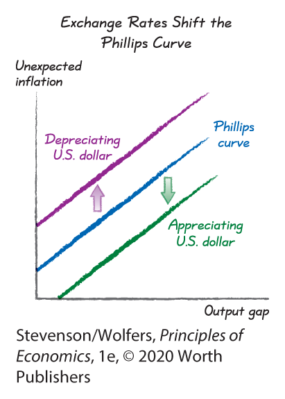
There are also indirect effects that lead American producers to raise their prices:

• For businesses that rely on imported inputs: A depreciating U.S. dollar raises the cost (in dollars) of their imported inputs, and these higher marginal costs lead them to raise their prices.
• For businesses that compete with imported products: A depreciating U.S. dollar raises the price (in dollars) of goods made by foreign competitors. This weakens the competitive pressure on domestic businesses, leading some of them to raise their prices.
• For businesses that export their products: A depreciating U.S. dollar means that their foreign customers are now willing to pay more (in dollars) for their products. This increased pressure from foreign customers may lead some companies to raise the prices they charge their American customers.

A depreciating U.S. dollar shifts the Phillips curve up; an appreciating U.S. dollar shifts the Phillips curve down.

Together, these direct and indirect effects mean that a depreciating U.S. dollar boosts inflation at any level of the output gap, thereby shifting the Phillips curve up. When the same forces operate in reverse, a rising value of the U.S. dollar—which we call an appreciation of the exchange rate—lowers inflation at any given output gap, shifting the Phillips curve down.

Shifts versus Movements Along the Phillips Curve

We’ve covered a lot of ground, so before we conclude, let’s recap. We’ll do so in a way that clarifies the difference between factors that cause a movement along the Phillips curve, and factors that cause a shift in the Phillips curve.

Demand-pull inflation leads to movement along the Phillips curve.

The Phillips curve illustrates the impact of demand-pull factors, showing how inflation changes in response to the output gap. Thus, booms and busts—which lead to changes in the output gap—represent movements along the Phillips curve.

A high output gap (increase in G D P relative to potential) leads to excess demand which leads to rising prices which leads to movement along the Phillips curve (upward and to the right). The accompanying graph plots output gap against unexpected inflation and shows an upward-sloping curve with arrows depicting upward movement along the slope from one point to another.

A low output gap (decreased G D P relative to potential) leads to insufficient demand which leads to falling prices (or slower rates of increases) which leads to movement along the Phillips curve (downward and to the left). The accompanying graph plots output gap against unexpected inflation and shows a downward-sloping curve with arrows depicting downward movement along the slope from one point to another.

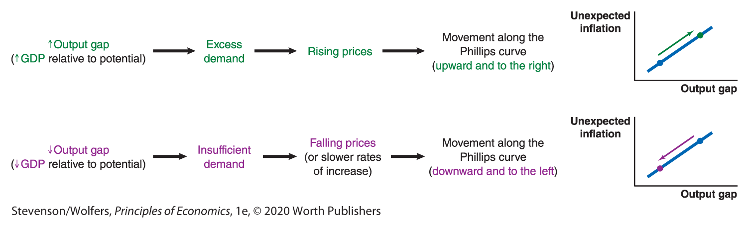
Cost-push inflation leads to a shift in the Phillips curve.

In contrast, any other factor that changes producers’ pricing decisions for a given output gap leads to a shift in the Phillips curve. A shift in your production costs creates pressure to shift your prices, and this occurs whatever the output gap is. We call these shifts supply shocks.

Rising production costs lead to higher marginal costs, causing businesses to raise their prices. The result will be higher inflation at any level of the output gap. Thus, rising production costs shift the Phillips curve up. On the flip side, falling production costs lead businesses to raise their prices by a bit less, or even cut them. The result will be lower inflation at any level of the output gap. Thus, falling production costs shift the Phillips curve down.

High input costs (oil, wages); low productivity growth and U.S. dollar value lead to rising production costs leading to rising prices at each output gap leading to the Phillips curve shifting up. The accompanying graph plots output gap against unexpected inflation and shows two parallel upward-sloping curves. The new curve is above the old curve indicating an upward shift.

Low input costs (oil, wages); high productivity growth and U.S. dollar value leads to falling production costs leading to falling prices at each output gap (or slower rates of increase) leading to the Phillips curve shifting down. The accompanying graph plots output gap against unexpected inflation and shows two parallel upward-sloping curves. The old curve is above the new curve indicating a downward shift.

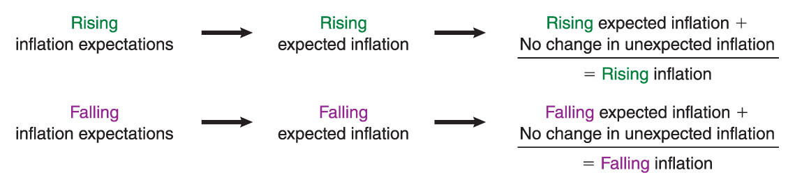
The Phillips curve is about short-run trade-offs, while inflation expectations remain relevant in the long run.

We began this chapter by describing inflation expectations as the key long-run cause of inflation. Inflation expectations neither shift the Phillips curve nor cause a movement along it, but they still play an important role in driving inflation. Recall that total inflation is the sum of expected inflation and unexpected inflation. The Phillips curve focuses on the short run in which inflation deviates from inflation expectations, and so it explains unexpected inflation. By contrast, rising inflation expectations lead to a rise in expected inflation. Thus, changes in inflation expectations are an important long-run factor determining overall inflation at any given level of the output gap and for any given constellation of input costs.

Rising inflation expectations lead to rising expected inflation in turn leading to rising expected inflation plus no change in unexpected inflation which equals rising inflation.

Falling inflations expectations lead to falling expected inflation leading to falling expected inflation plus no change in unexpected inflation which equals falling inflation.

Is it a demand shock or a supply shock?

You can use this framework to diagnose what’s going on in the economy. To see how, notice that demand-pull inflation always leads the output gap and unexpected inflation to move in the same direction: More output leads to higher inflation (for a given level of inflation expectations), while less output leads to less inflation (again, for a given level of inflation expectations). In contrast, supply shocks can lead to higher inflation, even when output has declined. This means that if you see the double-whammy of higher unexpected inflation and lower output, you can infer that there has been a supply shock. And if inflation rises in line with measures of inflation expectations, then you can infer that it’s inflation expectations that have shifted.