33.1 The AD-AS Framework

Learning Objective Understand how aggregate demand and aggregate supply determine macroeconomic equilibrium.

As you think about whether it’s a good time to buy a car; get ahead repaying your student loans; look for a new job; or pursue a graduate degree, your answers will likely depend—at least to some extent—on where you think the economy is going. That’s why our task in this chapter is to develop a framework that you can use to forecast where the economy is headed.

Introducing Aggregate Demand and Aggregate Supply

Much of this framework will feel familiar from your earlier analysis of how the microeconomic forces of demand and supply determine outcomes in individual markets, like the market for gasoline, coffee, or haircuts. We’re going to supersize these concepts and introduce you to their macroeconomic cousins, aggregate demand and aggregate supply, which describe the forces that determine aggregate outcomes such as total output and average prices across the economy as a whole.

Use the AD-AS framework to forecast output and the average price level.

This supersized version is called the AD-AS framework (that’s short for Aggregate Demand and Aggregate Supply), and it focuses on two key macroeconomic outcomes:

• The quantity of output produced across the economy as a whole, which is measured by real GDP; and
• The price of that output, which is measured by the GDP deflator. Think of this as the price of a basket containing the many goods and services we produce.

The graph plots quantity of output (real G D P) against price level (G D P deflator). Arrows with accompanying text read, Price goes on the vertical axis, Quantity goes on the horizontal axis; P’s before Q’s.

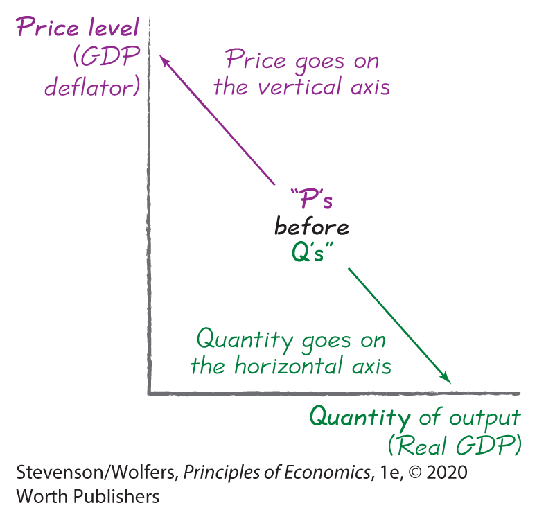
We’ll follow the usual convention in economics of plotting price on the vertical axis and quantity on the horizontal axis. Even if this seems familiar, there’s an important difference: This supersized framework isn’t about explaining the price and quantity of any individual good, but rather what’s happening to total output and average prices across the economy as a whole.

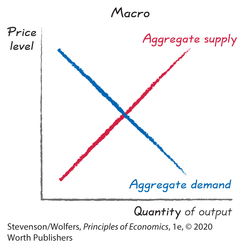
The aggregate demand curve is downward-sloping.

The aggregate demand curve (or “AD curve” to its friends) summarizes the purchasing plans of all buyers throughout the economy. It shows the relationship between the average price level and the total quantity of output that all buyers—consumers, businesses, the government, and overseas customers—collectively plan to purchase. A lower average price level leads buyers to demand a larger quantity of output, which means that the aggregate demand curve is downward-sloping.

aggregate demand curve

Shows the relationship between the price level and the total quantity of output that buyers collectively plan to purchase.

The aggregate supply curve is upward-sloping.

The aggregate supply curve (or “AS curve”) summarizes the production plans of all suppliers throughout the economy. It shows the relationship between the average price level and the quantity of output that suppliers collectively produce. A higher price level leads suppliers to produce a larger quantity of output, which means that the aggregate supply curve is upward-sloping.

aggregate supply curve

Shows the relationship between the price level and the total quantity of output that suppliers collectively produce.

Macroeconomic equilibrium occurs where the curves cross.

Scientists describe an equilibrium as a stable situation, with no tendency to change because opposing forces are in balance. This idea also applies to the economy as a whole: A macroeconomic equilibrium occurs when the quantity of output that buyers collectively want to purchase is equal to the quantity of output that suppliers collectively produce. As Figure 1 shows, macroeconomic equilibrium occurs at the point where the two curves cross.

macroeconomic equilibrium

Occurs when the quantity of output that buyers collectively want to purchase is equal to the quantity of output that suppliers collectively produce.

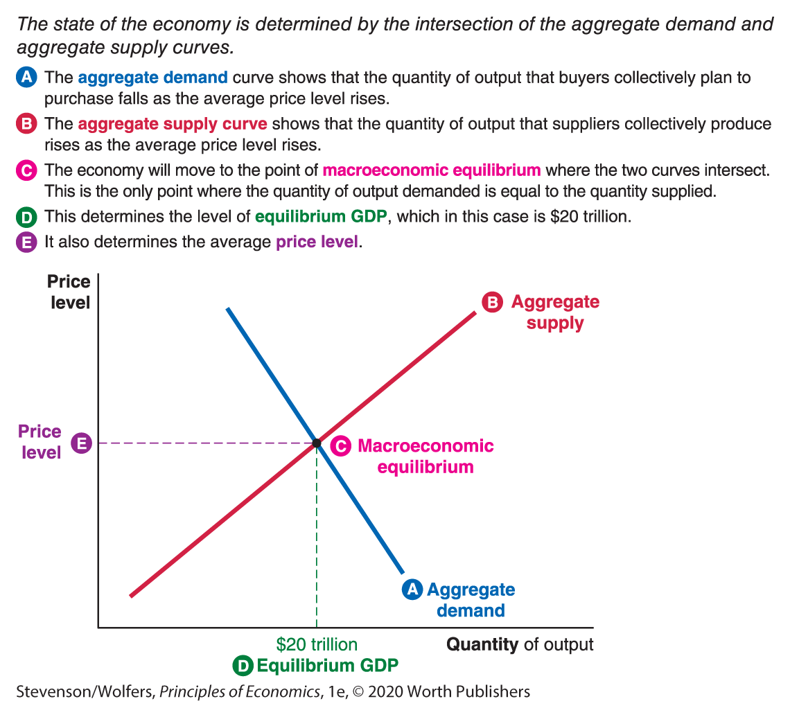
Figure 1 | The AD-AS Framework

The graph plots quantity of output against price level. The upward-sloping aggregate supply curve intersects the aggregate demand curve A at C, macroeconomic equilibrium. Dashed lines extend from the point E on the vertical axis and from point D on the horizontal axis to the point C

The text reads as follows:

The state of the economy is determined by the intersection of the aggregate demand and aggregate supply curves.

A, The aggregate demand curve shows that the quantity of output that buyers collectively plan to purchase falls as the average price level rises.

B, The aggregate supply curve shows that the quantity of output that suppliers collectively produce rises as the average price level rises.

C, The economy will move to the point of macroeconomic equilibrium where the two curves intersect. This is the only point where the quantity of output demanded is equal to the quantity supplied.

D, This determines the level of equilibrium GDP, which in this case is $20 trillion.

E, It also determines the average price level.

That’s it! You now have a powerful framework for forecasting both the level of GDP and the average price level in the economy. As we’ll discover, this framework is particularly useful for analyzing the year-to-year fluctuations that make up the business cycle.

Macroeconomic versus Microeconomic Forces

All that remains is to dig deeper into understanding the macroeconomic forces that underlie the aggregate demand and aggregate supply curves and to figure out when changing market conditions lead them to shift. That’s pretty much our whole agenda for the rest of this chapter.

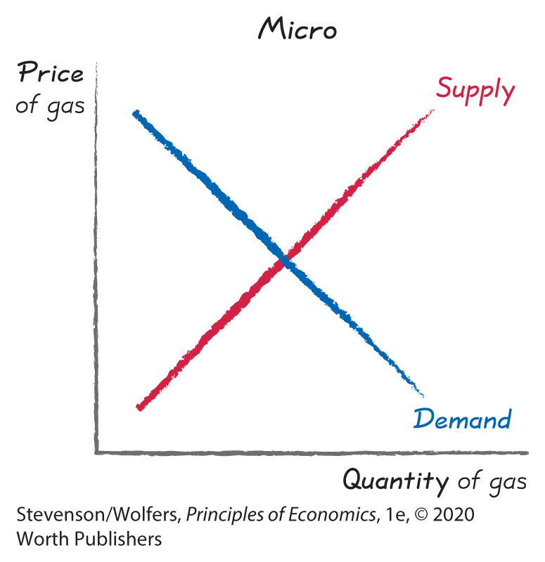
The AD-AS framework looks a lot like the microeconomic supply-equals-demand framework.

This approach should feel familiar from the microeconomic demand-equals-supply framework that we use to analyze individual markets. It’s familiar because in micro, as in macro, equilibrium occurs where the curves cross. And when market conditions change, you’ll forecast what will happen next by shifting the curves and finding the new equilibrium.

The graph plots quantity of gas against price level and depicts a downward-sloping demand curve and an upward-sloping supply curve that intersect each other.

But the AD-AS framework summarizes a different set of macroeconomic forces.

These different curves summarize different trade-offs. In a microeconomic context, the key opportunity cost of buying gasoline is not buying something else. But in a macroeconomic context we’re focused on spending on all goods and services, and so the relevant opportunity cost of buying output today is that you can’t save your money so that you can buy more output in the future. In micro, the key trade-offs are across products, while in macro the key trade-offs are across time.

Because the forces that shape these macroeconomic trade-offs are so different, it’s important that you label the curves in Figure 1 “aggregate demand” (or simply “AD”) and “aggregate supply” (or “AS”) rather than just “demand” or “supply.” The modifier “aggregate” is there to remind you to think about aggregate or macroeconomic forces. What are those forces? Glad you asked. That’s what we’re going to analyze next.

The graph plots quantity of gas against price level and depicts a downward-sloping aggregate demand curve and an upward-sloping aggregate supply curve that intersect each other.