33.2 Aggregate Demand
The aggregate demand curve summarizes the purchasing plans of all buyers throughout the economy at each possible price level. That means it describes the effect that the average price level has on the demand for output. To understand why the aggregate demand curve is downward-sloping, we need to dig into the forces that shape the total demand for output in the economy.
Aggregate Expenditure
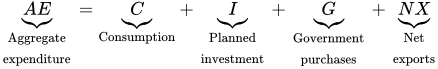
Aggregate expenditure refers to the total amount of goods and services that people want to buy across the whole economy—the sum of consumption, planned investment, government purchases, and net exports.
Aggregate expenditure is the sum of four components:
- = Consumption: When households buy goods and services
- + Planned investment: When businesses purchase new capital
- + Government purchases: When the government buys goods and services
- + Net exports: Spending by foreigners on American-made exports, less spending by Americans on foreign-made imports.
Economists often use abbreviations to simplify things, and so you might find it easier to write it this way:
When you’re trying to assess economy-wide demand, you need to focus on how much people (including businesses) want to buy, not the unsold inventories that companies accumulate. That’s why the measure of investment that’s counted in aggregate expenditure is planned investment, which includes all the spending on new capital by businesses but excludes unplanned changes in inventories.
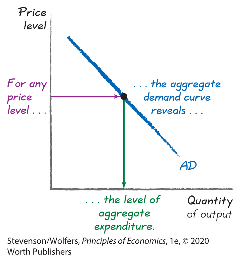
The aggregate demand curve illustrates the level of aggregate expenditure associated with different values of the aggregate price level. To see why this curve is downward-sloping, we’ll need to visit Washington, DC, to sit in on one of the most economically consequential meetings on the planet.
Why Aggregate Demand Is Downward-Sloping
Eight times a year, policy makers meet at the Federal Reserve—or “the Fed”—in Washington, DC. Over two days of meetings, they pore over binders full of data about how the economy is doing, discuss trends they’re seeing in different parts of the economy, debate the implications, and think through a variety of scenarios. When the meeting ends, the Fed announces its new setting for the interest rate.
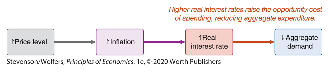
This is important because the real interest rate shapes aggregate expenditure and hence aggregate demand. Importantly, the Fed sets that interest rate based at least partly on what’s happening to the price level. As such, the Fed’s decisions are central to the relationship between the price level and aggregate expenditure illustrated by the aggregate demand curve. To see how, let’s step through each of the links in the chain connecting a higher price level to the quantity of output demanded.
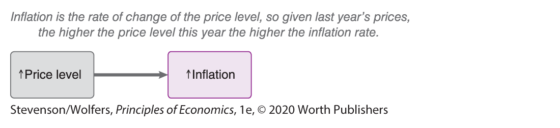
A higher price level corresponds to a higher inflation rate.

The larger the price rise, the higher this year’s inflation rate.
The first link follows from a definition: The inflation rate measures—in percentage terms—how much higher this year’s price level is than last year’s. Given that last year’s price level is set in stone, the higher this year’s price level is, the higher this year’s inflation rate will be.
Higher inflation leads the Fed to raise the real interest rate.
Here’s where the Fed comes in: The Federal Reserve tries to keep the inflation rate stable at its target level. When the inflation rate is either too high or too low, the Federal Reserve will adjust the real interest rate to bring inflation back toward its target level. Specifically, high inflation leads the Fed to raise the real interest rate, while low inflation leads it to lower the real interest rate. Thus, we have the next link in the chain connecting a higher price level to the quantity of output demanded:
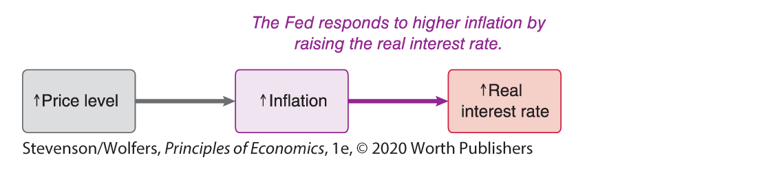
The process by which the Fed determines when to adjust interest rates, and how it goes about making those changes, is so important that we’ll devote all of Chapter 34, on monetary policy, to understanding how it does this. For now, it’s sufficient to note that the Fed responds to higher inflation by setting a higher real interest rate. A rough rule of thumb suggests that when the inflation rate is one percentage point higher, the Fed responds by setting the real interest rate half a percentage point higher.
A higher real interest rate leads to lower aggregate expenditure.
The opportunity cost of buying stuff today is earning interest and buying even more stuff in the future.
The real interest rate is the nominal interest rate adjusted for inflation, and it matters because it represents the opportunity cost of spending. The opportunity cost principle tells you that before spending money, you should ask, “Or what?” You can spend money now, or you can save it, earn interest, and buy even more in the future. The real interest rate tells you how much more stuff you’ll be able to buy if you wait until next year. A higher real interest rate corresponds to a higher opportunity cost of spending, and so it leads to less aggregate expenditure.
This is particularly true for investment because a higher real interest rate means that fewer investment projects will be profitable enough to offset the opportunity cost of keeping your money in the bank to earn interest. A higher real interest rate also reduces consumption partly because it raises the cost of borrowing to fund big-ticket items like a car. It can also cause net exports to decline through an exchange rate effect, in which inflows of foreign savings cause the U.S. dollar to appreciate, making American exports more expensive for foreigners. Together, these observations give us the final link in our chain connecting a higher price level to the quantity of output demanded—higher real interest rates reduce aggregate expenditure, and hence the aggregate demand for output:
The aggregate demand curve is downward-sloping because a higher price level leads to less aggregate demand.
Put the links together, and we’ve explained why the aggregate demand curve is downward-sloping: The higher this year’s average price level, the higher is the inflation rate; the Fed responds to inflation by raising the real interest rate; and this higher interest rate leads to lower levels of spending, and hence less aggregate demand:
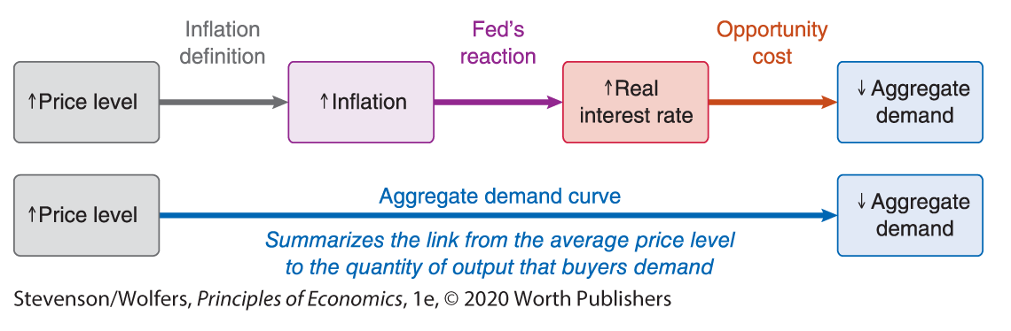
The aggregate demand curve summarizes this logic, showing that a higher price level ultimately leads buyers to demand a lower quantity of output. The same forces also operate in reverse, and so they also show that a lower price level leads buyers to demand a higher quantity of output. Because the Fed plays an important role in this process, this is sometimes called the Fed channel.
The Fed channel operated differently in the past.
Earlier economists had a somewhat different description of the Fed channel, describing it instead as an interest rate effect. This is because back in the 1970s the Fed didn’t set interest rates directly; instead it focused on hitting pre-announced targets for the nominal money supply, which is the quantity of money in circulation. If the price level rose, then the real money supply—that is, the quantity of money measured in terms of its purchasing power—would mechanically fall. A decrease in the real money supply has the effect of pushing the real interest rate up. The underlying insight of the interest rate effect—that a higher price level can lead to a higher real interest rate which reduces output—remains relevant. The only difference is that today the Fed sets the interest rate directly, rather than setting the nominal money supply and passively allowing the interest rate to respond. The Fed channel describes this more modern version of the interest rate effect in which the Fed directly raises the interest rate in response to inflationary price rises, which reduces output.
There are other economic forces that also lead the aggregate demand curve to be downward-sloping.
In addition to the Fed channel, there’s an international trade effect, in which a higher price level in the United States leads American-made products to become more expensive relative to foreign goods. Thus, a higher price level reduces net exports, and hence aggregate expenditure. Because net exports is a small component of aggregate expenditure, this effect tends to be small.
There’s also a wealth effect, in which a higher price level reduces real wealth by reducing the purchasing power of assets whose values are fixed in nominal dollars—like the cash in your wallet. Lower real wealth leads people to spend less. This effect is likely small for two reasons. The first is that, as you learned in Chapter 25 on consumption, changes in wealth tend to lead to relatively small changes in spending. The second is because there is an offsetting debt effect because a higher price level reduces the real value of people’s nominal debts, which leads them to spend more.
Analyzing Aggregate Demand
The aggregate demand curve is useful because you can use it to forecast the consequences of changing market conditions. As you do so, be sure to distinguish between the effects of a change in the price level—which will cause a movement along the aggregate demand curve—from shifts in other factors, which shift the curve.
Changes in the price level lead to movements along the aggregate demand curve.
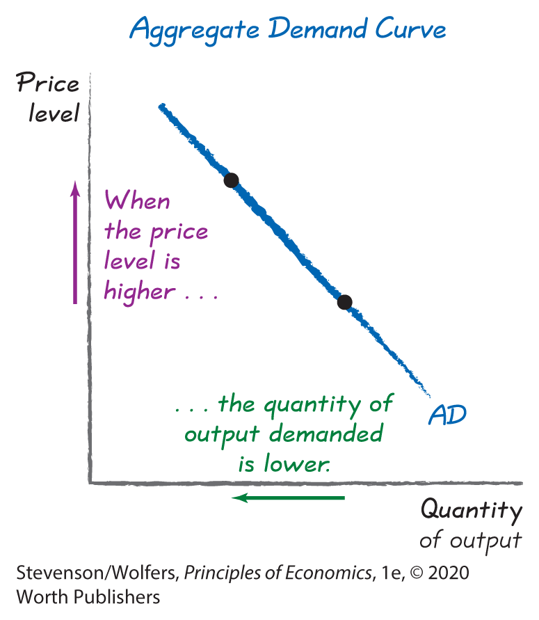
The aggregate demand curve illustrates how different price levels lead to differences in the quantity of output demanded. It’s useful because when the price level changes, you can simply consult this curve to figure out the new quantity of output demanded. The green arrow in Figure 2 illustrates how a higher price level leads to a movement along the aggregate demand curve to a new point that corresponds to a lower quantity of output demanded. The purple arrow shows that a lower price level leads to a movement along the aggregate demand curve, but this time to a point where there’s a higher quantity of output demanded.
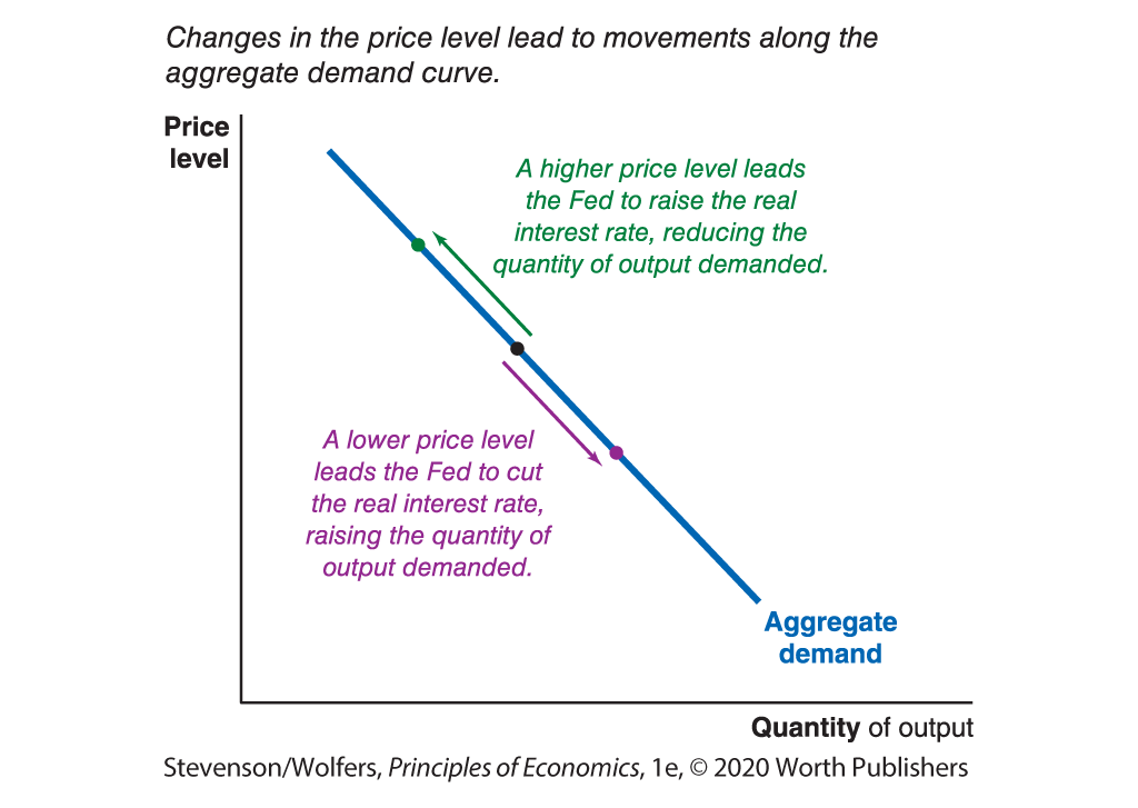
Figure 2 | The Aggregate Demand Curve
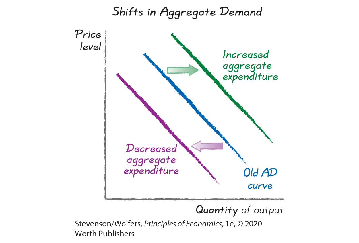
Changes in spending (at a given price level) shift the aggregate demand curve.
The aggregate demand curve shows the level of aggregate expenditure at each price level. Whenever consumers, investors, the government, or foreigners change their spending plans (at a given price level), the ensuing change in aggregate expenditure will cause the aggregate demand curve to shift.
A boost in spending that raises aggregate expenditure at a given price level causes an increase in aggregate demand, which shifts the aggregate demand curve to the right. The new equilibrium will occur where this new aggregate demand curve intersects the aggregate supply curve. As Panel A on the left of Figure 3 shows, an increase in aggregate demand leads the economy to move to a new equilibrium which results in a rise in GDP and a rise in the price level. That means that increasing aggregate demand leads to a period of rising GDP (which we call an expansion) and rising prices (which you should recognize as inflation).
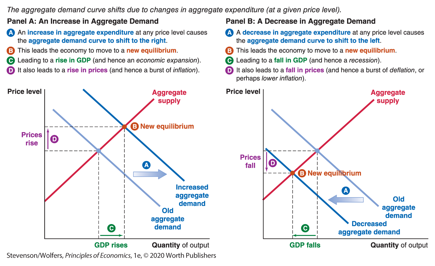
Figure 3 | Shifts in Aggregate Demand
By contrast, spending cuts that decrease aggregate expenditure at a given price level will cause a decrease in aggregate demand, shifting the aggregate demand curve to the left. As Panel B on the right of Figure 3 shows, a decrease in aggregate demand leads the economy to move to a new equilibrium which results in a fall in GDP and a fall in the price level. It follows that decreasing aggregate demand leads to a recession (a period of declining economic activity), and deflation (in which the price level is falling). In reality, many economies experience ongoing inflation for other reasons, and so a decrease in aggregate demand might lead to a decrease in inflation, rather than outright deflation.
Aggregate Demand Shifters
So far we’ve seen that shifts in aggregate demand have an important influence on business cycle conditions. Our next task is to identify the sorts of changes that might catalyze a shift in aggregate expenditure and hence the aggregate demand curve. Remember, 
Demand shifter one: Consumption increases when people feel more prosperous.

They’re shifting the aggregate demand curve.
People typically increase their spending when they have more money to spend, or are confident that they soon will. Thus, any development that makes people feel more prosperous—or more confident that they will soon be prosperous—leads to an increase in consumption, thereby increasing aggregate demand. This means that consumption will shift in response to:
Wealth: When the stock market booms or house prices rise, stockholders and homeowners feel more prosperous because their wealth has increased. As those lucky stockholders and homeowners spend some of their newfound wealth, consumption will increase.
Consumer confidence: The interdependence principle reminds you that the decisions you make today depend on your expectations about what’s going to happen in the future. And when you feel confident that your income will grow in the future, you might ramp up your spending in advance. As a result, consumption increases when an improved economic outlook boosts consumer confidence.
Taxes and government assistance: When the government cuts taxes, or when it increases government assistance payments like unemployment insurance, people have more disposable income that they can use to buy stuff. And so consumption increases when government policy puts more money in people’s pockets.
Inequality: People with low incomes tend to spend a larger share of their income than do those with higher incomes. It follows that redistributing income from those with higher incomes to those with lower incomes—including through government transfer payments and changes in the tax system—tends to increase consumption.
Demand shifter two: Investment increases when it’s profitable for businesses to expand.

It’s only a worthwhile investment if the opportunity cost isn’t too high.
As a manager, you’ll invest in new machinery when you believe that it will be profitable to expand your production. The cost-benefit principle reminds you to consider both the benefits of the extra revenue you’ll earn from enhancing your production capacity, and the cost of making that investment. As a result, aggregate demand will shift when investment changes in response to:
An expanding economy: When the economy is expanding, so is the demand for goods and services. In order to produce more, managers will need to expand their production capacity, and entrepreneurs will see an opportunity to start new businesses. As a result, investment in new equipment increases when the economy is expanding more rapidly.
Business confidence: Because capital investments tend to last for years, or even decades, your assessments about whether to buy new equipment should depend not only on today’s profits, but also on your expectations about future profitability. That’s why investment increases when managers are more confident about their future profitability.
Corporate taxes: Lower corporate taxes increase the after-tax profits that entrepreneurs earn from investing in new equipment. As a result, investment increases in response to a cut in corporate tax rates. Investment also increases in response to targeted investment tax credits that reduce the after-tax cost of buying new equipment.
Lending standards and cash reserves: If your business finds it hard to borrow money at a reasonable interest rate, your best alternative is to invest in new equipment only when your company has the cash on hand to do so. It follows that investment tends to increase when loans are easier to get, or businesses have large cash reserves. Cash reserves are particularly important when the financial system is not working well.
Uncertainty: If you’re uncertain about the economic outlook—it could be great, it could be terrible—remember that you usually have the option to postpone breaking ground on major investment projects until the outlook is a bit clearer. Lower uncertainty leads managers to restart these shelved projects, leading to an increase in investment.
Demand shifter three: Government purchases increase when policy makers decide to spend more on goods and services.
For example, they may pass legislation that increases government spending on highways or military equipment. In some cases, these spending bills have the explicit goal of stimulating an increase in aggregate demand. In addition, some government programs—known as automatic stabilizers—automatically increase spending when the economy is weak.
Remember that government spending only directly increases aggregate expenditure—and hence shifts the aggregate demand curve—when the government purchases goods and services. By contrast, many government programs—such as unemployment insurance or Social Security—simply transfer money from one bank account (the government’s) to another (the recipient’s), and so they don’t directly increase aggregate expenditure. There may however be an indirect effect, as redistributing money to people who are more likely to spend it might increase consumption.
Demand shifter four: Net exports increase due to global factors.
Global factors determine net exports.
Net exports rise when people in other countries want to buy a lot of American-made goods and services. It’s the interdependence principle at work, as net exports link the U.S. economy with economies around the world. Aggregate demand will shift when net exports rise or fall in response to:
Global economic growth: When the economies of Europe, Japan, and China do well, their consumers and businesses have more money to spend, and so they buy more goods, including more American-made goods, leading net exports to increase.
The exchange rate: Net exports also shift in response to changes in the exchange rate. When the U.S. dollar becomes cheaper, our goods become cheaper to foreign buyers, leading exports to rise. A cheaper U.S. dollar also means that foreign goods become more expensive (in dollars) for American buyers, leading imports to fall. Both forces—rising exports and falling imports—cause net exports to increase.
Trade barriers: Exports increase when there are fewer barriers preventing American businesses from selling their goods in other countries, while imports increase when there are fewer barriers preventing foreign businesses from selling to buyers in the United States. Because trade agreements typically reduce barriers to both imports and exports, their effect on net exports (which is exports less imports) is unclear. Likewise trade wars—in which higher trade barriers preventing imports lead other countries to retaliate by raising barriers that prevent foreigners from buying American exports—will reduce both imports and exports, yielding an unclear effect on net exports.
Recap: Anything that shifts any component of aggregate expenditure shifts the AD curve.
At this point, this list of changes that can shift the aggregate demand curve might seem a bit exhausting. I’ve put it all together for you in Figure 4. But you don’t need to memorize this whole list, because it’s all about just one idea: The aggregate demand curve shifts in response to an increase in any component of aggregate expenditure. That’s the easy way to remember this list: It’s just C, I, G, and NX.
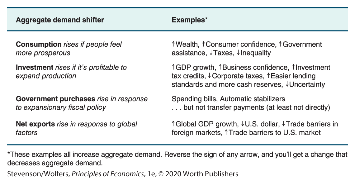
Figure 4 | Factors That Shift the Aggregate Demand Curve
There’s one more factor to consider—changes in the real interest rate. The interest rate matters because it can lead to changes in aggregate expenditure, particularly investment. But it won’t always lead the aggregate demand curve to shift. (Why? Remember that the aggregate demand curve already reflects the changes in aggregate expenditure due to the Fed adjusting interest rates in response to inflation.) We’ll dig into when and how changing interest rates shift aggregate demand in a few pages when we analyze monetary policy.
EVERYDAY Economics
How a recession is like a bad night’s sleep

You have nothing to fear, but fear itself.
It’s the night before a major exam, a big interview, or an important recital, and your mind races as you realize how important it is that you sleep well. Perhaps you’re lucky, and you fall asleep right away. But if you don’t, you might start to worry that you’re not yet asleep, which stresses you out … making it impossible to fall asleep. Essentially, your anxiety about not sleeping causes you not to sleep. I bet you know the feeling.
The thing is, if you can quiet your fear of not sleeping, you’ll find it easier to fall asleep. If you believe you can fall asleep, you probably will. It’s a self-fulfilling prophecy. The same kind of self-fulfilling prophecy that prevents you from getting to sleep can cause an economic boom or bust. If you fear that a recession’s looming, you might spend less. The problem is that if lots of people fear that a recession is looming, then lots of people will spend less, and aggregate demand will decrease. So if people fear a recession, there will probably be a recession. Pessimistic beliefs about the economy can create a pessimistic reality. President Franklin D. Roosevelt summarized this logic toward the end of the Great Depression, famously telling Americans that “the only thing we have to fear is fear itself.”
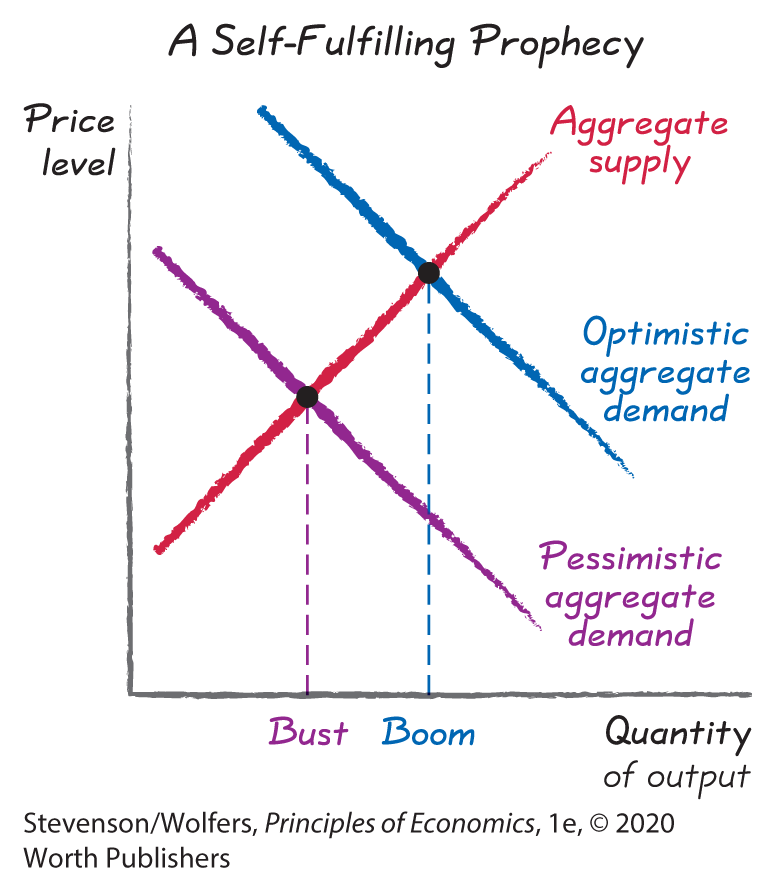
His speech was intended to help switch the economy from an equilibrium of self-fulfilling pessimism to one of self-fulfilling optimism. Roosevelt knew that if he could convince people that the economy would recover, then they would spend more. And if they spent more, the increase in aggregate demand would lead the economy to recover. A more optimistic expectation can also create a more optimistic reality. Remember FDR’s lesson next time you’re struggling to sleep: If you can quiet your fear of not sleeping, you’ll find it easier to fall asleep.
