Chapter 2

Continuous and linear maps

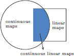
A normed space has two structures: a linear one (the underlying vector space), and a topological one (the norm). So when we study maps between normed spaces, it is natural to focus on maps which are well-behaved with these structures, and we’ll do this now. In particular, we’ll study:

(1)linear transformations
(well-behaved with respect to the linear structure),

(2)continuous maps
(well-behaved with respect to the topological structure),

(3)continuous linear transformations
(well-behaved with respect to both structures).

In the context of normed spaces, continuous linear transformations are most important, and these are sometimes also called bounded linear operators.

The reason for this terminology will become clear in Theorem 2.6 (page 67). We’ll see that the set of all bounded linear operators is itself a vector space, with obvious pointwise operations of addition and scalar multiplication, and it also has a natural notion of a norm, called the operator norm. Equipped with the operator norm, the vector space of bounded linear operators is a Banach space, provided that the co-domain is a Banach space. This is a useful result, which we will use in order to prove the existence of solutions to integral and differential equations.

2.1Linear transformations

Linear transformations are maps that respect vector space operations.

Definition 2.1. (Linear transformation).

Let X and Y be vector spaces over K (R or C).

A map T : X → Y is called a linear transformation if:

(L1) For all x₁, x₂ ∈ X, T(x₁ + x₂) = T(x₁) + T(x₂).

(L2) For all x ∈ X and all α ∈ K, T(α · x) = α · T(x).

Example 2.1. (Linear galore!)

(1)D : C¹[a, b] → C[a, b] given by Dx = x′, x ∈ C¹[a, b] is a linear transformation, since

(L1) D(x + y) = (x + y)′ = x′ + y′ = Dx + Dy for all x, y ∈ C¹[a, b];

(L2)D(αx) = (αx)′ = α · x′ for all α ∈ R and x ∈ C¹[a, b].

(2)Let m, n ∈ N and X = Rⁿ and Y = R^m.

is a linear transformation from Rⁿ to R^m. Indeed,

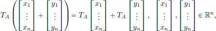
and so (L1) holds. Moreover,

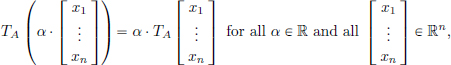
and so (L2) holds as well. Hence T_A is a linear transformation.

(3)Let X = Y = ℓ². Define the left/right shift operators L, R as follows: if x = (x_n)_n∈N ∈ ℓ², then

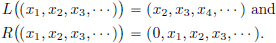
Then it is easy to see that R and L are linear transformations.

(4)Let X := c(⊂ ℓ^∞), the space of all real valued convergent sequences, and Y = R. The map L : c → R, L((a_n)_n∈N) := for (a_n)_n∈N, is a linear transformation (using the algebra of limits).

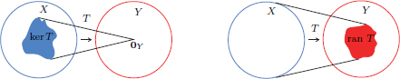
Recall that given a linear transformation T : X → Y, we can associate with T two natural subspaces, of X and Y, respectively,

the kernel of T, ker T := {x ∈ X : Tx = 0_Y} ⊂ X, and

the range of T, ran T := {y ∈ Y : ∃x ∈ X such that y = Tx} ⊂ Y .

In the above example of the linear transformation L, we have

ker L = c₀(set of sequences convergent with limit 0),

ran L = R(since for every r ∈ R, the constant sequence (r)_n∈N) converges to r).

(5)The map I : C[a, b] → R, given by for all x ∈ C[a, b], is a linear transformation.

(6)Let S := {h ∈ C¹[a, b] : h(a) = h(b) = 0}. From Exercise 1.3 (page 7), we see that S is a subspace of C¹[a, b]. Let A, B ∈ C[a, b] be fixed functions.

Let L : S → R be given by

Let us check that L is a linear transformation. We have:

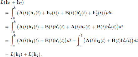
(L1) For all h₁, h₂ ∈ S,

(L2) For all h ∈ C¹[0, 1] and all α ∈ R,

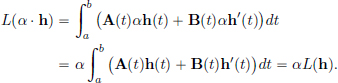
Thus L is a linear transformation.

(7)Let C¹(R), C²(R) denote the vector spaces of once, respectively twice continuously differentiable real-valued functions in R with pointwise operations. For f ∈ C²(R) and g ∈ C¹(R), consider the initial value problem for the one (spatial) dimensional wave equation:

Let C²(R × [0, ∞)) denote the vector space of all twice continuously differentiable functions (x, t) u(x, t) : R × [0, ∞] R, again with pointwise operations. Then it can be shown that the unique solution u_f,g in C²(R × [0, ∞)) to (IVP) is given by d’Alembert’s Formula,

Then the map (f, g) u_f,g : C²(R) × C¹(R) → C²(R × [0, ∞)) is a linear transformation.

Here are some non examples.

Example 2.2. (Not quite linear!)

(1)If ·^∗ denotes complex conjugation, then the complex conjugation map z z^∗ : C → C is not a linear transformation, since although (L1) is satisfied: (z + w)^∗ = z^∗ + w^∗(z, w ∈ C), we see that (L2) isn’t: indeed, (i · 1)^∗ = i^∗ = –i ≠ i · 1^∗.

(2)Consider the map T : R² → R² defined by

Then T is not a linear transformation since (L1) is not satisfied.

Indeed,

while

If α ∈ R\{0} and then we have

If α = 0 and

So for all Thus (L2) holds.

Notation 2.1. We will denote the set of all linear transformations from the vector space X to the vector space Y by L(X, Y). Recall from elementary linear algebra that L(X, Y) is itself a vector space (over the common field K for X, Y) with pointwise operations: if T, S ∈ L(X, Y), then we define T + S ∈ L(X, Y) by (T + S)(x) = Tx + Sx, for all x ∈ X, and if α ∈ K and T ∈ L(X, Y), then we define α · T ∈ L(X, Y) by (α · T)(x) = α · (Tx), for all x ∈ X. What is the zero vector in this vector space L(X, Y)? It is the “zero linear transformation” 0 : X → Y, given by 0x = 0_Y, for all x ∈ X, where 0_Y denotes the zero vector in Y.

If X = Y, then we write L(X) instead of L(X, X).

Exercise 2.1. Consider the two maps S₁, S₂ : C[0, 1] → R given by

Show that S₁ is not a linear transformation, while S₂ is.

Exercise 2.2. Let a, b be nonzero real numbers, and consider the two real-valued functions f₁, f₂ defined on R by f₁(t) = e^at cos(bt) and f₂(t) = e^at sin(bt), t ∈ R. f₁ and f₂ are vectors belonging to the infinite dimensional vector space C¹(R), consisting of all continuously differentiable functions from R to R. Denote by S_f1,f2 the span of the two functions f₁ and f₂.

(1)Prove that f₁ and f₂ are linearly independent in C¹(R).

(2)Show that the differentiation map, 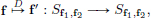is a linear transformation.

(3)What is the matrix [D]_B of D with respect to the (ordered) basis B = (f₁, f₂)?

(4)Prove that D is invertible, and write down the matrix corresponding to the inverse of D.

(5)Compute the indefinite integrals

2.2Continuous maps

Let X and Y be normed spaces. As there is a notion of distance between pairs of vectors in either space (provided by the norm of the difference of the pair of vectors in each respective space), one can talk about continuity of maps. Within the huge collection of all maps, the class of continuous maps form an important subset. Continuous maps play a prominent role in functional analysis since they possess some useful properties.

Before discussing the case of a function between normed spaces, let us first of all recall the notion of continuity of a function f : R → R.

Continuity of functions from R to R

In everyday speech, a ‘continuous’ process is one that proceeds without gaps of interruptions or sudden changes. What does it mean for a function f : R → R to be continuous? The common informal definition of this concept states that a function f is continuous if one can sketch its graph without lifting the pencil. In other words, the graph of f has no breaks in it. If a break does occur in the graph, then this break will occur at some point. Thus (based on this visual view of continuity), we first give the formal definition of the continuity of a function at a point below. Next, if a function is continuous at each point, then it will be called continuous. If a function has a break at a point, say x₀, then even if points x are close to x₀, the points f(x) do not get close to f(x₀).

This motivates the definition of continuity in calculus, which guarantees that if a function is continuous at a point x₀, then we can make f(x) as close as we like to f(x₀), by choosing x sufficiently close to x₀.

Definition 2.2. A function f : R → R is continuous at x₀ if for every > 0, there exists a δ > 0 such that for all x ∈ R satisfying |x – x₀| < δ, we have that |f(x) – f(x₀)| < .

f : R → R is continuous if for every x₀ ∈ R, f is continuous at x₀.

Continuity of functions between normed spaces

We now define the set of continuous maps from a normed space X to a normed space Y.

We observe that in the definition of continuity in ordinary calculus, if x, y are real numbers, then |x–y| is a measure of the distance between them, and that the absolute value | · | is a norm in the finite (one) dimensional normed space R. So it is natural to define continuity in arbitrary normed spaces by simply replacing the absolute values by the corresponding norms, since the norm provides a notion of distance between vectors.

Definition 2.3. (Continuity of maps between normed spaces).

Let X and Y be normed spaces over K (R or C). Let x₀ ∈ X. A map f : X → Y is continuous at x₀ if for every > 0, there exists a δ > 0 such that for all x ∈ X satisfying ||x – x₀|| < δ, we have ||f(x) – f(x₀)|| < . f : X → Y is continuous if for all x₀ ∈ X, f is continuous at x₀.

We will soon study when linear transformations are continuous, but first let us consider some examples of nonlinear maps.

Example 2.3. Consider the map S : C[0, 1] → R, given by

We’ll show that S is continuous. (As usual, C[0, 1] is endowed with the supremum norm.) Suppose that x₀ ∈ C[0, 1]. Let > 0. As we would like to make |S(x) – S(x₀)| small, let us first consider this expression. We have

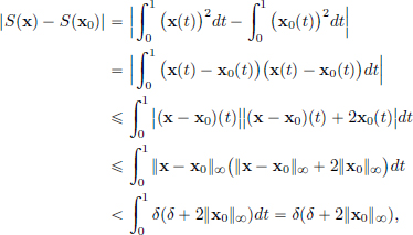
if ||x – x₀||_∞ < δ, where δ > 0 is some number. We ought to choose δ > 0 suitably so as to make the right-hand side above smaller than . There is no unique way to do this, and anything one can justify works. We set

Whenever ||x – x₀||_∞ < δ, in light of the above computation, we have

Thus S is continuous at x₀. As the choice of x₀ was arbitrary, it follows that S is continuous (on C[0, 1]).

Example 2.4. c₀₀ is the subspace of ℓ^∞ of all finitely supported sequences. c₀₀ is a normed space with the supremum norm inherited from ℓ^∞.

Consider the map s : c₀₀ → R given by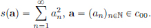

We’ll show that s is not continuous at 0. Suppose on the contrary that it is. With = 1/4 > 0, there exists a δ > 0 such that if ||a||_∞ = ||a – 0||_∞ < δ, then we are guaranteed that |s(a) – s(0)| = |s(a) – 0|= |s(a)| < = 1/4. If then So for all m sufficiently large, we must have ||a_m||_∞ < δ, giving in turn that |s(a_m)| < 1/4. But for all m we have

a contradiction. Hence s is not continuous at 0.

Exercise 2.3. (Rationale for the C¹[a, b] norm.)

This exercise concerns the norm on C¹[a, b] we have chosen to use. Since we want to be able to use ordinary analytic operations such as passage to the limit, then, given a function f : C¹[0, 1] → R, it is reasonable to choose a norm such that f is continuous. As our f, let us take the arc length function given by

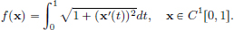
We show in the following sequence of exercises that f is not continuous if we equip C¹[0, 1] with the supremum norm || · ||_∞ induced from C[0, 1].

(1)Calculate f(0). (The arc length of the graph of the constant function taking value 0 everywhere on [0, 1] is obviously 1, and check that the above formula delivers this.)

(2)Now consider Using for all and the periodicity of sin(2πnt) (the graph of sin(2πnt) on is repeated n times in [0, 1]), conclude that

(3)Show that f is not continuous at 0. (Prove this by contradiction. Note that by taking larger and larger n, ||x_n – 0||_∞ can be made as small as we please, but f(xn) doesn’t stay close to f(0).)

Show that the arc length function f is continuous if we equip C¹[0, 1] with the norm || · ||_1,8. It may be useful to note that by using the triangle inequality in (R², || · ||₂), we have for a, b ∈ R that

Exercise 2.4. Let (X, || · ||) be a normed space. Show that the norm || · || : X → R is a continuous map.

Continuity and open sets

We’ll now learn an important property of continuous maps:

“inverse images” of open sets under a continuous map are open.

In fact, we shall see that this property is a characterisation of continuity. First let’s some notation. Let f : X → Y be a map between the normed spaces X and Y, and let V ⊂ Y. We set f^–1(V) := {x ∈ X : f(x) ∈ V}, and call it the inverse image of V under f. Clearly f^–1(Y) = X and f^–1(∅) = ∅.

Exercise 2.5. Let f : R → R be given by f(x) = cos x(x ∈ R).

Find f^–1(V), where V = {–1, 1}, V = {1}, V = [–1, 1], V = R,

On the other hand if U ⊂ X, then we set f(U) := {f(x) ∈ Y : x ∈ U}, and call it the image of U under f.

Exercise 2.6. Let f : R → R be given by f(x) = cos x (x ∈ R).

Find f(U), where U = R, U = [0, 2π], U = [δ, δ + 2π] where δ > 0.

Theorem 2.1. Let X, Y be normed spaces and f : X → Y be a map.

Then f is continuous on X if and only if

for every V open in Y, f^–1(V) is open in X.

Proof.

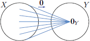
(If) Let c ∈ X, and let > 0. Consider the open ball B(f(c), ) with center f(c) and radius in Y . We know that this open ball V := B(f(c), ) is an open set in Y. Thus we also know that f^–1(V) = f^–1(B(f(c), )) is an open set in X. But the point c ∈ f^–1(B(f(c), )), because f(c) ∈ B(f(c), ) (||f(c), f(c)|| = 0 < !). So by the definition of an open set, there is a δ > 0 such that B(c, δ) ⊂ f^–1(B(f(c), )). In other words, whenever x ∈ X satisfies ||x – c|| < δ, we have x ∈ f^–1(B(f(c), )), that is, f(x) ∈ B(f(c), ), which implies ||f(x) – f(c)|| < . Hence f is continuous at c. But the choice of c ∈ X was arbitrary. Consequently f is continuous on X. See the picture on the left.

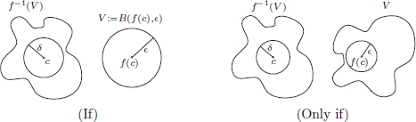
(Only if) Now let f be continuous, and let V be an open subset of Y. We would like to show that f^–1(V) is open. So let c ∈ f^–1(V. Then f(c) ∈ V. As V is open, there is a small open ball B(f(c), ) with center f(c) and radius that is contained in V. By the continuity of f at c, there is a δ > 0 such that whenever ||x – c|| < δ, we have ||f(x) – f(c)|| < , that is, f(x) ∈ V. But this means that B(c, δ) ⊂ f^–1(V). Indeed, if x ∈ B(c, δ), then ||x – c|| < δ and so by the above, f(x) ∈ V, that is, x ∈ f^–1(V). Consequently, f^–1(V) is open in X. See the picture on the right above.

Note that the theorem does not claim that for every U open in X, f(U) is open in Y. Consider for example X = Y = R equipped with the Euclidean norm, and the constant function f(x) = c (x ∈ R), which is clearly continuous. But note that direct images of open sets are not always open under f : indeed X = R is open in X = R, but f(X) = {c} is not open in Y = R.

Corollary 2.1. Let X, Y be normed spaces and f : X → Y be a map.

Then f is continuous on X if and only if

for every F closed in Y, f^–1(F) is closed in X.

Proof. If F ⊂ Y, then f^–1(Y\F) = X\(f^–1(F)).

Exercise 2.7. Fill in the details of the proof of Corollary 2.1.

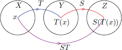
Theorem 2.2. Let X, Y, Z be normed spaces, and f : X → Y, g : Y → Z be continuous maps. Then the composition map g f : X → Z, defined by (g f)(x) := g(f(x)) (x ∈ X), is continuous.

Proof. Let W be open in Z. Then since g is continuous, g^–1(W) is open in Y. Also, since f is continuous, f^–1(g^–1(W)) is open in X. Finally, we note that (g f)^–1(W) = f^–1(g^–1(W)). So g f is continuous.

Exercise 2.8. In the proof of Theorem 2.2, we used (g f)^–1(W) = f^–1(g^–1(W)). Check this.

Exercise 2.9. Let X be a normed space and f : X → R be a continuous map. Determine if the following statements are true or false.

(1){x ∈ X : f(x) < 1} is an open set.

(2){x ∈ X : f(x) > 1} is an open set.

(3){x ∈ X : f(x) = 1} is an open set.

(4){x ∈ X : f(x) 1} is a closed set.

(5){x ∈ X : f(x) = 1} is a closed set.

(6){x ∈ X : f(x) = 1 or f(x) = 2} is a closed set.

(7){x ∈ X : f(x) = 1} is a compact set.

Continuity and convergence

We have the following characterisation of continuous maps in terms of convergence of sequences: “Continuous maps preserve convergent sequences”.

Theorem 2.3. Let X, Y be normed spaces, c ∈ X, and let f : X → Y. Then the following two statements are equivalent:

(1)f is continuous at c.

(2)For every sequence (x_n)_n∈N in X such that (x_n)_n∈N converges to c, (f(x_n))_n∈N converges to f(c).

Proof.

(1) ⇒ (2): Suppose that f is continuous at c. Let (x_n)_n∈N be a sequence in X such that (x_n)_n∈N converges to c. Let > 0. Then there exists a δ > 0 such that for all x ∈ X satisfying ||x – c|| < δ, we have ||f(x) – f(c)|| < . As the sequence (x_n)_n∈N converges to c, for this δ > 0, there exists an N ∈ N such that whenever n > N, ||x_n – c|| < δ. But then by the above, ||f(x_n) – f(c)|| < . So we have shown that for every > 0, there is an N ∈ N such that for all n > N, ||f(x_n) – f(c)|| < . In other words, the sequence (f(x_n))_n∈N converges to f(c).

(2) ⇒ (1): Suppose that f is not continuous at c. Thus there is an > 0 such that for every δ > 0, there is an x ∈ X such that ||x – c|| < δ, but ||f(x) – f(c)|| > . We will use this statement to construct a sequence (x_n)_n∈N for which the conclusion in (2) does not hold. Let δ = 1/n, for n ∈ N, and denote a corresponding x as x_n: thus, ||x_n – c|| < δ = 1/n, but ||f(x_n) – f(c)|| > . Clearly the sequence (x_n)_n∈N is convergent with limit c, but (f(x_n))_n∈N does not converge to f(c) since ||f(x_n) – f(c)|| > for all n ∈ N. Consequently if (1) does not hold, then (2) does not hold. In other words, we have shown that (2) ⇒ (1).

Exercise 2.10. Let X, Y be normed spaces. Find all continuous maps f : X → Y such that for all x ∈ X, f(x) + f(2x) = 0. Hint:

Exercise 2.11. (∗)(Continuity of the determinant; {invertible matrices} is open). Show that the determinant M → det M : (R^n×n, || · ||_∞) → (R, | · |) is continuous. Prove that the set of invertible matrices is open in (R^n×n, || · ||_∞). Hint: det^–1{0}.

Continuity and compactness

In this section we will learn about a very useful result in Optimisation Theory, on the existence of global minimisers of real-valued continuous functions on compact sets.

Theorem 2.4.

If(1)K is a compact subset of a normed space X,

(2)Y is a normed space, and

(3)f : X → Y is function that is continuous at each x ∈ K,
then f(K) is a compact subset of Y.

Proof. Suppose that (y_n)_n∈N is a sequence contained in f(K). Then for each n ∈ N, there exists an x_n ∈ K such that y_n = f(x_n). Thus we obtain a sequence (x_n)_n∈N in the set K. As K is compact, there exists a convergent subsequence, say (x_nk)_k∈N, with limit L ∈ K. As f is continuous, it preserves convergent sequences. So (f(x_nk))_k∈N = (y_nk)_k∈N is convergent with limit f(L) ∈ f(K). Consequently, f(K) is compact.

Now we prove the aforementioned result which turns out to be very useful in Optimisation Theory, namely that a real-valued continuous function on a compact set attains its maximum/minimum on the compact set. This is a generalisation of the Extreme Value Theorem we had learnt earlier, where the compact set in question was just the interval [a, b].

Theorem 2.5. (Weierstrass).

If(1)K is a nonempty compact subset of a normed space X, and

(2)f : X → R is a function that is continuous at each x ∈ K, then there exists a c ∈ K such that f(c) = sup{f(x) : x ∈ K}.

We note that since c ∈ K, f(c) ∈ {f(x) : x ∈ K}, and so the supremum above is actually a maximum:

Also, under the same hypothesis of the above result, there exists a minimiser in K, that is, there exists a d ∈ K such that

This follows from the above result by just looking at –f, that is by applying the above result to the function g : X → R given by g(x) = –f(x) (x ∈ X).

Proof. (Of Theorem 2.5.) We know that the image of K under f, namely the set f(K) is compact and hence bounded. So {f(x) : x ∈ K} is bounded. It is also nonempty since K is nonempty. But by the least upper bound property of R, a nonempty bounded subset of R has a least upper bound. Thus M := sup{f(x) : x ∈ K} ∈ R. Now consider M – 1/n (n ∈ N). This number cannot be an upper bound for {f(x) : x ∈ K}. So there must be an x_n ∈ K such that f(x_n) > M – 1/n. In this manner we get a sequence (x_n)_n∈N in K. As K is compact, (x_n)_n∈N has a convergent subsequence (x_nk)_k∈N with limit, say c, belonging to K. As f is continuous, (f(x_nk))_k∈N is convergent as well with limit f(c). But from the inequalities f(x_n) > M – 1/n (n ∈ N), it follows that f(c) M. On the other hand, from the definition of M, we also have that f(c) M. So f(c) = M.

Example 2.5. Since the set is compact in R³ and since the function x x₁ + x₂ + x₃ is continuous on R³, it follows that the optimisation problem

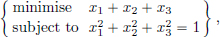
has a minimiser.

Remark 2.1. (∗) In Optimisation Theory, one often meets necessary conditions for a minimiser, that is, results of the following form:

(Here are certain mathematical conditions, such as the Lagrange multiplier equations.) Now such a result has limited use as such since even if we find all which satisfy , we can’t conclude that there is one that is a minimiser. But now suppose that we know that f is continuous on F and that F is compact. Then we know that a minimiser exists, and so we know that among the that satisfy , there is at least one which is a minimiser.

Notation 2.2. We will denote the set of all continuous maps from the normed space X to the normed space Y by C(X, Y).

2.3The normed space CL(X, Y)

In this section we study those linear transformations from a normed space X to a normed space Y that are also continuous.

Notation 2.3. We denote the set of all continuous linear transformations from the normed space X to the normed space Y by CL(X, Y), that is, CL(X, Y) := C(X, Y) ∩ L(X, Y). If X = Y, then we denote CL(X, X) simply by CL(X).

We begin by giving a characterisation of continuous linear transformations.

When is a linear transformation continuous?

Theorem 2.6.

Let X and Y be normed spaces, and T : X → Y be a linear transformation. Then the following properties of T are equivalent:

(1)T is continuous.

(2)T is continuous at 0.

(3)There exists an M > 0 such that for all x ∈ X, ||Tx||_Y M ||x||_X.

We’ll see the proof below. But let us first remark that the useful part is the equivalence of (1) and (3), since by just showing the existence/lack of of the bound M, we can conclude the continuity/lack of continuity of the given linear transformation. So we don’t have to go through the rigmarole of verifying the -δ definition: rather, a simple estimate, as stipulated in (3), suffices. Note also that it seems miraculous that continuity at just one point (at 0) delivers continuity everywhere on X! This miracle happens because the map T is not any old map, but rather a linear transformation. Here is an elementary example.

Example 2.6. (The left shift and right shift operators).

The left shift operator, L : ℓ² → ℓ², given by

is a linear transformation. We have for all (a_n)_n∈N ∈ ℓ² that

and so L ∈ C(ℓ², ℓ²). The right shift operator R : ℓ² → ℓ², given by R(a₁, a₂, a₃, ···) := (0, a₁, a₂, ···), (a_n)_n∈N ∈ ℓ², is also a linear transformation which is continuous, thanks to the equality

for all (a_n)_n∈N ∈ ℓ².

Proof. (Of Theorem 2.6.) We will show the three implications (1)⇒(2), (2)⇒(3), and (3)⇒(1), which are enough to get all the three equivalences (and six implications) given in the statement of the theorem.

(1)⇒(2). This is just the definition of continuity on X. Indeed, T has to be continuous at each point in X, and in particular at 0 ∈ X.

(2)⇒(3). Take := 1 > 0. Then there exists a δ > 0 such that whenever ||x – 0|| = ||x|| < δ, we have that ||Tx – T0|| = ||Tx – 0|| = ||Tx|| < 1. Let’s check that this yields:

First consider x = 0. Then

And so the claim in (2.2) holds because we have in fact an equality.

On the other hand, now suppose that x ≠ 0. Set Then

and so ||Ty|| < 1, that is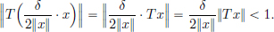

Upon rearranging, we obtain (2.2). So the claim in (3) holds with (3)⇒(1). Let M > 0 be such that for all x ∈ X, ||Tx|| M ||x||. Let x₀ ∈ X, and > 0. Set δ := /M > 0. Then whenever ||x – x₀|| < δ, we have

So T is continuous at x₀. But as x₀ ∈ X was arbitrary, T is continuous.

Example 2.7. (Norm on C¹[a, b] revisited). Consider the differentiation mapping D : C¹[0, 1] → C[0, 1] defined by (Dx)(t) = x′(t), t ∈ [0, 1], x ∈ C¹[0, 1]. We had seen that D is a linear transformation. Let’s now investigate if D is also continuous.

(1)We will show that D is not continuous if both C¹[0, 1] and C[0, 1] are equipped with the || · ||_∞ norm. Suppose on the contrary that the map D is continuous. Because D is a linear transformation, it follows from Theorem 2.6 that there exists an M > 0 such that for all x ∈ C¹[0, 1],

But if we take x = tⁿ (n ∈ N), then we have

and so ||Dx||_∞ = ||x′||_∞ = n M ||x||_∞ = M · 1, that is, n M for all n ∈ N, which is clearly not true. So D is not continuous.

(2)However, D is continuous if C¹[0, 1] is equipped with the || · ||_1,∞ norm:

while C[0, 1] has the usual supremum norm || · ||_∞. Indeed, we have for all x ∈ C¹[0, 1], that ||Dx||_∞ = ||x′||_∞ ||x||_∞ + ||x′||_∞ = ||x||_1,∞.

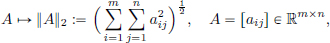
Example 2.8. (If X, Y are finite dimensional, then L(X, Y) = CL(X, Y).) Let X = (Rⁿ, || · ||₂), Y = (R^m, || · ||₂) and let A ∈ R^m×n be given by

Let T_A : Rⁿ → R^m be the linear transformation given by T_Ax := Ax for all x ∈ Rⁿ. Then for all x ∈ Rⁿ,

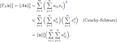
and so 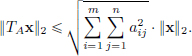Hence T_A is continuous.

Remark 2.2. We know that every linear transformation on finite dimensional vector spaces X, Y can be represented by T_A once bases for X, Y have been chosen. Also we know that all norms on finite-dimensional normed spaces are equivalent to each other. It follows from these two facts that every linear transformation between finite dimensional normed spaces is continuous.

Example 2.9. Let and let

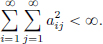
For x = (x_j)_j∈N ∈ ℓ², set

We claim that T_A : ℓ² → ℓ² is a continuous linear transformation on ℓ². Firstly, T_Ax ∈ ℓ², since

Moreover, it is easily seen that T_A ∈ L(ℓ²). Moreover, by Theorem 2.6, the computation above shows that T_A ∈ CL(ℓ²).

Example 2.10. (Integral operators).

Suppose that A : [0, 1] × [0, 1] → R be such that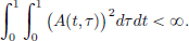

We think of A as a “non-discrete/continuous” analogue of a square matrix: the indices i, j are replaced by the “non-discrete/continuous” indices t, τ.

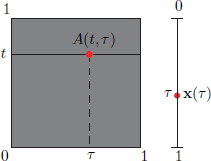
Then the map T_A : L²[0, 1] → L²[0, 1], defined by

is a continuous linear transformation. The following picture illustrates the action of T_A on x schematically, highlighting the analogy with matrix multiplication.

We note that for x ∈ L²[0, 1],

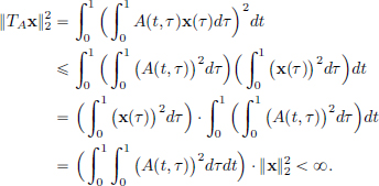
(The inequality in the second line above, is the Cauchy-Schwarz inequality in L²[0, 1], and it follows from the general Cauchy-Schwarz inequality in inner product spaces, which will be shown in Theorem 4.1, page 157; see also Example 4.3, page 159. We’ll accept this for now.) So T_Ax ∈ L²[0, 1], and T_A ∈ CL(L²[0, 1]).

Operators T_A are called integral operators. It used to be common to call the function A that plays the role of the matrix, as the “kernel”1 of the integral operator. Many variations of the integral operator are possible.

Example 2.11. We had seen on page 55 that with

and A, B ∈ C[a, b], the map L : S → R given by

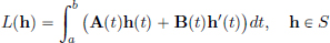
is a linear transformation. Now we ask: is L continuous? Here we equip S ⊂ C¹[0, 1] with the norm || · ||_1,∞. For h ∈ S,

where In the above, we have used

Hence L is continuous.

Example 2.12. (∗)(Fourier transform).

Let L¹(R) be the space of all complex valued Lebesgue integrable functions on R, with the usual L¹-norm:

Its Fourier transform is the function : R → C defined by

Then is a continuous function on R, and it is also bounded because

The vector space C_b(R) of all complex-valued continuous functions on R that are bounded, is a normed space with the supremum norm:

(We won’t check this; the proof is analogous to Example 1.9, page 10.) Thus from the above, we have ∈ C_b(R). It is also easy to check that : L¹(R) → C_b(R) is a linear transformation, and it is continuous, thanks to the estimate above, giving ||||_∞ ||f||₁.

Remark 2.3. Owing to the characterisation of continuous linear transformations by the existence of a bound as in item (3) of Theorem 2.6 above, they are sometimes called bounded linear operators.

Exercise 2.12. Show that if A ∈ R^m×n, then ker A = {x ∈ Rⁿ : Ax = 0} is a closed subspace of Rⁿ.

Exercise 2.13. (∗) Prove that every subspace of Rⁿ is closed.

Hint: Construct a linear transformation whose kernel is the given subspace.

Exercise 2.14. Let C[a, b] be endowed with the || · ||_∞-norm.

(1)Show that is a continuous linear transformation.

(2)Prove that if converges to f in C[a, b], then

Exercise 2.15. (Convolution operator).

If f ∈ L¹(R), then the corresponding convolution operator f∗ : L^∞(R) → L^∞(R) is given by

Show that f∗ is well-defined and that f∗ ∈ CL(L^∞(R)).

Exercise 2.16. Let Y = {f ∈ L²(R) : f = := f(–·)} be the set of all even functions in L²(R). Show that Y is a closed subspace of L²(R).

Hint: View Y as the kernel of a suitable map in CL(L²(R)).

Operator norm and the normed space CL(X, Y)

Consider the set CL(X, Y) of all continuous linear transformations from a normed space X to a normed space Y. We will show that CL(X, Y) is a normed space, with pointwise operations (inherited from L(X, Y)), and the “operator norm” || · || : CL(X, Y) → R given by

Let us first show that CL(X, Y) is a subspace of L(X, Y), making it a vector space in its own right.

Proposition 2.1. CL(X, Y) is a subspace of L(X, Y).

Proof. We have:

(S1)Let S, T ∈ CL(X, Y). Then there exist M_S, M_T > 0 such that for all x ∈ X, ||Sx|| M_S ||x|| and ||Tx|| M_T ||x||. So

Thus S + T ∈ CL(X, Y) too.

(S2)Let α ∈ R and T ∈ CL(X, Y). There exists an M > 0 such that for all x ∈ X, ||Tx|| M||x||. So ||(αT)x|| = ||α(Tx)|| = |α| ||Tx|| |α|M||x||. Hence αT ∈ CL(X, Y).

(S3)The zero linear transformation 0 ∈ CL(X, Y) because for all x ∈ X, ||0x|| = ||0_Y|| = 0 1 · ||x||.

Consequently, CL(X, Y) is a subspace of L(X, Y).

Next we show that the operator norm || · || : CL(X, Y) → R given by

is indeed a norm on CL(X, Y). First let us check that is a well-defined number. If we set S := {||Tx|| : x ∈ X, ||x|| 1}, then we note that this is a subset of the real numbers. Let us observe that this is a nonempty bounded set:

(1)S ≠ ∅ because if we take x = 0_X ∈ X, then ||x|| = ||0_X|| = 0 1, and so ||Tx|| = ||T0_X|| = ||0_Y|| = 0 ∈ S.

(2)S is bounded above. As T ∈ CL(X, Y), there is an M > 0 such that for all x ∈ X, ||Tx|| M||x||. We claim that M is an upper bound of S. Indeed, if x ∈ X and ||x|| 1, then ||Tx|| M||x|| M · 1 = M.

Since S is a nonempty subset of R which is bounded above, it follows from the Least Upper Bound Property of R that the supremum of S exists: so for all T ∈ CL(X, Y), ||T|| := sup{||Tx|| : x ∈ X, ||x|| 1} < ∞. In order to do our verification that this operator norm || · || is a norm on CL(X, Y), the following two results will be useful.

Lemma A. Let T ∈ CL(X, Y).

If M > 0 is such that for all x ∈ X, ||Tx|| M||x||, then ||T|| M.

Proof. If x ∈ X and ||x|| 1, then ||Tx|| M||x|| M · 1 = M. So M is an upper bound of S = {||Tx|| : x ∈ X, ||x|| 1}. Thus sup S M, that is, ||T|| M.

Lemma B. Let T ∈ CL(X, Y). Then for all x ∈ X, ||Tx|| ||T|| ||x||.

Proof.

1 x = 0. Then ||Tx|| = ||T0|| = ||0|| = 0 = ||T||0 = ||T|| ||0|| = ||T|| ||x||.

2 Suppose that 0_X ≠ x ∈ X. Let Then

Thus ||Ty|| ∈ S, and so ||Ty|| sup S = ||T||, that is,

Rearranging, we get ||Tx|| ||T|| ||x||.

Lemmas A and B together tell us that for a T ∈ CL(X, Y), ||T|| is allowed as an “M” in

and moreover it is the smallest possible such number M, in the sense that any other allowed M has got to be at least as large as ||T||.

Theorem 2.7. The operator norm, || · || : CL(X, Y) → R, given by

is a norm on CL(X, Y).

Proof. We have:

(N1)For T ∈ CL(X, Y), since ||Tx|| 0 for all x.

If T ∈ CL(X, Y) and ||T|| = 0, then ||Tx|| ||T|| ||x|| = 0||x|| = 0, and so ||Tx|| = 0, that is, Tx = 0_Y for all x ∈ X. So T = 0, the zero linear transformation.

(N2)For α ∈ K and T ∈ CL(X, Y),

(N3)Let T, S ∈ CL(X, Y). Then for all x ∈ X,

from which it follows (Lemma A) that ||T + S|| ||T|| + ||S||.

Example 2.13. Recall Example 2.8, page 69.

Let Rⁿ and R^m be equipped with the Euclidean || · ||₂-norm.

Let A = [A_ij] ∈ R^m×n, and T_A ∈ CL(Rⁿ, R^m) be the continuous linear transformation given by T_Ax = Ax, x ∈ Rⁿ.

Then we’d seen that for all x ∈ Rⁿ, So

So we have an estimate for ||T_A|| in terms of the matrix coefficients a_ij. But there does not exist a general “formula” for ||T_A|| in terms of the matrix coefficients except in the special cases n = 1 or m = 1, when ||T_A|| = |a₁₁|. It can be seen that the map

is also a norm on R^m×n, and is called the Hilbert-Schmidt norm of A.

Exercise 2.17. (Diagonal operator norm; operator norm needn’t be attained.) Let (λ_n)_n∈N be a bounded sequence in K, and let Λ ∈ CL(ℓ²) be given by Λ(a₁, a₂, a₃, ···) = (λ₁a₁, λ₂a₂, λ₃a₃, ···) for all (a₁, a₂, a₃, ···) ∈ ℓ². Show that Λ ∈ CL(ℓ²) and

Now let Show that there is no x ∈ ℓ² such that ||x||₂ 1 and ||Λx||₂ = ||Λ||. This gives an example showing that the operator norm need not be attained.

Exercise 2.18. (Schauder basis). Let X be a Banach space. A sequence of vectors (e_n)_n∈N in X is a Schauder basis for X if for every x ∈ X, there exists a unique sequence of numbers (ξ_n)_n∈N such that

Let 1 p < ∞, and e_n = (0, ···, 0, 1, 0, ···) be the sequence in ℓ^p with nth term equal to 1 and all others 0. Show that {e_n : n ∈ N} is a Schauder basis for ℓ^p.

Hint: For uniqueness use the continuity of the “coordinate map” φ_n : x x_n, selecting the nth term of the sequence x.

Remark. A Banach space X that has a Schauder basis is separable, that is, there exists a countable dense subset in X (for example the linear combinations of the e_n with rational coefficients). The converse of the above, namely if every separable Banach space had a Schauder basis, was an open problem for a long time. In 1973, the Swedish mathematician Per Enflo finally constructed an example of a separable Banach space that does not have a Schauder basis.

Exercise 2.19. (Invariant subspace, and the Invariant Subspace Problem)

(1)Prove that the averaging operator2 A : ℓ^∞ → ℓ^∞, defined by

is a continuous linear transformation. What is the operator norm of A?

(2)(∗) A subspace Y of a normed space X is said to be an invariant subspace with respect to a linear transformation T : X → X if TY ⊂ Y. Let A ∈ CL(ℓ^ℓ) be the averaging operator from part (1). Show that the subspace c of ℓ^∞, consisting of all convergent sequences, is an invariant subspace of the averaging operator A. Hint: Show that if x ∈ c has limit L, then Ax has limit L.

Remark. Invariant subspaces are useful since they are helpful in studying complicated operators by breaking them down into smaller operators acting on invariant subspaces. This is already familiar to the student from the diagonalisation procedure in linear algebra, where one decomposes the vector space into eigenspaces, and in these eigenspaces the linear transformation acts trivially. One of the open problems in functional analysis is the invariant subspace problem:

Does every T ∈ CL(H) on a separable complex Hilbert space H have a non-trivial invariant subspace?

Hilbert spaces are just special types of Banach spaces, in which the norm is induced by an inner product, and we will learn about Hilbert spaces in Chapter 4. Non-trivial means that the invariant subspace must be different from {0} or H. In the case of Banach spaces, the answer to the above question is “no”: during the annual meeting of the American Mathematical Society in Toronto in 1976, Per Enflo (again!) announced the existence of a Banach space and a bounded linear operator on it without any non-trivial invariant subspace.

Now that we know CL(X, Y) is a normed space with the operator norm, it is natural to ask if CL(X, Y) is complete, that is, if CL(X, Y) is a Banach space. It turns out that CL(X, Y) is a Banach space if and only if Y is a Banach space, and we’ll show this in the next section.

When is CL(X, Y) complete?

We’ll see that CL(X, Y) is a Banach space if and only if Y is a Banach space. In this section the “if” part will be shown, and the “only if” part will be done in Remark 2.9, page 109.

Theorem 2.8. If Y is a Banach space, and X is any normed space, then CL(X, Y) is a Banach space.

Proof. Let (T_n)_n∈N be a Cauchy sequence in CL(X, Y). Let x ∈ X. Claim: (T_nx)_n∈N is Cauchy in Y.

Indeed, for all n, m, ||T_nx – T_mx|| ||T_n – T_m|| ||x||.

As Y is Banach, (T_nx)_n∈N converges in Y, with limit, say Tx ∈ Y.

So we get a map x → Tx : X → Y.

Questions:(a)Is T ∈ CL(X, Y)?

(b)Does T_n T in CL(X, Y)?

(a)Is T a linear transformation?

If x₁, x₂ ∈ X, then (T_nx₁)_n∈N converges to Tx₁ in Y, and (T_nx₂)_n∈N converges to Tx₂ in Y. Thus (T_nx₁ + T_nx₂)_n∈N = (T_n(x₁ + x₂))_n∈N converges to Tx₁ + Tx₂ in Y. But we know that (T_n(x₁ + x₂))_n∈N converges to T(x₁ + x₂) in Y. By the uniqueness of limits, T(x₁ + x₂) = Tx₁ + Tx₂.

Let α ∈ K and x ∈ X. Then (T_nx)_n∈N converges to Tx in Y. So we have (α · (T_nx))_n∈N = (T_n(α · x))_n∈N converges to α · (Tx) in Y. But (T_n(α · x))_n∈N converges to T(α · x) in Y. So α · T(x) = T(α · x).

Is T continuous? Let = 1. Then there exists an N ∈ N such that for all n, m > N, ||T_n – T_m|| = 1. So for all n > N, ||T_n – T_N+1|| 1. Thus for n > N and x ∈ X, ||T_nx – T_{N +1}x|| ||T_n – T_N+1|| ||x|| 1 · ||x||. Passing the limit n → ∞, we obtain ||Tx – T_N+1x|| ||x|| for all x ∈ X. So for all x ∈ X, ||Tx|| ||Tx – T_N+1x|| + ||T_N+1x|| = (1 + ||T_N+1||) ||x||. Conclusion: T ∈ CL(X, Y).

(b)Is it true that T_n = T in CL(X, Y)?

Let > 0. Then there exists an N ∈ N such that for all n, m > N, we have ||T_n – T_m|| . So for all n, m > N and all x ∈ X, we obtain that ||T_nx – T_mx|| ||T_n – T_m || · ||x|| ||x||. Passing to the limit as m → ∞, we get that for all n > N and x ∈ X, ||T_nx – Tx|| ||x||. Hence for all n > N, ||T_n – T|| .

Corollary 2.2. If X is a normed space over K, then the dual space of X, X′ := CL(X, K), is a Banach space with the operator norm.

Corollary 2.3. If X is a Banach space, then CL(X) := CL(X, X) is a Banach space with the operator norm.

Remark 2.4. (“Hilbert” versus Banach spaces). In Chapter 4, we’ll meet Hilbert spaces: a Hilbert space is a special type of a Banach space in which the norm is induced by an “inner product”. If instead of Banach spaces, we are interested only in Hilbert spaces, then the notion of a Banach space is still indispensable, since for a Hilbert space H, the normed space CL(H) is typically only a Banach space, and not a Hilbert space in general.

(∗) Strong and weak operator topologies on CL(X, Y)

Many claims in this section won’t be proved, but are included to provide the reader with a “road map”. The main content of the section are the definitions of the three operator topologies and the illustrative examples. One who wants to know more could embark on a deeper study, as offered for example in [Pedersen (1989)] or [Rudin (1976)].

Let a set X be equipped with two topologies, and let X₁ (respectively X₂) denote the set X equipped with the first (respectively second) topology. If the identity map x → x : X₁ → X₂ is continuous, namely if every set open in X₂ is open in X₁, one says that first topology is stronger than the second, or that the second topology is weaker/coarser/smaller than the first. Of all the topologies on the set X, there is a strongest one (discrete topology), namely the one for which all subsets of X are open, and there is a weakest one (trivial topology), namely the one for which only X, ∅ are open.

Now suppose we have a set X, and a family F = {f_i : X → R | i ∈ I} of maps. Then of course there exists at least one topology on X with respect to which all the maps f_i are continuous, namely the discrete topology on X. However, there is also a “less wasteful/more efficient/weakest” topology on X that makes all the maps f_i, i ∈ I, continuous, characterized by the following: U is open in this topology on X if for every x ∈ U, there exist a finite number of indices i₁, ···, i_n ∈ I and intervals (a₁, b₁), ···, (a_n, b_n) such that x ∈ {y ∈ X : f_ik (y) ∈ (a_k, b_k), k = 1, ···, n} ⊂ U. It can be shown that this gives a topology T on X, and for any other topology T′ on X that makes the maps f_i, i ∈ I, continuous, we have T ⊂ T′.

We had seen that CL(X, Y) is a normed space with the operator norm ||T|| := sup{||Tx|| : x ∈ X, ||x|| 1}, T ∈ CL(X, Y). We call the resulting topology the uniform operator topology on CL(X, Y), and is the weakest topology making each map in the family

continuous. A subset U ⊂ CL(X, Y) is open in the uniform operator topology on CL(X, Y) if for each T ∈ U, there exists an > 0 such that {S ∈ CL(X, Y) : ||S – T|| < } ⊂ U. A sequence (T_n)_n∈N converges to T ∈ CL(X, Y) in the uniform operator topology if ||T_n – T|| = 0.

We remark that besides the uniform operator topology on CL(X, Y), there are weaker topologies (with fewer open sets), on CL(X, Y), called the Strong Topology and the Weak Topology. Here are the definitions, although in this basic introduction, we won’t use these useful alternative topologies much.

Definition 2.4. (Strong Operator Topology)

Let X, Y be normed spaces. Then the weakest topology on CL(X, Y) which makes each map in the family

continuous, is called the strong operator topology on CL(X, Y). A subset U ⊂ CL(X, Y) is open in the strong operator topology on CL(X, Y) if for each T ∈ U, there exists an > 0 and finitely many x₁, ···, x_n ∈ X such that {S ∈ CL(X, Y) : ||Sx_k – Tx_k|| < , k = 1, ···, n} ⊂ U. A sequence (T_n)_n∈N converges to T ∈ CL(X, Y) in the strong operator topology if for all x ∈ X, ||T_nx – Tx|| = 0.

Example 2.14. (Strong but not uniform convergence).

For n ∈ N, let P_n ∈ CL(ℓ²) be the “projection operator” given by

We claim that (P_n)_n∈N converges to the identity operator I ∈ CL(ℓ²) in the strong operator topology.

Indeed, ||Ia – P_na||₂² = ||(0, ···, 0, a_n+1, a_n+2, ···)||₂² =

But the sequence (P_n)_n∈N does not converge to the identity I ∈ CL(ℓ²) in the uniform operator topology. Let’s show this by contradiction.

Suppose it does converge to I with respect to the operator norm. With := 1/2 > 0, there exists an N ∈ N such that ||P_N – I|| < 1/2. So if e_N+1 ∈ ℓ² is the sequence with the (N + 1)st term 1 and all others 0, then we have

a contradiction!

A yet weaker topology than the strong operator topology is the weak operator topology, defined below.

Definition 2.5. (Weak Operator Topology)

Let X, Y be normed spaces. Let Y′ := CL(Y, K). Then the weakest topology on CL(X, Y) which makes each map in the family

continuous, is called the weak operator topology on CL(X, Y). A subset U ⊂ CL(X, Y) is open in the weak operator topology on CL(X, Y) if for all T ∈ U, there exists an > 0, finitely many x₁, ···, x_n ∈ X, and φ₁, ···, φ_n ∈ Y′ such that

A sequence (T_n)_n∈N converges to T ∈ CL(X, Y) in the weak operator topology if for all φ ∈ Y′ and for all

The following table summarises this:

Example 2.15. (Weak but not strong convergence).

Let R ∈ CL(ℓ²) be given by ℓ² ∋ (a₁, a₂, a₃, ···) (0, a₁, a₂, a₃, ···), the right shift operator. We claim that (Rⁿ)_n∈N converges to 0 ∈ CL(ℓ²) in the weak operator topology. We’ll use a result which will be proved later on in Theorem 2.14, page 104 (and also in Chapter 4, Theorem 4.10, page 189):

For each φ ∈ CL(ℓ², C) =: (ℓ²)′, there is an x_φ = (x_φ(k)_k∈N ∈ ℓ², such that

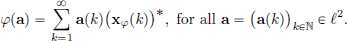
(Here ·^∗ denotes complex conjugation.)

Using the Cauchy-Schwarz inequality (page 159), for all a ∈ ℓ², φ ∈ (ℓ²)′,

Thus (Rⁿ)_n∈N converges to 0 ∈ CL(ℓ²) in the weak operator topology.

If e₁ := (1, 0, 0, ···) ∈ ℓ², then Rⁿe₁ = (0, ···, 0, 1, 0, ···), the sequence with (n + 1)st term 1 and all others 0. So ||Rⁿe₁||₂ = 1, n ∈ N. Thus it is not the case that Rⁿe₁ = 0 = 0e₁.

So (Rⁿ)_n∈N does not converge to 0 in the strong operator topology.

2.4Composition of continuous linear transformations

If T ∈ CL(X, Y),S ∈ CL(Y, Z), then the composition ST : X → Z of T, S is defined by (ST) (x) = S(T(x)), x ∈ X.

It is easily checked that ST is linear. Moreover, it is continuous too, since for all x ∈ X, we have ||(ST)(x)|| = ||S(T(x)) ||S|| ||Tx|| ||S|| ||T|| ||x||. Moreover, the above inequality shows that ||ST|| ||S|| ||T||.

In particular, if X is a normed space, then CL(X), besides possessing a natural addition and scalar multiplication (both defined pointwise), also possesses a natural multiplication of elements of CL(X), namely composition (S, T) ST : CL(X) × CL(X) → CL(X). So CL(X) is an “algebra”. Loosely speaking, an algebra is a vector space in which there is also available a nice way of multiplying vectors and producing new vectors.

Definition 2.6. (Algebra). An algebra is a vector space V in which an associative and distributive multiplication is defined, that is,

for all u, v, w ∈ V, and which is related to scalar multiplication so that

for all u, v ∈ V and all α ∈ K. We call e ∈ V a multiplicative identity element if for all v ∈ V, one has ev = v = ve.

The algebra V := CL(X) has a multiplicative identity element, namely the identity operator I. The identity operator is the map I : X X, given by Ix = x, x ∈ X. The operator I clearly belongs to CL(X) (with ||I|| = 1), and I serves as the multiplicative identity element of the algebra CL(X): IT = T = TI for all T ∈ CL(X).

Definition 2.7. (Normed and Banach algebras).

A normed algebra is an algebra V equipped with a norm || · || that satisfies:

A Banach algebra is a normed algebra which is complete.

We note that V := CL(X) is a normed algebra. We’d seen earlier that CL(X) is a Banach space if X is a Banach space. So CL(X) is a Banach algebra if X is a Banach algebra.

Let us note that as opposed to vector addition in CL(X), vector multiplication (that is, composition) in CL(X) is in general not commutative. Here is an example. Take X = R². Let T be clockwise rotation by π/2, and S be reflection in the x-axis, that is,

Then one can check that TS ≠ ST. This can also be observed visually by observing the distinct fates of the point (1, 0) under TS and under ST :

The commutator of A, B ∈ CL(X) is defined by [A, B] = AB – BA, and “measures” the lack of commutativity of A and B. The above example shows that the commutator may not be necessarily 0. In Exercise 2.22, page 86, we will investigate the “largeness” of the commutator in finite and infinite dimensional spaces X. This plays a role in Quantum Mechanics. We’ll show in Chapter 4 (page 204) that for “observables” A, B, the Heisenberg Uncertainty Relation holds:

We won’t explain this³ right now, but we simply notice that the commutator makes an appearance on the right-hand side.

If dim X = d < ∞, and T, S ∈ CL(X) are such that TS = I, then ST = I too. So TS = I ⇒ TS = ST = I. (Let us show this. First of all, if TS = I, then ker S = {0}. Indeed, if Sx = 0, then

Next observe that if {v₁, ···, v_d} is a basis for X, then {Sv₁, ···, Sv_d} are linearly independent: if α_ks are scalars such that α₁Sv₁ + ··· + α_dSv_d = 0, then S(α₁v₁ + ··· + α_dv_d) = 0, and so α₁v₁ + ··· + α_dv_d = 0, making all α_ks zeros. Hence {Sv₁, ···, Sv_d} must be a basis for X. For x ∈ X, there exist β_ks in K such that x = β₁Sv₁ + ··· + β_dSv_d = S(β₁v₁ + ··· + β_dv_d); and so STx = STS(β₁v₁ + ··· + β_dv_d) = SI(β₁v₁ + ··· + β_dv_d) = x.)

However, if dim X = ∞, then it can happen that TS = I, but ST ≠ I. Consider for example the left/right shift operators on ℓ². We have LR = I as LR(a₁, a₂, a₃, ···) = L(0, a₁, a₂, ···) = (a₁, a₂, ···) = I(a₁, a₂, a₃, ···), for all (a₁, a₂, a₃, ···) ∈ ℓ². But RL ≠ I since

This prompts the following definition.

Definition 2.8. (Invertible operator) Let X be a normed space. An element A ∈ CL(X) is said to be invertible if there exists a B ∈ CL(X) such that AB = I = BA.

Inverses are unique. This follows from the associativity of composition.

Proposition 2.2. If A ∈ CL(X) is invertible, then there exists a unique B ∈ CL(X) such that AB = I = BA.

The unique inverse of an invertible A ∈ CL(X) is denoted by A^–1 ∈ CL(X).

Proof. If B₁, B₂ ∈ CL(X) satisfy AB₁ = I = B₁A and AB₂ = I = B₂A, then B₁ = IB₁ = (B₂A)B₁ = B₂(AB₁) = B₂I = B₂.

Proposition 2.3. If A ∈ CL(X) is invertible, then A is bijective.

Proof. If x, y ∈ X are such that Ax = Ay, then A^–1(Ax) = A^–1(Ay), that is, Ix = Iy, and so x = y. Thus A is injective/one-to-one.

If y ∈ X, then x := A^–1 y ∈ X, and so Ax = A(A^–1y) = Iy = y. Hence A is surjective/onto too.

If A ∈ CL(X) is bijective, then the inverse map is automatically a linear transformation. In the case when dim X < ∞, we have L(X) = CL(X). So in this case the inverse is automatically continuous too. So if dim X < ∞, then A ∈ CL(X) is invertible if and only if A is a bijection.

In the infinite dimensional case, is it still true that if A ∈ CL(X) is a bijection, then A must be invertible? The answer is “yes” if X is a Banach space. The proof is not immediate, and we will show this below, using a deep result called the “Open Mapping Theorem”. But first, let us see an example showing that in non-Banach spaces, the inverses of continuous bijections may fail to be continuous.

Example 2.16. (Bijection, but not invertible.)

Recall that c₀₀ is the subspace of ℓ^∞ of all finitely supported sequences. Consider the map A : c₀₀ → c₀₀ given by

Then A is linear, and continuous (because ||Ax||_∞ ||x||_∞ for all x ∈ c₀₀). It is also easily seen that A is injective and surjective. So A is a bijection. However, it is not invertible. Indeed, if otherwise, B ∈ CL(c₀₀) is the inverse, then we would have, with e_m := (0, ···, 0, 1, 0, ···) (mth term 1, all others 0), that

giving m ||B|| for all m ∈ N, a contradiction. But we aren’t shocked by this example, since c₀₀ is not complete with the supremum norm, and the equivalence of bijectivity with invertibility is supposed to hold for operators in a Banach space.

Exercise 2.20. (When is the diagonal operator invertible?)

Let (λ_n)_n∈N be a bounded sequence in K, and consider Λ ∈ CL(ℓ²) given by

Show that Λ is invertible in CL(ℓ²) if and only if

Exercise 2.21. Let X be a normed space, and suppose that A, B ∈ CL(X).

Show that if I + AB is invertible, then I + BA is also invertible, with the inverse (I + BA)^–1 given by I – B(I + AB)^–1A.

Remark. This identity can be used to show that the nonzero spectrum of AB and BA coincide. λ is said to be in the spectrum of an operator T if λI – T is not invertible in CL(X).

Exercise 2.22. ([A, B] can’t be “large” for A, B ∈ CL(X).)

(1)The trace, tr(A), of a square matrix A = [a_ij] ∈ C^d×d is the sum of its diagonal entries: tr(A) = a₁₁ + ··· + a_dd. It can be shown that tr(A + B) = tr(A) + tr(B) and that tr(AB) = tr(BA). Prove that there cannot exist A, B in C^d×d such that AB – BA = I, where I denotes the d × d identity matrix.

(2)Let X be a normed space, and A, B be in CL(X). Show that if AB – BA = I, then for all n ∈ N, ABⁿ – Bⁿ A = nB^n–1, where we set B⁰ := I. Taking the operator norm on both sides of ABⁿ – Bⁿ A = nB^n–1, conclude that we can never have AB – BA = I with A, B ∈ CL(X).

(3)Let C^∞(R) denote the set of all functions f : R → R such that for all n ∈ N, f⁽ⁿ⁾ exists. It is clear that C^∞(R) is a vector space with pointwise operations. Consider the operators A, B : C^∞(R) → C^∞(R) given as follows:

(The operators A and B appear as the momentum operator and the position operator in Quantum Mechanics.) Show that AB – BA = I, where I denotes the identity on C^∞(R).

The Neumann Series Theorem.

Theorem 2.9. (Neumann4 Series Theorem).

Let X be a Banach space, and A ∈ CL(X) be such that ||A|| < 1.

Then (1) I – A is invertible in CL(X),

In particular, I – A : X → X is bijective: for each y ∈ X, there exists a unique solution x ∈ X of the equation x – Ax = y, and moreover,

so that x depends continuously on y.

This plays a role in integral equation theory:

where y, k are given, and x is the unknown function.

(This is called the Fredholm equation of the second type.)

Proof. (Of the Neumann Series Theorem). For all n ∈ N, ||Aⁿ|| ||A||ⁿ.

As ||A|| < 1, ||A||ⁿ converges. By comparison, ||Aⁿ|| converges too.

As X is Banach, so is CL(X). Since all absolutely convergent series in the Banach space CL(X) converge, it follows that

converges in CL(X). Is this S the inverse of I – A? For n ∈ N, define

Then we know that S_n = S in CL(X). We have

Since ||AS_n – AS|| ||A|| ||S_n – S|| and ||S_nA – SA|| ||A|| ||S_n – S||, it follows that SA = AS = S – I. This gives (I – A)S = I = S(I – A). Hence I – A is invertible in CL(X) and

Moreover,

Exercise 2.23. Consider the system

in the unknown variables (x₁, x₂) ∈ R². If I denotes the 2 × 2 identity matrix, then this system can be written as (I – K)x = y, where

(1)Show that if R² is equipped with the norm || · ||₂, then ||K|| < 1.
Conclude that (2.3) has a unique solution (denoted by x in the sequel).

(2)Find out the unique solution x by computing (I – K)^–1.

(3)Write a computer program to compute x_n = (I + K + ··· + Kⁿ)y and the relative error ||x – x_n||₂/||x||₂ for various values of n (say, until the relative error is less than 1%). Note the slow convergence of the Neumann series.

Exercise 2.24. Let X be a Banach space, and let A ∈ CL(X) be such that ||A|| < 1.

For n ∈ N, let P_n := (I + A)(I + A²)(I + A⁴) ··· (I + A²).

(1)Using induction, show that (I – A)P_n = I – A²ⁿ⁺¹ for all n ∈ N.

(2)Prove that (P_n)_n∈N is convergent in CL(X) to (I – A)^–1.

Exercise 2.25. (∗)(The set of invertibles is open, and ·^–1 is continuous.)

Let X be a Banach space and GL(X) denote the set of all invertible continuous linear transformations on X.

(1)Prove that GL(X) is an open subset of CL(X) in the usual operator norm topology.

(2)Prove that T T^–1 is continuous on GL(X), that is, for all T₀ ∈ CL(X) and each > 0, there exists a δ > 0 such that if T ∈ CL(X) satisfies ||T – T0|| < δ, then T ∈ GL(X) and ||T^–1 – T₀^–1|| < .

The exponential of an operator. Let X be a Banach space and let A ∈ CL(X). We will now study the exponential operator e^A ∈ CL(X).

For a ∈ R, one defines the exponential e^a ∈ R by

The exponential function e^· is useful, because it provides a solution to the initial value problem for the most basic differential equation

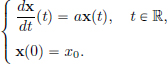
(Here x(t) ∈ R and x₀ ∈ R.) The unique solution is given by x(t) = e^tax₀, t ∈ R. This fundamental differential equation arises in all sorts of applications, for example, radioactive decay, Newton’s law of cooling, continuous compound interest, population growth, etc.

For A ∈ CL(X), we will show that an analogous definition,

(where we have simply replaced the little a by capital A!) works, and the series converges in CL(X). Then the map t e^tA x₀ provides a solution to the analogous initial value problem, but now in the Banach space X, with the initial condition x₀ ∈ X.

Theorem 2.10. Let X be a Banach space, and A ∈ CL(X).

Then 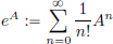converges in CL(X).

Proof. The real series converges (to e^||A||). Since for n ∈ N we have 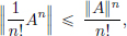by the Comparison Test, converges absolutely. So converges in the Banach space CL(X).

Remark 2.5. (∗) Recall that when a ∈ R, we have

Similarly, it can be shown that when A ∈ CL(X),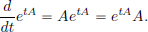

The last equality is not superfluous, since commutativity of multiplication in CL(X) is not always guaranteed, but it turns out that A does commute with e^tA. Formally, the above result is not surprising, as can be seen by differentiating the series for e^tA termwise with respect to t:

A rigorous justification can be given using the fact that e^(t+s)A = e^tA e^sA for all s, t ∈ R. In general, if A, B ∈ CL(X) commute, that is, AB = BA, then e^A+B = e^A e^B. This shows that e^A is always invertible in CL(X). Indeed, since A commutes with –A, we have e^–Ae^A = e^A–A = e⁰ = I = e^A e^–A.

Now let x₀ ∈ X, A ∈ CL(X), and consider the initial value problem:

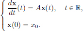
Then x(t) := e^tA x₀, t ∈ R, solves the initial value problem because

with x(0) = e^0Ax₀ = e⁰x₀ = Ix₀ = x₀.

Moreover, the solution is unique, since if is any solution, then

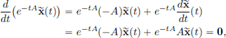
so that e^–tA(t) = e^–0A(0) = Ix₀ = x₀ for all t, giving

for all t ∈ R. Hence the solution t e^tA x₀, t ∈ R, is unique.

Initial value problems in Banach spaces of the above type arise from initial boundary value problems for partial differential equations and their discretisations. More generally, the operator A in the initial value problem is then “unbounded”, and similar to t e^tA, one can then associate a “C₀-semigroup generated by the infinitesimal operator A”. The solution to the initial value problem is given by x(t) = e^tA x₀ for t 0. For example, the initial value problem for the diffusion equation with the homogeneous Dirichlet boundary conditions

gives the initial value problem for the following ordinary differential equation in the Banach space L²[0, 1]:

where x(t) = u(·, t) ∈ L²[0, 1], and A : D(A)(⊂ L²[0, 1] → L²[0, 1] is an unbounded operator given by

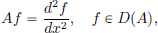
and

This completes our (rather long!) Remark 2.5.

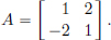
Example 2.17. (Computing e^A for diagonalisable A). Consider the system

With x = (x₁, x₂), this system can be written as x′(t) = Ax(t), where

We know that given the initial condition x₀ = (x₁(0), x₂(0)) ∈ R², the unique solution is x(t) = e^tAx₀. This raises the question:

There are several ways, but let us consider a method which works for diagonalisable As. First we note that if

and so

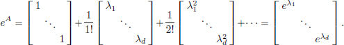
Note in particular that e⁰ = I, and so calculating e^A cannot be the same as taking exponentials of the entries of A!

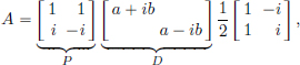
Now suppose that A is diagonalisable, that is, A = PDP^–1 where D is diagonal and P is invertible. Then Aⁿ = PDⁿP^–1 and so

Let’s see this method in action when where a, b ∈ R.

By computing the eigenvalues and eigenvectors of A, we can write

and so

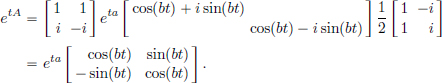
In particular, our initial value problem for (2.4) has the solution (putting a = 1 and b = 2 above)

So we’ve seen how to compute e^A if the matrix A is diagonalisable. However, not all matrices are diagonalisable. For example, consider the matrix

The eigenvalues of this matrix are both 0, and so if it were diagonalisable, say A = PDP^–1, then the diagonal matrix D must be the zero matrix. But then A = PDP^–1 = P0P^–1 = 0, and we have arrived at a contradiction since A ≠ 0! So this A is not diagonalisable.

In general, however, every matrix has what is called a Jordan canonical form, that is, there exists an invertible P such that P^–1AP = D + N, where D is diagonal, N is nilpotent (that is, there exists an n ∈ N such that Nⁿ = 0), and D and N commute. Then the exponential of A is:

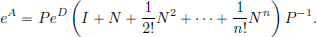
But the computation of a P taking A to its Jordan form requires some sophisticated linear algebra, and we won’t treat this here. The interested reader is referred to [Hirsch and Smale (1974), Chapter 6].

Exercise 2.26. (e^A+B ≠ e^A e^B).

Compute e^A and e^B, where A, B are the nilpotent matrices

Give an example of matrices A, B ∈ R^2×2 for which e^A+B ≠ e^A e^B.

2.5(∗) Open Mapping Theorem

In this section, we will show Theorem 2.11, the “Open Mapping Theorem”. The proofs in this section are somewhat more technical than the rest of the sections of this chapter.

Definition 2.9. (Open map) Let X, Y be normed spaces.

T ∈ CL(X, Y) is called open if for all open sets U ⊂ X, T(U) is open in Y.

Proposition 2.4.

Let X, Y be normed spaces, T ∈ CL(X, Y), and B := {x ∈ X : ||x|| 1}. Then the following are equivalent:

(1)T is open.

(2)There exists a δ > 0 such that B(0_Y, δ) ⊂ T(B).

Proof.

(2)⇒(1): Suppose that there exists a δ > 0 such that B(0_Y, δ) ⊂ T(B). Let U be open in X. If y₀ ∈ T(U), then y₀ = Tx₀ for some x₀ ∈ U. As U is open, there exists a r > 0 such that the open ball B(x₀, r) with centre x₀ and radius r is contained in U. We claim that the open ball B(y₀, δr/2) is contained in T(U). If y ∈ B(y₀, δr/2), then ||y – y₀|| < δr/2, that is, ||(2/r)(y – y₀)|| < δ, and so (2/r)(y – y₀) ∈ B(0_Y, δ) ⊂ T(B). Hence there exists an x ∈ B such that (2/r)(y – y₀) = Tx, that is, we have y = T((r/2)x + x₀). But as ||((r/2)x + x₀) – x₀|| = (r/2)||x|| (r/2) · 1 < r, we see that (r/2)x + x₀ ∈ B(x₀, r) ⊂ U. Consequently, y ∈ T(U), as desired.

(1)⇒(2): Suppose that T is open. Then T(B(0_X, 1)), the image of the open set B(0_X, 1), must be open. But 0_Y = T0_X ∈ T(B(0_X, 1)), and so, there must exist a δ > 0 such that the open ball B(0_Y, δ) ⊂ T(B(0_X, 1)) ⊂ T(B), as wanted. 0

Lemma 2.1. (Baire Lemma)

Let(1)X be a Banach space, and

(2)(F_n)_n∈N be a sequence of closed sets in X such that X = F_n.

Then there exist an n ∈ N and a nonempty open set U such that U ⊂ F_n.

Proof. We assume none of the sets F_n contain a nonempty open subset and construct a Cauchy sequence that converges to a point, which lies in none of the F_n, contradicting the fact that the F_ns cover X.

First let us observe that whenever a closed set F in X does not contain any open set, we have that F is dense in X. (To see this, let x ∈ X, and r > 0. We’d like to show that B(x, r) ∩ F ≠ ∅. If x ∈ F, then x ∈ B(x, r) ∩ F, and we are done. On the other hand, if x ∉ F, then x ∈ F. But as F doesn’t contain any open set, it won’t, in particular, contain B(x, r). So there must be an element y in B(x, r) which is not in F. But this means that y ∈ F, and so we’ve got y ∈ B(x, r) ∩ F, as wanted.) By our assumption, it follows that F_n is dense in X for all n ∈ N.

Let x₁ be any element in the nonempty (dense!) open set F₁. Let r₁ > 0 be such that ⊂ F₁. As F₂ is dense in X, there exists an x₂ ∈ B(x₁, r₁) ∩ F₂. As B(x₁, r₁) ∩ F₂ is open, we can find an r₂ < r₁/2 such that ⊂ B(x₁, r₁) ∩ F₂. As F₃ is dense in X, there exists an x₃ ∈ B(x₂, r₂) ∩ F₃. As B(x₂, r₂) ∩ F₃ is open, we can find an r₃ < r₁/4 such that ⊂ B(x₂, r₂) ∩ F₃.

Proceeding in this manner, we obtain a sequence (x_n)_n∈N, with the term x_n+1 ∈ B(x_n, r_n). If n > m, then B(x_n, r_n) ⊂ B(x_m, r_m), and so we have ||x_n – x_m|| < r_m < r₁/2^m–1 0. Thus (x_n)_n∈N is Cauchy, and as X is Banach, also convergent, say, to x ∈ X. With a fixed m, in the inequality above, if we pass the limit as n → ∞, then we obtain ||x – x_m|| r_m, that is, x ∈ ⊂ F_m. As the choice of m ∈ N was arbitrary, for all m ∈ N, x ∉ F_m. But this contradicts the fact that the F_ms cover X.

Exercise 2.27.

Show that the Hamel basis5 of a Banach space can only be finite or uncountable.

Before proving the Open Mapping Theorem, we’ll give some notation and a useful technical result. For subsets A, B of a normed space X and a scalar α, we set αA := {αa : a ∈ A}, and A + B := {a + b : a ∈ A, b ∈ B}.

Lemma 2.2. Let X be a normed space, and A ⊂ X satisfy

(1)A is symmetric, that is, –A = A,

(2)A is mid-point convex, that is, for all x, y ∈ A, ∈ A, and

(3)there is a nonempty open set U ⊂ A.

Then there exists a δ > 0 such that B(0, δ) ⊂ A.

Proof. First note that for a fixed scalar α ≠ 0, and an a ∈ X, the maps x x + a : X → X and x αx : X → X, are both continuous, with the continuous inverses (x x – a and x α^–1x).

Hence if U is open in X, then U + {–a} is open in X.

So U + (–A) = (U + {–a}) is open in X. Thus is open in X.

If a ∈ U, then 0 =

Thus there exists a δ > 0 such that B(0, δ) ⊂ .

Theorem 2.11. (Open Mapping Theorem).

Let X, Y be Banach spaces, and T ∈ CL(X, Y) be surjective.

Then T is open.

Proof. Let B := {x ∈ X : ||x|| 1}. Then X = nB. Thanks to the surjectivity of T, we have Y = T(nB). Thus certainly Y = T(nB). It can be checked that T(nB) = nT(B). By the Baire Lemma, there exists an n ∈ N such that nT(B) contains a nonempty open set. But since the map x nx : X → X is continuous with a continuous inverse, it follows that T(B) contains a nonempty open set too. By Lemma 2.2, there exists a δ > 0 such that B(0_Y, δ) ⊂ T(B). We will now show that this implies

giving the required openness of T by Proposition 2.4. Let y such that ||y|| < δ/2. We must show that there exists a x ∈ B with y = Tx. Using B(0_Y, δ) ⊂ T(B), it can be seen that

From (2.6), with n = 1, it follows that we can arbitrarily closely approximate y by elements from T(B/2). Thus there exists an x₁ with ||x₁|| 1/2 such that ||y – Tx₁|| δ/4 that is, y – Tx₁ ∈ B(0, δ/4). From (2.6) again it follows (with n = 2) that we can arbitrarily closely approximate y – Tx₁ by an element Tx₂ with ||x₂|| 1/4: ||y – Tx₁ – Tx₂|| δ/8. Proceeding in this manner, we can inductively construct a sequence (x_n)_n∈N such that: ||x_n|| 1/2ⁿ and ||y – Tx₁ – Tx₂ – ··· – Tx_n–1|| δ/2ⁿ.

As ||x_n|| x_n is absolutely convergent, and .

If we denote the sum of the series x_n by x, then

thanks to the continuity of T. Since ||x|| 1, this proves the desired inclusion (2.5).

Corollary 2.4. If X, Y are Banach spaces, and T ∈ CL(X, Y) is bijective, then T^–1 ∈ L(Y, X) is continuous.

We then refer to T as a normed space isomorphism, and say that X, Y are isomorphic (as normed spaces), written X Y.

Proof. T is open, and so if U is open in X, T(U) is open in Y. But (T^–1)^–1(U) = {y ∈ Y : T^–1y ∈ U} = {y ∈ Y : y ∈ T(U)} = T(U). Thus the inverse images of open sets under T^–1 are open, showing that T^–1 is continuous.

Exercise 2.28. Construct a continuous and surjective, but not open, f : R → R.

Exercise 2.29. (Closed Graph Theorem).

The aim of this exercise is to prove the Closed Graph Theorem:

Let X, Y be Banach spaces and T : X → Y be a linear transformation.

Then T is continuous if and only if its graph G(T) is closed in X × Y.

Here X × Y has the norm ||(x, y)} := max{||x||, ||y||}, (x, y) ∈ X × Y, and the set G(T) := {(x, Tx) : x ∈ X} ⊂ X × Y is the graph of T.

The “only if” part is easy to see. If (x_n, T_xn) → (x, y), then x_n → x, and as T is continuous, ||T_xn – Tx|| ||T|| ||x_n – x||, so that Tx_n → Tx. But Tx_n → y, and so, by the uniqueness of limits, Tx = y. Thus (x_n, Tx_n) → (x, Tx) ∈ G(T), showing that G(T) is closed.

Show the “if” part. Hint: Consider p : G(T) → X, where p((x, Tx)) = x, x ∈ X.

Uniform Boundedness Principle.

We give below another important application of the Baire Lemma.

Theorem 2.12. (Uniform Boundedness Principle).

Suppose that

(1)X and Y are Banach spaces,

(2)T_i ∈ CL(X, Y), i ∈ I, is a “pointwise bounded” family, that is,

Then the family is “uniformly bounded”, that is, ||T_i|| < + ∞.

Proof. For n ∈ N, F_n := {X ∈ X : ||T_ix|| n} = {x ∈ X : ||T_ix|| n} is mid-point convex, symmetric, and closed, as F_n is the intersection of the mid-point convex, symmetric, and closed sets {x ∈ X : ||T_ix|| n}, i ∈ I.

From (2), we have X = F_n, and so by the Baire Lemma, there exists an n such that F_n contains a nonempty open set. By Lemma 2.2, there exists a δ > 0 such that the ball B(0, δ) with center 0 and radius δ is contained in F_n, that is, if ||x|| < δ, then for all i ∈ I we have ||T_ix|| n. We claim that ||T_ix|| (2n/δ)||x|| for all x ∈ X and all i ∈ I. Clearly this is true if x = 0, since then both sides of the inequality are equal to 0. On the other hand, if x ≠ 0, then y := x has norm ||y|| = δ/2 < δ, and so we must have ||T_iy|| n, which, using the linearity of T_i and the positive homogeneity of the norm, delivers, upon a rearrangement, the desired inequality. Thus ||T_i|| 2n/δ for all i ∈ I, and thus ||T_i|| 2n/δ.

Corollary 2.5. (Banach-Steinhauss Theorem).

Let(1)X, Y be Banach spaces, and

(2)(T_n)_n∈N in CL(X, Y) be such that T_nx exists for all x ∈ X.

Then x T_nx : X → Y belongs to CL(X, Y).

Proof. It is clear that the map x T_nx : X → Y is linear.

It remains to show that it is continuous too. Set Tx := T_nx, x ∈ X. For each x ∈ X, (T_nx)_n∈N is convergent, and in particular, bounded:

Hence by the Uniform Boundedness Principle, there exists an M such that for all n ∈ N, ||T_n|| M. This gives, for each fixed x ∈ X, that

Passing the limit n → ∞ yields ||Tx|| M||x||. As the choice of x was arbitrary, this holds for all x, and consequently, the linear transformation T is continuous.

2.6Spectral Theory

For a linear transformation T ∈ L(X) on a finite dimensional vector space X over C, the set of eigenvalues of T is known as its spectrum σ(T), and has cardinality at most dim X. But in infinite dimensional complex vector spaces, strange things may happen, for example linear transformations may have no eigenvalues at all or finitely many or (countably/uncountably) infinitely many! First of all, here is a natural definition of eigenvectors and eigenvalues, extending our prior familiarity with eigenvalues from elementary linear algebra. We remind the reader that the prefix eigen is derived from German, meaning “one’s own”.

Definition 2.10. (Eigenvalues and eigenvectors). Let X be a normed space and T ∈ CL(X). Then λ ∈ C is called an eigenvalue of T if there exists a nonzero vector x ∈ X such that Tx = λx. Such a nonzero vector x is then called an eigenvector of T corresponding to the eigenvalue λ.

Example 2.18. (Uncountably many eigenvalues).

Let λ ∈ D := {z ∈ C : |z| < 1}. If x := (1, λ, λ², λ³, ···), then as |λ| < 1,

and so x ∈ ℓ². Clearly x ≠ 0 too.

We see that x is an eigenvector of the left shift operator L ∈ CL(ℓ²) because

Thus each point in the open unit disk6 is an eigenvalue of L.

Example 2.19. (No eigenvalues). On the other hand, the right shift operator R ∈ CL(ℓ²) has no eigenvalues. Suppose that λ ∈ C is such that Rx = λx for some x = (x_n)_n∈N ∈ ℓ². Then

Suppose first that λ ≠ 0. Then from the above, λx₁ = 0 gives x₁ = 0. Next, λx₂ = x₁ now gives x₂ = 0. Proceeding in this manner, we obtain x₁ = x₂ = x₃ = ··· = 0, and so x = 0.

On the other hand, if λ = 0, then (0, x₁, x₂, x₃, ···) = (λx₁, λx₂, λx₃, ···) shows immediately that x₁ = x₂ = x₃ = ··· = 0, and so x = 0.

Consequently, R has no eigenvalues.

Note that when dim X < ∞, and T ∈ CL(X), then

λ ∈ C is an eigenvalue of T if and only if λI – T is not invertible.

So the points in the spectrum σ(T) are exactly the ones where λI – T fails to be invertible in σ(T). This prompts the following natural concept in the general case, that is, when dim X ∞.

Definition 2.11. (Spectrum and resolvent).

Let X be a normed space and T ∈ CL(X).

We say that λ ∈ C belongs to the spectrum σ(T) of T if λI – T is not invertible in CL(X). Thus

The set ρ(T) is called the resolvent set of T.

The set σ_p(T) of all eigenvalues of T is called the point spectrum of T.

We have that σ_p(T) ⊂ σ(T), since if λ ∈ σ_p(T), then there exists a nonzero vector x such that Tx = λx, that is, (λI – T)x = 0, showing that λI – T is not injective, and hence can’t be invertible either!

We’ll now show that if X is Banach and T ∈ CL(X), then σ(T) is a compact nonempty subset of C.

Theorem 2.13. Let X be a Banach space and T ∈ CL(X).
Then

(1)σ(T) ⊂ {λ ∈ C : |λ| ||T||}.

(2)ρ(T) is an open subset of C.

(3)σ(T) is a compact subset of C.

(4) σ(T) is nonempty.

Proof.

(1)Let |λ| > ||T|| 0. Then < 1, and so I – is invertible in CL(X). Thus, as λ ≠ 0, we have that

is invertible in CL(X) too.

(2)Let λ₀ ∈ ρ(T). Then for λ ∈ C,

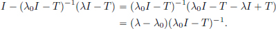
So I – .

For λ₀ ≈ λ, A has small norm, in particular, < 1. Hence it follows that (λ₀I – T)^–1(λI – T) =: S is invertible in CL(X). So we conclude that λI – T = (λ₀I – T)S (being the product of two invertible operators in CL(X)) is also invertible in CL(X).

(3)σ(T) is bounded (as σ(T) ⊂ B(0, ||T||) := {z ∈ C : |z| ||T||}), and also it is closed (because its complement C\σ(T) = ρ(T) is open). So σ(T) is compact.

(4)(∗)7 Let σ(T) = ∅. Then f(z) := (zI – T)^–1 ∈ CL(X) for all z ∈ C.

In particular, T^–1 exists, and is not 0.

Let φ ∈ (CL(X))′ be such that φ(T^–1) ≠ 0.

Such a φ exists by the Hahn-Banach Theorem (Exercise 2.38, page 109).

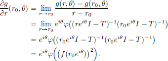
Let g : R² → C be given by g(r, θ) = φ(f(re^iθ)), for all (r, θ) ∈ R².

We will show that g ∈ C¹ (R², C) by showing that it has continuous first order partial derivatives (which will in turn be used in the calculations, and also to justify a differentiation under the integral sign).

Using the resolvent identity (Exercise 2.30, page 102), we have

Using continuity of φ and that of the inverse operation (Exercise 2.25, page 88), it follows from the above calculation, that

Similarly, .

By differentiating under the integral sign, we obtain

Consequently,

Hence F is constant, and we have

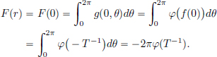
Now

Fix r such that |φ(f(re_iθ))| < . Then

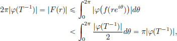
giving 2 < 1, a contradiction. This completes the proof.

Example 2.20. (Spectrum of the left shift operator).

Consider the left shift operator L ∈ CL(ℓ²). Then ||L|| 1. So it follows that σ(L) ⊂ {z ∈ C : |z| 1}. As {z ∈ C : |z| < 1} ⊂ σ_p(L) ⊂ σ(L), and because σ(L) is closed, it follows that {z ∈ C : |z| 1} ⊂ σ(L) too. So σ(L) = {z ∈ C : |z| 1}.

We now claim that σ_p(L) = {z ∈ C : |z| < 1}. We had seen earlier that {z ∈ C : |z| < 1} ⊂ σ_p(L). Now we’ll show the reverse inclusion.

To this end, let λ ∈ σ_p(L) with eigenvector x = (x_n)_n∈N.

Then (x₂, x₃, ···) = L(x₁, x₂, x₃, ···) = λ(x₁, x₂, x₃, ···).

So λx_n = x_n+1 for all n, giving (by induction) x_n = λ^n–1x₁ for all n.

As ℓ² ∋ x ≠ 0, we have

so that x₁ ≠ 0, and the geometric series with common ratio |λ|² converges. So |λ| < 1, and we get the reverse inclusion σ_p(T) ⊂ {z ∈ C : |z| < 1}.

We will return to this topic on spectral theory when we deal with operators on a Hilbert space, and also in the context of compact operators.

Exercise 2.30. (Resolvent Identity). Let X be a normed space, T ∈ CL(X) and λ, μ ∈ ρ(T). Prove that (λI – T)^–1 – (μI – T)^–1 = (μ – λ)(λI – T)^–1(μI – T)^–1.

Exercise 2.31. (Spectral radius). Let X be a Banach space, and T ∈ CL(X). Define the spectral radius of T by r_σ(T) := |λ|.

(1)Prove that r_σ(T) ||T||.

(2)Show that for T_A ∈ CL(R²), A := , then r_σ(T_A) < ||T_A||.

Here R² has the usual Euclidean || · ||₂-norm.

Remark. In this connection, the Gelfand-Beurling Formula8 says that:

If X is Banach and T ∈ CL(X), then r_σ(T) = ||Tⁿ||^1/n.

Exercise 2.32. Let X be a Banach space, T ∈ CL(X), and λ ∈ σ(T).

Prove that λ² belongs to the spectrum of T².

Hint: Use (λ²I – T²) = (λI – T)(λI + T) = (λI + T)(λI – T).

Remark. More generally, the Spectral Mapping Theorem9 says that:

If X is a Banach space, T ∈ CL(X), p = c₀ + c₁z + · · · + c_dz^d ∈ C[z] (a polynomial with complex coefficients), and p(T) := c₀I + c₁T + · · · + c_dT^d, then we have σ(p(T)) = p(σ(T)) := {p(λ) : λ ∈ σ(T)}.

Exercise 2.33. (Spectrum of the diagonal operator).

Let (λ_n)_n∈N be sequence in C which is convergent to 0, and consider Λ ∈ CL(ℓ²) given by Λ(a₁, a₂, a₃, · · ·) = (λ₁a₁, λ₂a₂, λ₃a₃, · · ·) for all (a₁, a₂, a₃, · · ·) ∈ ℓ².

Show that {λ_n : n ∈ N) ⊂ σ_p(Λ) ⊂ {λ_n : n ∈ N) {0} = σ(Λ).

Remark. (Spectral Theorem for Compact Operators).

In Chapter 5, we will learn that this Λ is an example of a “compact operator”; see Example 5.3 on page 214. More generally, one can show the Spectral Theorem for Compact Operators, which says that for a compact operator K on an infinite dimensional Hilbert space H,

(1)σ(K\{0} = σ_p(K\{0}, and σ(K) is countable,

(2)0 is the only accumulation point of σ(K),

(3)For all λ ∈ σ_p(K\{0}, dim kerp(λI – K) = dim kerp(λ*I – K*) < ∞.

Exercise 2.34. (Approximate spectrum).

(1)Let X be a Banach space, and T ∈ CL(X). A number λ ∈ C is said to belong to the approximate spectrum σ_ap(T) of T if there exists a sequence (x_n)_n∈N of vectors from X such that ||x_n|| = 1 for all n ∈ N, and Tx_n – λx_n 0 in X. Prove that σ_ap(T) ⊂ σ(T).

(2)Let Λ ∈ CL(ℓ²) be the diagonal operator corresponding to a convergent (and hence bounded) sequence (λ_n)_n∈N. Prove that λ_n ∈ σ_ap(Λ).

Exercise 2.35. (Point spectrum of the position operator).

Let X be a normed space, and let A : D_A → X be an “unbounded operator¹⁰”, where the domain D_A is a subspace of X. Then the point spectrum of the unbounded operator A is defined in an analogous manner as before: σ_p(A) := {λ ∈ C : there exists an x ∈ D_A\{0} such that Ax = λx}.

Now consider the position operator Q : D_Q → L²(R), arising in Quantum Mechanics, where D_Q := {Ψ ∈ L²(R) : (x → xΨ(x)) =: QΨ ∈ L²(R)}, and (QΨ)(x) := xΨ(x), for almost all x ∈ R, and all Ψ ∈ D_Q.

Show that σ_p(Q) = ∅.

Remark. So Q has no eigenvectors in D_Q ⊂ L²(R). However, when we learn elementary distribution theory later on in Chapter 6, we’ll see that xδ_λ = λδ_λ for all λ ∈ R, where δ_λ is the “Dirac distribution” with support at λ ∈ R. See Example 6.11 on page 251.

2.7(∗) Dual space and the Hahn-Banach Theorem

Definition 2.12. (Dual space of a normed space).

Let X be a normed space over K. Then the normed space CL(X, K), equipped with the operator norm, is called the dual space of X. One denotes the dual space of X simply by X′. Elements of the dual space are sometimes called bounded linear functionals.

Recall that a consequence of Theorem 2.8 (page 78) was Corollary 2.2, which says that X′ is always a Banach space, even if X isn’t. This is because K = R or C are both Banach spaces.

Given a concrete X, like R^d or ℓ^p, it is sometimes possible to “recognize” X′, that is to establish a (normed space) isomorphism from X′ to some other Banach space, for example:

Such results are called representation theorems, and we will see a few such results now, and also later on in the chapter on Hilbert spaces (Chapter 4), when we will learn about the Riesz Representation Theorem, page 189.

Theorem 2.14. For 1 p < ∞, (ℓ^p)′ » ℓ^p, where

(Here the understanding is that if p = 1, then q = ∞.)

Proof. (Sketch). We consider K = R for simplicity. Let 1 < p < ∞.

By Hölder’s Inequality, |a₁b₁ + · · · + a_nb_n| ||(a₁, · · ·, a_n)||_p||b₁, · · ·, b_n)||_q, with equality if is a multiple of . Let T ∈ CL(ℓ^p, R). Let e_k ∈ ℓ^p be the sequence (0, · · ·, 0, 1, 0, · · ·) with kth term 1, and all others 0. Fix n ∈ N. Let a = (a₁, · · ·, a_n, 0, · · ·) ∈ ℓ^p be such that is a multiple of ((Te₁)^q, · · ·, (Te_n)^q) (i.e., a_k := (Te_k)^p/q, k = 1, · · ·, n).

Then ||T|| = ||(Te₁, · · · , Te_n)||_q.

Passing the limit n → ∞, we get (Te₁, Te₂, Te₃, · · ·) ∈ ℓ^q. So we get a continuous linear transformation T (Te₁, Te₂, Te₃, · · ·) : CL(ℓ^p, R) → ℓ^p. It can be checked that this map ι is injective and surjective. As ι is bijective, it is an isomorphism.

If p = 1, then let us now show that (ℓ¹)′ ℓ^∞. This is easier to see, since if T ∈ CL(ℓ¹, R), then we get immediately that for all k, |Te_k| = ||T||, giving (Te_k)_k∈N ∈ ℓ^∞.

Remark 2.6. (The dual space (ℓ^∞)′ ℓ′.)

If a = (a_n)_n∈N ∈ ℓ¹, then define the functional φ_a ∈ CL(ℓ^∞, R) = (ℓ^∞)′ by

Then a φ_a : ℓ¹ → (ℓ^∞)′ is an injective linear transformation. It is continuous since |φ_a(b)| ||b||_∞||a||₁ for all b ∈ ℓ^∞, giving ||φ_a|| ||a||₁. However it is not surjective, and this can be shown by using the Hahn-Banach Theorem (see Theorem 2.15 on page 108), which says that a continuous linear functional on a subspace of a normed space can be extended to the whole normed space while preserving the operator norm of the functional. To see how this gives the non-surjectivity of the map a φ_a : ℓ¹ → (ℓ^∞)′ above, let us consider the subspace c ⊂ ℓ^∞ of all convergent subsequences, and the “limit functional” λ : c → R, given by

Then λ ∈ CL(c, R) = c′, and ||λ|| = 1. By the Hahn-Banach Theorem, this functional λ on the subspace c of ℓ^∞ has an extension Λ ∈ CL(ℓ^∞, R). But now we see that Λ can’t be φ_a for some a ∈ ℓ¹. Otherwise, with e_n ∈ c ⊂ ℓ^∞ being the sequence with nth term 1 and all others 0, we have

for all n, showing that a = 0, and so Λ = φ_a = 0, which is clearly false, since Λ(1, 1, 1, · · ·) = λ(1, 1, 1, · · ·) = 1 ≠ 0! So (ℓ^∞)′ is “bigger” than ℓ¹.

Remark 2.7. If 1 p < ∞, then it can be shown that

where

Exercise 2.36. Consider the subspace c₀ ⊂ ℓ^∞ consisting of all sequences that converge to 0. Prove that ℓ¹ (c₀)′.

Exercise 2.37. (∗) (Dual of C[a, b]). In this exercise we will learn a representation of the dual space of C[a, b]. A function μ : [a, b] → R is said to be of bounded variation on [a, b] if its total variation var(μ) on [a, b] is finite, where

Here P is the set of all partitions of [a, b]. A partition of [a, b] is a finite set P = {t₀, t₁, · · ·, t_n–1, t_n} with t₀ := a < t₁ < · · · < t_n–1 < b =: t_n.

(1)Show that the set of all functions of bounded variations on [a, b], with the usual pointwise operations forms a vector space, denoted BV[a, b].

Define || · || : BV[a, b] → [0, +∞) by ||μ|| := |μ(a)| + var(μ), for μ ∈ BV[a, b].

(2)Prove that || · || is a norm on BV[a, b].

The Riemann-Stieltjes integral: Let x ∈ C[a, b] and μ ∈ BV[a, b]. For a partition of [a, b], say P = {t₀, t₁, · · ·, t_n–1, t_n}, let δ_P be the length of a largest interval [t_j–1, t_j], that is, δ_P := max{t₁ – t₀, · · ·, t_n – t_n–1}, and set

Then it can be shown that there exists a unique real number, denoted by

called the Riemann-Stieltjes integral of x over [a, b] with respect to μ, such that for every > 0 there is a δ > 0 such that if P is a partition of [a, b] satisfying δ_P < δ, then

The usual linearity of the integral (as with the ordinary Riemann integral) holds:

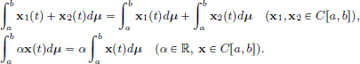
(3)Prove that ||x||_∞ var(μ), where x ∈ C[a, b] and μ ∈ BV[a, b].

(4)Conclude that every μ ∈ BV[a, b] gives rise to a φ_µ ∈ CL(C[a, b], R),

and that ||φ_µ|| var(μ).

The following converse result was proved by F. Riesz: For all φ ∈ CL(C[a, b], R), there exists a μ ∈ BV[a, b] such that

and ||φ|| = var(μ). In other words, every element (C[a, b]′ can be represented by a Riemann-Stieltjes integral.

(5)For the functional x x(a) on C[a, b], find a corresponding μ ∈ BV[a, b].

Dual spaces are important because, among other things, they allow us to define dual operators. Here is the definition.

Definition 2.13. (Dual operator).

Let X, Y be normed spaces, and T ∈ CL(X, Y). We define the dual operator (of T), T′ ∈ CL(Y′, X′), by (T′ψ)(x) = ψ(Tx), for all x ∈ X and ψ ∈ Y′.

Several things need to be checked here:

(1)For ψ ∈ Y′, does T′ψ belong to X′?

(2)Does T′ ∈ CL(Y′, X′)?

Let us begin with (1). If ψ′ ∈ Y′, then we have that

(L1)for all x₁, x₂ ∈ X,

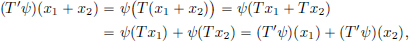
(L2)for all α ∈ K and x ∈ X,

Hence T′ψ ∈ L(Y, K). Moreover T′ψ is continuous because for all x ∈ X,

Now let’s check (2), that is, that T′ ∈ CL(Y′, X′). We have

(L1)for all ψ₁, ψ₂ ∈ Y′, for all x ∈ X,

and so T′(ψ₁ + ψ₂) = T′(ψ₁) + T′(ψ₂),

(L2)for all α ∈ K, for all ψ ∈ Y′, for all x ∈ X,

and so T′(αψ) = α(T′ψ).

Thus T′ is linear. It is also continuous, because (2.7) gives ||T′ψ|| ||ψ||||T|| for all ψ, that is T′ ∈ CL(Y′, X′) and ||T′|| ||T||.

Example 2.21. Consider x x′ : C¹[0, 1] → C[0, 1], x ∈ C¹[0, 1]. Then D′ : (C[0, 1]) → (C¹[0, 1])′ is given by (D′ψ)(x) = ψ(Dx) = ψ(x′), ψ ∈ (C[0, 1])′, x ∈ C¹[0, 1]. But (C[0, 1])′ ⊂ BV[0, 1], and so every ψ ∈ (C[0, 1])′ can be represented by some element μ_ψ ∈ BV[0, 1], so that

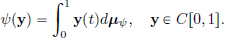
Thus if ψ ∈ (C[0, 1])′, then

where μ_ψ ∈ BV[0, 1] is such that ψ(y) = y(t)dμ_ψ, y ∈ C[0, 1].

Sometimes problems for an operator can be simplified by looking at the dual operator, making the consideration of dual spaces and dual operators a useful endeavour.

Remark 2.8. (Dual versus adjoint operators). When we learn about Hilbert spaces, we will learn about the notion of the adjoint T* ∈ CL(Y, X) of an operator T ∈ CL(X, Y), where X, Y are Hilbert spaces, and we can use the Riesz Representation Theorem (which we will also learn there) to represent elements of Y′, X′ by elements of Y, X. (The next sentence should be read after the discussion of the adjoint operator and the Riesz Representation Theorem.) If X, Y are Hilbert spaces, and T ∈ CL(X, Y), then for Y ∋ y_ψ ≡ ψ ∈ Y′, we have for all x ∈ X that

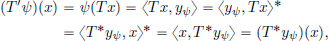
where we identified T*y_ψ ∈ X with the functional x → 〈x, T*y_ψ〉 : X → K in X′. In this sense the notions of adjoint and dual “coincide” in this context of operators on Hilbert spaces.

Hahn-Banach Theorem11. Finally, we will learn a fundamental result, known as the Hahn-Banach Theorem, which says that X′ always contains sufficiently many elements to separate points of X : for x ≠ y in X, there exists a φ ∈ X′ such that φ(x) ≠ φ(y). In this sense, the elements of X′ play the role of “coordinates” for the points of X (which is the kind of thinking one is used to in elementary linear algebra when X = K^d).

Theorem 2.15. (Hahn-Banach).

Let (1) X be a normed space,

(2)Y ⊂ X be a linear subspace,

(3)φ ∈ CL(Y, K).

Then there exists a Φ ∈ CL(X, K) such that Φ|_Y = φ and ||Φ|| = ||φ||.

In other words: “Every continuous linear functional on a subspace Y of a normed space X possesses a norm-preserving extension to the entire normed space X”.

Before proving the Hahn-Banach Theorem, we will now list a few important consequences one obtains from it.

Corollary 2.6. Let X be a normed space and x₀ ∈ X. Then there exists an element Φ ∈ X′ such that Φ(x₀) = ||x₀|| and ||Φ|| = 1.

Proof. Let Y := span {x₀} and φ : Y → K be given by φ(y) = α||x₀|| for y = αx₀ ∈ Y, α ∈ K. Then φ is linear. Moreover, φ is a continuous map because |φ(y)| = |φ(αx₀)| = |α||x₀||| = ||αx₀|| = ||y||, that is, |φ(y)| = ||y|| for all y ∈ Y. Hence ||φ|| = 1. By Hahn-Banach there now exists an extension Φ with the desired property.

As mentioned earlier, once we have the Hahn-Banach Theorem, one has the ability of distinguishing elements of X using elements from X′. This is shown in the two corollaries below.

Corollary 2.7. Let x and y be elements in a normed space X with x ≠ y. Then there exists a Φ ∈ X′ such that Φ(x) ≠ Φ(y). (In other words, X′ separates the points of X.)

Proof. Take Φ ∈ X′ with Φ(xq– Φ(y) = Φ(x – y) = ||x – y|| ≠ 0.

Exercise 2.38. Let X be a complex normed space and x_∗ ∈ X\{0}. Show that there exists a φ_∗ ∈ CL(X, C) such that φ_∗(x_∗) ≠ 0.

Remark 2.9. (CL(X, Y) Banach ⇒ Y Banach).

Fix any nonzero x_∗ ∈ X. By Exercise 2.38, there exists a φ ∈ CL(X, C), such that φ(x_∗) ≠ 0. Let (y_n)_n∈N be a Cauchy sequence in Y. For n ∈ N, define T_n ∈ CL(X, Y) by

Then using the linearity of φ, it follows that T_n is linear. Also, T_n is continuous because

A similar computation also gives that for n, m ∈ N,

showing that (T_n)_n∈N is a Cauchy sequence (since (y_n)_n∈N is Cauchy). As CL(X, Y) is Banach, the Cauchy sequence (T_n)_n∈N is convergent, with limit, say, T ∈ CL(X, Y). But for x ∈ X,

and so we have that for all x ∈ X, (T_nx)_n∈N converges to Tx.

In particular, with x = x_∗, (T_nx_∗)_n∈N = (y_n)_n∈N converges to Tx_∗ = y.

Hence Y is a Banach space!

Since X′ is itself a normed space, we know that X′ too has a dual space (X′)′ =: X″, and X″ called the bidual of X. For x ∈ X, now consider the map φ_x : X′ → K, given by

It is clear that φ_x is linear. Moreover, it is continuous too, since

We thus see that ||φ_x|| ||x||.

If x = 0, the zero vector in X, we have φ_x = 0, the zero linear transformation in CL(X′, K). So ||φ_x|| = 0 = ||x|| in this case.

If x ≠ 0, then from Corollary 2.6 it follows that there exists a ψ ∈ X′\{0} for which |ψ(x)| = ||x|| and ||ψ|| = 1. So we get the reverse inequality ||φ_x|| ||x|| too. Hence ||φ_x|| = ||x|| in this case as well.

So we have the following third consequence of the Hahn-Banach Theorem:

Corollary 2.8. Let X be a normed space and x ∈ X. Then the map φ_x on X′, given by has the operator norm ||φ_x|| = ||x||.

Thus map x φ_x : X X″ is a linear isometric embedding of X in X″. If we consider the elements of X as bounded linear functionals on X′ (by identifying x with φ_x), then:

where the norm of x on X agrees with the norm of φ_x in X″. Sometimes, the map x φ_x from X into X″ is also surjective. In that case, the space X is called reflexive and the inclusion (2.8) is replaced by the equality:

For proving the Hahn-Banach theorem, we will need a few preliminaries. We will first prove the theorem in the case K = R, and then show how the result for the case K = C can be derived from the real case.

In the following lemma, we consider a normed space X over R, and instead of a norm, we consider a more general function p : X → R such that

that is, a subadditive and positive-homogeneous functional.

Lemma 2.3. (Hahn-Banach Lemma).

Let X be a normed space over R and ( : X → R satisfy (2.9) and (2.10). Furthermore, let Y ⊂ X be a subspace and φ : Y → R be a linear map such that

Then there exists a linear map Φ : X → R such that Φ|_Y = φ, and

(That is, there exists a linear extension of φ to X preserving the estimate.)

Proof. (∗) This is a rather technical proof, but the idea of the proof is to extend φ “one dimension at a time”. Let x₀ ∈ X\Y. Every vector x ∈ Y + (span {x₀}) has a unique decomposition x = αx₀ + y, with y ∈ Y and α ∈ R. An extension Φ of φ to Y + (span {x₀}) is given by Φ(x) = αr + φ(y), where r, which ought to be Φ(x₀), will be chosen so that (2.12) holds, that is:

Owing to the positive homogeneity of p, it is sufficient to choose r such that (2.13) is satisfied with α = 1 and α = –1:

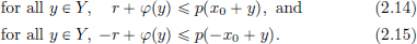
Indeed, once these hold, then multiplication with t > 0 yields

which, in light of the fact that every element from Y can be written in the form ty with y ∈ Y, gives (2.13) with α = ±t ≠ 0. For α = 0, (2.13) is already satisfied according to the hypothesis. Now the inequalities (2.14) and (2.15) are equivalent to the statement:

But there exists such a r precisely if all numbers φ(y) – p(–x₀ + y), with y ∈ Y, lie to the left of all numbers –φ(z) + p(x₀ + z), with z ∈ Y, that is,

that is, if for all y, z ∈ Y, φ(y) + φ(z) p(–x₀ + y) + p(x₀ + z). But this is indeed the case since we have for all y, z ∈ Y that

Now from (2.16) it now follows that:

and it is sufficient to choose, for instance,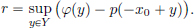

(In general, the sup and the inf here are unequal, and we can choose r arbitrarily from an interval.) Now the number r also satisfies (2.14) and (2.15) and thus from (2.13), we have obtained an extension to Y + (span {x₀}) such that (2.12) holds.

Now the idea is that we extend φ one dimension at a time in order to get an extension to the space X. If X were finite dimensional, then it is clear that this can be done. After dim X – dim Y steps we will have obtained a linear transformation Φ : X → R that satisfies (2.12).

In the general case, the proof goes through, in essentially the same manner, by successive one-dimensional extensions, but we won’t be able to get an extension to X in finitely many steps. In order to complete the process, we will use Zorn’s Lemma.

Zorn’s Lemma

Zorn’s Lemma says that a partially ordered set P with the property that every chain has an upper bound in P possesses a maximal element. The terms are explained below.

A partial order on a set P is a relation on P satisfying

•(transitivity) for all x, y, z ∈ P, x y, y z ⇒ x z,

•(antisymmetry) for all x, y ∈ P, x y, y x ⇒ x = y,

•(reflexivity) for all x ∈ P, x x.

A set with a partial order is called a partially ordered set.

A familiar example is R with the usual relation, but the situation can be much more general: for example, consider R² with the order: (a, b) (c, d) if a c and b d. This latter example justifies the terminology partial. Indeed, is not a total order because not every pair of elements can be compared with : we have neither (0, 1) (1, 0) nor (1, 0) (0, 1).

A subset C of P is said to be bounded above if there exists an element u ∈ P such that x u for all x ∈ C. The element u ∈ P is then called an upper bound of C.

A subset C of P is said to be chain if for all x, y ∈ C, there holds x y or y x. Thus on a chain C, forms a total order since any two elements in C can be compared with . The set R² with the above order is not a chain, since neither (0, 1) (1, 0) nor (1, 0) (0, 1). However, the diagonal {(x, x) : x ∈ R} is a chain.

An element m ∈ P is called maximal if whenever x ∈ P and m x we have that x = m.

Zorn’s Lemma (named after the mathematician Max Zorn) is an axiom in Set Theory. It can be shown that it is equivalent with the Axiom of Choice: for every family A_i, i ∈ I, of nonempty sets A_i, there exists a map I ∋ i → x_i ∈ A_i.

In order to apply Zorn’s Lemma to complete the proof of the Hahn-Banach Lemma, we proceed as follows.

Consider the set P of all pairs (Z, ψ), where Z is a subspace of X with Y ⊂ Z ⊂ X, and ψ : Z → R is a linear transformation extending φ such that ψ(z) p(z) for all z ∈ Z.

We define the partial order on P by defining (Z, ψ) (Z′, ψ′) if Z ⊂ Z′ and ψ = ψ′|_Z. Then every chain in P has an upper bound, as explained below.

If C is a chain in P, then we can construct an upper bound (Z_C, ψ_C) of C as follows: Let Z_C be the union of all subspaces Z, with (Z, ψ) ∈ C and let ψ_C be the common extension of the linear transformations ψ. More precisely, for z ∈ Z_C, there exists a (Z, ψ) ∈ C such that z ∈ Z, and we define ψ_C(z) = ψ(z). This definition of ψ_C(z) is independent of the choice of (Z, ψ). Indeed, if (Z′, ψ′) also belongs to C, and z ∈ Z′, then we have (Z, ψ) (Z′, ψ′) or (Z′, ψ′) (Z, ψ), and so ψ is the restriction of ψ′ or vice versa. In either case, we have ψ(z) = ψ′(z). The map ψ_C : Z_C → R so defined is linear: Indeed, if z, z′ belong to Z_C, then there exists a (Z, ψ) such that z ∈ Z and there exists a (Z′, ψ′) such that z′ ∈ Z′. We have Z ⊂ Z′ or Z′ ⊂ Z. Suppose that Z′ ⊂ Z. Then also z′ ∈ Z so that for α, α′ ∈ R, we have αz + α′z′ ∈ Z ⊂ Z_C, and so it follows that Z_C is subspace of X, and ψ_C(αz + α′z′) = ψ(αz + α′z′) = αψ(z) + α′ψ(z′) = αψ_C(z) + α′ψ_C(z′). Finally, ψ_C satisfies the inequality ψ_C(z) p(z), z ∈ Z_C, since indeed ψ(z) p(z) for all z ∈ Z, for all (Z, ψ) ∈ C. Thus we see that (Z_C, ψ_C) belongs to P and that (Z, ψ) (Z_C, ψ_C) for all (Z, ψ) ∈ C. This completes the proof that every chain in P has an upper bound.

By Zorn’s Lemma, P has a maximal element (Z_∗, Φ). Then Z_∗ = X. Indeed, if Z_∗ X, then there exists an x_∗ ∈ X\Z_∗, and then from the first part of the proof of the Hahn-Banach Lemma, it follows that we can extend Φ to Z_∗ + (span{x_∗}) with the same estimate given by p, contradicting the maximality of (Z_∗,Φ). Thus we have a linear Φ : X → R that extends φ : Y → R, while satisfying the estimate (2.12). This completes the proof of the Hahn-Banach Lemma!

We will now apply this Hahn-Banach Lemma to prove the Hahn-Banach Theorem, first of all in the case when K = R.

Proof. (Of the Hahn-Banach Theorem; real case.)

Let φ : Y → R be a continuous linear transformation. Then we have:

Now we apply the Hahn-Banach Lemma with p(x) := ||φ|| ||x||, x ∈ X. From (2.17), we certainly have for all y ∈ Y, φ(y) |φ(y)| ||φ|| ||x|| = p(y). Thus, by the Hahn-Banach Lemma, there exists a linear map Φ : X → R, extending φ to X, that moreover satisfies the estimate that for all x ∈ X, Φ(x) p(x) = ||φ|| ||x||. Replacing x by –x, we obtain –Φ(x) ||φ|| ||x||, and so for all x ∈ X, |Φ(x)| ||φ|| ||x||. Hence it follows that Φ is continuous and that ||Φ|| ||φ||. Since φ is the restriction of Φ, we have, on the other hand, also that

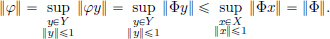
This proves the Hahn-Banach Theorem in the real case.

The proof for complex scalars can be derived from the real case. We remark that real versions of the Hahn-Banach Theorem were first proved independently by Hahn and by Banach. The complex version was given by Bohnenblust and Sobcyzk, following the ideas of Murray.

Proof. (Of the Hahn-Banach Theorem; complex case.)

Let X be a normed space over C. By restricting the multiplication with scalars to real numbers, we obtain a normed space over R, which we denote simply by X_R. If Φ : X → C is a linear transformation, then Φ_R : X_R → R, given by Φ_R(x) = Re(Φ(x)), x ∈ X_R, is also a linear transformation. We now observe below that Φ is completely determined by its “real part” Φ_R. For complex z = a + ib, with a, b ∈ R, we have iz = –b + ia, and hence Im(z) = –Re(iz). So Im(Φ(x)) = –Re(iΦ(x)) = –Re(Φ(ix)) = –Φ_R(ix). Thus

Now if Φ_R : X_R → R is R-linear, then the right-hand side expression of (2.18) determines a C-linear map Φ : X → C:

(1)It is clear that Φ is R-linear.

(2)We have Φ(ix) = Φ_R(ix) – iΦ_R(–x) = i(Φ_R(x) – iΦ_R(ix) = iΦ(x).
Since every complex number is of the form a + ib, with a, b ∈ R, it follows from here and the above part (1) that Φ is also C-linear.

Finally we show that Φ continuous if and only if its real part Φ_R is continuous, and moreover, ||Φ|| = ||Φ_R||.

(1)If Φ is continuous, then since |Φ_R(x)| = |Re(Φ(x))| |Φ(x)| ||Φ|| |x||, we have that Φ_R is continuous and moreover ||Φ_R|| ||Φ||.

(2)Now suppose that Φ_R is continuous and that Φ is given by (2.18). For x ∈ X, let θ ∈ R be such that Φ(x) = e^iθ |Φ(x)|. As |Φ(x)| is real,

so that Φ is continuous, and moreover ||Φ|| ||Φ_R||.

The proof of the Hahn-Banach theorem in the complex case can now be completed as follows. Let φ ∈ CL(Y, C) and let φ_R ∈ CL(Y_R, R) be the real part of φ. Then there exists an extension Φ_R ∈ CL(X_R, R) of φ_R to X_R with ||Φ_R|| = ||φ_R||. Let Φ ∈ CL(X, C) defined by (2.18). Then Φ is an extension of φ, and ||Φ|| = ||Φ_R|| = ||φ_R|| = ||φ||.

Exercise 2.39. (Hamel basis). Let X be a vector space over any field F. Show that there exists a subset B ⊂ X such that B is linearly independent, and span B = X. Such a set is called a Hamel basis of X.

Exercise 2.40. Let X, Y be vector spaces over a field F. Show that any function f : B → Y defined on a Hamel basis B of X can be extended to a linear transformation F : X → Y, that is, F |_B = f. Hint: Every vector in X can be uniquely expressed as a linear combination of vectors from B.

Exercise 2.41. Let X be an infinite dimensional normed space, and let Y be a nontrivial normed space. Prove that there exists a linear transformation from X to Y which is not continuous.

Exercise 2.42. R is a vector space over Q, and hence has a Hamel basis B. Prove that B is necessarily uncountable.

Exercise 2.43. (Additive discontinuous F : R → R). Show that there exists a function F : R → R such that for all x, y ∈ R, F(x + y) = F(x) + F(y), but F is not continuous on R.

Exercise 2.44. (∗)(Banach limits).

Consider the subspace c of ℓ^∞ comprising convergent sequences.

Let l : c → K be the limit functional given by

(1)Show that l is an element in the dual space CL(c, K) of c, when c is equipped with the induced norm from ℓ^∞.

Let Y ⊂ ℓ^∞ be given by

(2)Show that Y is a subspace of ℓ^∞.

(3)Prove that for all x ∈ ℓ^∞, x – Sx ∈ Y, where S : ℓ^∞ → ℓ^∞ denotes the left shift operator: S(x₁, x₂, x₃, ···) = (x₂, x₃, x₄, ···), (x_n)_n∈N ∈ ℓ^∞.

(4)Prove that c ⊂ Y.

(5)Show that there exists a L ∈ CL(ℓ^∞, K) such that L|_c = l and LS = L.

This gives a generalisation of the concept of a limit, and the number Lx is called a Banach limit of a (possibly divergent!) sequence x ∈ ℓ^∞.

Hint: First observe that L₀ : Y → K defined by

is an extension of the functional l from c to Y. Now use the Hahn-Banach Theorem to extend L₀ from Y to ℓ^∞.

(6)Find the Banach limit of the divergent sequence ((–1)ⁿ)_n∈N.

Notes

The proof of the Open Mapping Theorem given in §2.5, and the proof of the Hahn-Banach Theorem given in §2.7 are based on [Thomas (1997)].

 

1 This has nothing to do with the null space: ker T_A := {x ∈ L²[0, 1] : T_Ax = 0}, which is also called the kernel of the integral operator.

² In Fourier/Harmonic Analysis, this is sometimes called the Cesáro summation operator.

³ That is, what Δ_ψ, 〈·〉_ψ, etc. mean.

⁴ The “geometric” series in (2) is called the Neumann series, after the German mathematician Carl Neumann, who used it in connection with the Dirichlet problem.

⁵ For the definition/existence of a Hamel basis, see Exercise 2.39, page 115.

⁶ We remark that if we look at the “matrix” corresponding to L, while thinking of vectors in ℓ² as an “infinite columns”, then the action of L is described by

a matrix with all diagonal entries equal to 0, and with 1s along an “upper” diagonal. So in this case, our “matricial intuition” would have led us astray, since based on the above matrix, reminiscent of a Jordan block in finite dimensional linear algebra, one would be tempted to hastily guess that L has the only eigenvalue 0!

⁷ The usual proof of this is by using some tools from complex analysis. We will instead follow the proof from [Singh (2006)] relying on real analysis techniques.

⁸ See for example [Taylor and Lay (1980), page 287, Theorem 3.2].

⁹ See for example [Taylor and Lay (1980), page 279, Theorem 3.4].

¹⁰ By an unbounded operator, we mean a linear transformation that is not continuous.

¹¹ Named after the mathematicians Hans Hahn and Stefan Banach.