12.1 INTRODUCTION
The role of probability in science and engineering is rapidly increasing, not only in areas of applications but also in the very foundations, such as in quantum mechanics. It is essential that you master this way of thinking. To do so, you need to first learn the language of probability.
Probability has a long and confused history. People generally have an intuitive idea of what probability is, but in practice they often hold contradictory ideas at the same time; and certainly they are often confused about the logical relationship between the probability of an event occurring on a single trial and its frequency of occurrence in a sequence of many trials. To correct some of these logical confusions, it is necessary to start from the simplest elements of the subject.
In this chapter we will examine simple, discrete situations involving probability, and in the next chapter we will examine continuous situations, which are generally the more useful ones in science and engineering. The theory of probability arose mainly from gambling situations, which are typically discrete events such as the toss of a coin, the roll of a die (singular of dice), the draw of a card, or the turn of a roulette wheel, and they still provide the best intuitive approach to the subject. But, as noted, there are often confusions in the mind of the beginner, so please be patient with the following rather pedantic approach to the subject.
We begin with the concept of the toss of a “well-balanced coin,” the roll of a “perfect die,” or the draw of a card from a “well-shuffled deck” (each is clearly an idealization of a common situation in the real world). Consider, for example, the toss of a coin. Each toss is called a trial, and the trials are supposed to occur under identical conditions. We do not mean exactly identical, but rather under conditions that merely seem to us to be identical so far as the coin toss is concerned. Absolute identity in space and time is not possible. The identical trials produce the outcomes that we regard as random. By “random” we mean, at the moment, merely “unpredictable.” We cannot say which of the two outcomes, heads or tails, will occur on any particular trial (toss). We are further assuming that there is no wear and tear on the coin during the repeated tosses, and that each trial is equivalent to any other trial, although the outcomes may be different.
The first thing we do is make a list of the possible elementary outcomes of a trial. Each possible outcome we regard as a point in a sample space (a common mathematical approach to a set of items). Thus we have a space of outcomes (events) corresponding to a trial. In simple problems, like those above, there are a finite number of possible outcomes in the sample space of outcomes. For a coin, the outcomes are H and T; for a die, the outcomes (the top face) are 1, 2, 3, 4, 5, 6; for the draw of a card from a deck (using the standard deck of spades, hearts, diamonds, and clubs), 1S, 2S, … , 13C. An event may involve a number of the elementary outcomes. For example, consider the event that the outcome of the roll of a die is an odd number on the upper face of the die, a member of the set {1, 3, 5}.
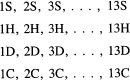
Sample spaces of events are often presented in terms of set theory and Venn diagrams (Figure 12.2-1). Set theory has been taught until the typical student is weary of it, so we will assume that it is familiar. Venn diagrams are apt to be misleading to the unwary. You would probably lay out the sample space of a random draw of a card from a deck in four rows of 13 items each:
The set of odd spades {1S, 3S, 5S, 7S, 9S, 11S, 13S} is scattered and not in one nice connected piece.
We would like to define an elementary event exactly, but recall that the Greeks thought that the world might be made of indecomposable units called atoms, as did science for a long time. Later it was thought that the atoms were composed only of electrons and protons. Still later, further divisions of the elementary particles were assumed. Regularly, what the best minds of one generation considered as elementary later was found to be composed of smaller elements. Yet we need the concept of an elementary event. We “feel” that the individual cards drawn from a deck are elementary units that cannot be further decomposed. However. we must leave the definition of an elementary event as an intuitive concept.
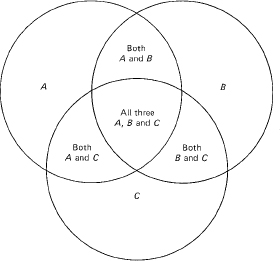
Figure 12.2-1 A Venn Diagram
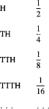
The above examples were sample spaces consisting of a finite number of elementary events. But if the trial is a sequence of tosses of a coin until a head appears. then we have the sample space of possible outcomes (events)
![]()
This sample space of outcomes (n tails followed by a head) is infinite. (T)nH, for all nonnegative integers n.
Students are sometimes bothered by questions like, “What happens if the coin lands on its edge?” or “What happens if the trial is not completed because the coin is lost?” The answers are simple; we do not regard them as possible outcomes (events) of the trials. It is customary to consider only heads (H) and tails (T) as the two possible outcomes of a toss of a coin. Similarly. the roll of a die has six possible outcomes, and the draw of a card has 52 possible outcomes. We simply do not, generally, consider the outcome that a person dropped dead before the trial was completed. We only consider a selected list of outcomes from the class of all theoretically conceivable outcomes of a trial.
Next, we face the problem of assigning a probability to each outcome (event). The founders of probability theory spoke of “equally likely events” and said that the probability of a compound event, such as the face of the die being either 1 or 2, was the ratio of the total number of favorable elementary outcomes to the total of all possible elementary outcomes. For example, the probability of drawing a spade from a deck of cards is the ratio of
![]()
The probability of a 1 or a 2 on the die is the ratio
![]()
The founders of probability theory regarded each possible outcome (event) of the trial of drawing a card from a well-shuffled deck as being equally likely. Similarly, they regarded each outcome of a roll of a perfect die as equally likely. There was confusion when they began to think about compound events like the sequence of tosses until an H appears. Each event in the sample space is not equally likely; only H and T are assumed to be equally likely on a single toss. This kind of distinction is not easy for the beginner to grasp. In this approach to probability it is necessary to decide which are the equally likely events and which are not equally likely events.
The definition of the probability (for the outcomes of the equally likely events) is the ratio of the successes to the total number of possible outcomes. If the given set of outcomes (compound events or simple events) exhausts (but does not duplicate) all possible events of the list of possible outcomes, then the total probability of all these outcomes must be exactly equal to 1. Thus the probability of any particular event is a real number between 0 and 1.
But what is the meaning of “equally likely” if not the assertion of a probability? There is a circularity in the very definition. Probability is an intuitive idea and cannot be based on other than a somewhat circular definition. Therefore, we will examine a bit more carefully why they chose equally likely events as the basic element of the theory.
The toss of a well-balanced coin seems to have equally likely outcomes (what else does “well balanced” mean?). The basic rule of avoiding contradictions in mathematics (and in science generally) requires that we assign the same weight (probability) to things (events) that we find indistinguishable (except for the label H or T, which we assume has no effect on the outcome of the trial). If we did not assign the same probability to each, then we would face the situation that we could interchange the indistinguishable outcomes and thus find different probabilities for the same outcomes of the same trial.
Thus the fundamental tool in assigning probabilities is the basic symmetry of situations, physical, geometric, logical, or algebraic symmetry. Just as congruent figures have the same area, so too in probability theory symmetric situations must have the same probability. Otherwise, we face a logical contradiction.
Unfortunately, experience in physics has shown that sometimes our intuition can be wrong, and that nonintuitive equally likely events are at the basis of the world (as we now understand it).
Applying this symmetry rule to a well-balanced coin, the two possible outcomes are equivalent; hence each outcome must have the probability of ![]() (since the total probability is 1). For a perfect die, each outcome must have the probability of
(since the total probability is 1). For a perfect die, each outcome must have the probability of ![]() , and for the well-shuffled deck, each card has the probability of being drawn of
, and for the well-shuffled deck, each card has the probability of being drawn of ![]() . The words “well balanced,” “perfect,” and “well shuffled” mean that the possible outcomes are all equivalent, and hence have the same probability. Thus in a symmetric situation the probability of each simple outcome is 1/(total number of possible simple outcomes).
. The words “well balanced,” “perfect,” and “well shuffled” mean that the possible outcomes are all equivalent, and hence have the same probability. Thus in a symmetric situation the probability of each simple outcome is 1/(total number of possible simple outcomes).
Probabilities are sometimes stated in the form of odds. For equally likely events the odds of “three to two” implies that the ratio of successes to the total number is ![]() , and the unfavorable ratio is
, and the unfavorable ratio is ![]() . The odds of 1 to the
. The odds of 1 to the ![]() is less easy to explain!
is less easy to explain!
There is often a basic confusion in the student’s mind. We are saying that the mathematically conceived events are equally likely; we are not asserting that the actual physical coins have, or have not, this property. We are modeling reality with the mathematics, but we are not handling reality itself. Common observation shows that a typical coin has something like a 50–50 chance (probability of ![]() ) of being either an H or a T. But a carefully performed experiment using a real coin would probably show some bias, a slight lack of exactly
) of being either an H or a T. But a carefully performed experiment using a real coin would probably show some bias, a slight lack of exactly ![]() for the ratio of the outcomes. We are clearly applying, in this experiment, the concept that probability somehow determines the ratio of the outcomes of many trials. This is not part of the basic definition of probability. One of the main things we must at least partially justify is this connection, which is in your mind. With respect to the conventional die, the very fact that one face has 6 hollowed out spots and the opposite side has only 1 suggests that the center of gravity is not exactly in the middle of the die, and that we will, from this lack of symmetry, find a lack of symmetry in the corresponding outcome frequencies from many trials. But the bias is so slight in practice that the mathematically perfect die does closely approximate the behavior of a real die.
for the ratio of the outcomes. We are clearly applying, in this experiment, the concept that probability somehow determines the ratio of the outcomes of many trials. This is not part of the basic definition of probability. One of the main things we must at least partially justify is this connection, which is in your mind. With respect to the conventional die, the very fact that one face has 6 hollowed out spots and the opposite side has only 1 suggests that the center of gravity is not exactly in the middle of the die, and that we will, from this lack of symmetry, find a lack of symmetry in the corresponding outcome frequencies from many trials. But the bias is so slight in practice that the mathematically perfect die does closely approximate the behavior of a real die.
To repeat the main point, we are modelling reality, we are assigning mathematical probabilities to the outcomes in the list of possible outcomes of a single trial. The relationship between the mathematical model and the actual situation is subject to investigation, but lies outside the theory. In modem physical theory, such as quantum mechanics, there is an increasing acceptance that we can never know, even in principle, exactly what something is, that we must settle for probable values. (Note: It is fashionable in some circles to assert that if in principle we cannot know something then it does not exist!)
12.3 INDEPENDENT AND COMPOUND EVENTS
The concept of independent events is also an intuitive idea. We feel that, in the combined trial of a toss of a coin and the roll of a die, the outcome of the roll of the die is independent of the outcome of the toss of the coin. Actually, we are simply asserting that in the mathematical model they are independent, that the outcome of the coin toss does not influence the outcome of the roll of the die. Therefore, the possible outcomes (events) can be listed as
![]()
There are 12 possible events, and due to the apparent symmetry each should have the same probability of ![]() If the two events, the outcomes of the roll of the die and the toss of the coin, are taken as being independent, then we see that the probability of any combined outcome is the product of the probabilities of its individual outcomes. This is a general rule: for independent events, the probability of the compound event is the product of the probabilities of the simple events. In the above case, we have
If the two events, the outcomes of the roll of the die and the toss of the coin, are taken as being independent, then we see that the probability of any combined outcome is the product of the probabilities of its individual outcomes. This is a general rule: for independent events, the probability of the compound event is the product of the probabilities of the simple events. In the above case, we have
![]()
This follows from the feeling that the list of the 12 events of the trial are all equally likely since the outcomes of the individual parts are equally likely. We do not prove that the two events are independent; rather we assume that they are because we can see no immediate interconnection between them.
This sample space of events is often called the product space. The space of possible events consists of all possible products, one factor from each of the basic sample spaces H, T and 1, 2, … , 6. Note that the corresponding probabilities assigned to the events are the corresponding products of the probabilities of the individual independent events.
But some events are not independent. If we draw a card at random from a deck and return it, shuffle, and then draw again, we feel that the two drawings are independent events. For example, drawing a 4H and a 7S (H = hearts, S = spades) on the two independent draws would be realized by either (“&” means followed by)
4H & 7S or 7S & 4H
since the order of drawing them is supposed not to matter. In this case we have, for each order of the two drawn cards,
![]()
so the total probability of this event is
![]()
On the other hand, if we do not replace the first card before drawing the second card from the deck, then the second drawing is from a deck of 51 cards. The probability of 4H & 7S is
![]()
and is the same as for 7S & 4H. The total probability of the compound event of drawing two cards without replacement is therefore
![]()
which is not the same as when the card is replaced. Why the difference? We easily see that one of the possible outcomes of the replacement trial is that the same card is drawn both times, while in the nonreplacement case this is impossible (p = 0). Thus the ratio of the successes to the total number of equally likely outcomes is different in the two cases; in the second case there are fewer possible equally likely outcomes than in the first case
The probabilities of compound events are based on the probabilities of the simple (elementary) events. The probability of HH in the toss of a coin (assuming independent tosses) is the product of the probabilities of the individual events. The sample space of events is
This is merely the product space (for independent events) H = ![]() T =
T = ![]() taken two times. Note that the compound event of an H and T in either order is
taken two times. Note that the compound event of an H and T in either order is ![]()
It is the general rule (in the mathematical model) that probabilities of independent events are to be multiplied to get the probability of both events happening. This is what we mean by a product space of independent events. If the events in the original spaces are all equally likely, then the events in the product space of independent events are also equally likely
Example 12.3-1
What is the probability of exactly three heads in four independent tosses of a coin? The sample space consists of any sequence of H and T, and each sequence of the four has the same probability (because we are assuming the independence of the tosses). The probabilities of these 24 simple events are each
![]()
This is the probability of each event in the basic sample space of events where each event is the result of four tosses (or four coins tossed at the same time, since both lead to the same product space). How many ways can three heads occur in the four positions, the other position being filled wtih a T? We first list all 16 equally likely possible outcomes of four tosses:
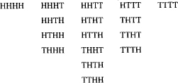
We have put in the first column all heads, in the second column those events with 1 T, in the third those with 2 T's, in the fourth those with 3 T's, and in the fifth column those with 4 T's. We see (from the complete listing) that there are exactly 4 successes out of the total 16 possible outcomes. The ratio gives the probability
![]()
There is an alternative approach to the problem. We note that the probability of getting one of the two faces of the coin is exactly ![]() . The four tosses are supposed to be independent, so the probability of any given sequence is the product
. The four tosses are supposed to be independent, so the probability of any given sequence is the product
![]()
Furthermore, there are only four ways of getting one T (3 H's):
THHH HTHH HHTH HHHT
And each being of probability ![]() , we get
, we get
![]()
as the probability of three H's.
Example 12.3-2
We now consider the trial of a coin toss until a head appears. We regard each single toss as independent of any other preceding or succeeding toss. Each toss has probability of ![]() to be either an H or a T. The compound events, which make up the events of our sample space of runs of tosses until a head, have the corresponding probabilities
to be either an H or a T. The compound events, which make up the events of our sample space of runs of tosses until a head, have the corresponding probabilities
In general we have
![]()
for all n = 0, 1, 2, ….
Do all these probabilities total up to exactly 1 as they should? We have an infinite geometric progression with
![]()
so the sum is [Equation (7.2-3)] the total probability
![]()
The expectation of a variable is defined to be the average over the sample space of the variable you are examining. Thus the expected length of run is the weighted average of the run lengths; each run length is weighted by the corresponding probability of the occurrence of that run length. This is not, as you may think, the average over repeated trials. You think that the two are the same (one average is over the probability space and one is from the average of a long sequence of trials), but we have not proved in what sense these can be the same. You associate probability with long-term ratios of successes to total trials, but that is not how we started to define probability. We got the basic probabilities from symmetry, not from ratios of repeated trials.
The concept of expectation as an average over the sample space is indeed what you “expect” from repeated trials, but you need to be careful. There are traps awaiting the careless person. For example, if you call a head 1 and a tail 0, then the expected value of a single trial is
![]()
which is not any single outcome. You may “expect” to get ![]() from the toss of a coin, but in fact you must get either a 0 or a 1. Similarly, for the toss of n coins (or n tosses of a single coin) you expect n/2 heads, but if n is odd, this is impossible; and in any case you may, due to chance fluctuations, get values far from n/2.
from the toss of a coin, but in fact you must get either a 0 or a 1. Similarly, for the toss of n coins (or n tosses of a single coin) you expect n/2 heads, but if n is odd, this is impossible; and in any case you may, due to chance fluctuations, get values far from n/2.
Example 12.3-3
(Previous example continued) What is the expected number of tosses of a coin before an H appears? If we say that the event H has length 1, the event TH has length 2, and so on then to get the expected length of run until the first H turns up we have to sum the lengths multiplied by their corresponding probabilities; that is
![]()
How can we sum this? Equation (9.10-2) was something like it. Let us look at it. Example 9.10-2 showed that
![]()
If we multiply this identity through by x,
![]()
and then set x = ![]() , we would have our result. Therefore, the
, we would have our result. Therefore, the
![]()
This seems like a reasonable result. (You can always approximately test it by tossing a coin and finding that the average number of tosses needed is approximately two.) If you are dubious about handling infinite series in this formal way, then you can take a finite segment of the geometric series, compute the answer, and then let the number of terms in the series approach infinity.
From these simple examples, we see the need for more elaborate mathematics to count the possible outcomes to be listed in the event space (suppose you asked for 3 H's out of 10 tosses; then you would have a space of 1024 outcomes, which would be unpleasant to list in all detail). We also see the necessity for taking a closer look at the use of the calculus in generating identities from known identities. We now turn to the first of these, after looking at one final example.
Example 12.3-4
There is a famous puzzle based on two coins in two drawers of a box. The problem is that there is a box with two drawers. In one drawer there are two gold coins and in the other drawer there is a gold and a silver coin. Given that you opened at random one drawer, picked at random one coin in that drawer, and you found that it was gold, what is the probability that the other is silver? The false reasoning is that the other coin is either a gold or a silver coin and therefore each has probability ![]() . The correct reasoning goes as follows. The words “at random” mean that both the drawer and the coin have equal probabilities (remember the words “at random”)
. The correct reasoning goes as follows. The words “at random” mean that both the drawer and the coin have equal probabilities (remember the words “at random”)
![]()
The actual trial that found the gold coin eliminated the fourth possibility; there are only three possible outcomes left and each has the same probability, now ![]() (since the sum must be 1). Of these three equally likely outcomes, only one is successful (given that you have already seen the gold coin), and the probability is therefore
(since the sum must be 1). Of these three equally likely outcomes, only one is successful (given that you have already seen the gold coin), and the probability is therefore ![]() . This shows the necessity of watching what are the actual equally likely cases, and the advantage of imagining an experiment that might be done to test out the result. This is an example of conditional probability (see Section 12.9); the probability is conditioned having found a gold coin in the first drawer.
. This shows the necessity of watching what are the actual equally likely cases, and the advantage of imagining an experiment that might be done to test out the result. This is an example of conditional probability (see Section 12.9); the probability is conditioned having found a gold coin in the first drawer.
12.4 PERMUTATIONS
There is a simple rule for combining independent choices. If the first selection can be made in n1 ways, the second independent choice in n2 ways, and the third independent choice in n3 ways, then the number of ways you can choose a set consisting of one from each is
N = n1n2n3
This rule (generalized in an obvious way, which we need not state) is very useful in solving problems involving the selection of items. It is simply the product space of the individual independent sample spaces (choices).
Example 12.4-1
Suppose we have four items, and label them A, B, C, and D. In how many ways can we arrange them? We make a systematic list.
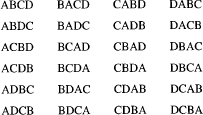
There are 24 cases. We may analyze them in the following way. The first letter could be picked in any of four ways (the four columns). The second letter could be picked in any of three ways, and finally the third letter could be picked in any of two ways; the last letter is forced to be the one left over. Thus we have the product
4 × 3 × 2 × 1 = 24
as the number of ways of selecting the four items.
Suppose we have a collection of n distinct items. In how many ways can we arrange them when we regard different orderings as being different? Evidently, we can choose the first item in any of n ways, the second item as one of the n – 1 remaining items, the next item from one of the n – 2 items, and so on, down to the last item, which is the one that is left. As we think about it, we see that there will be a total of
n(n – 1)(n – 2) … (2)1 = n!
distinct ways of selecting the n items. These are called permutations, because if we permute (interchange) items we have distinct selections. In mathematical notation we have
P(n, n) = n!
Rule: The number of permutations of n things taken n at a time is n!.
Example 12.4-3
Suppose from the same four items A, B, C, and D we select only two items (independently). We can get
AB, BA, AC, CA, AD, DA, BC, CB, BD, DB, CD, DC
which are 12 arrangements (permutations). We could reason as follows; the first letter could be picked in any of four ways, and the second letter in any of three ways, which makes a total of
4 × 3 = 12
ways.
Generalization 12.4-4
If, from a collection of n distinct things, we select only r of them, then we have
P(n, r) = n(n – 1)(n – 2) … (n – r + 1)
different permutations since we can select the first in n ways, the second in n – 1 ways, the third in n – 2 ways, on down to the rth, which is selected from the n – r + 1 things that are left at that time. If we multiply both numerator and denominator by (n – r)!, we get
![]()
which is the number of permutations of n things taken r at a time. Rule: The number of permutations of n things taken r at a time is n factorial divided by n – r factorial.
Example 12.4-5
The birthday problem. We wish to know the probability that one or more persons in a room will have the same birthday. It is natural to assume that the individuals have birthdays that are independent (that both of a known pair of twins, for example, are not there at the same time), that birthdays are uniformly probable over all the days (which is slightly wrong), and that there are exactly 365 days in a year (which is definitely wrong by a very small amount). The errors in the assumptions are all fairly small.
We begin by inverting the problem (a very common thing in probability) and compute the probability that no two persons have the same birthdate. We can do this in one of two ways. If we ask, “How many ways can we select the k people, one at a time, from the 365 days with no duplicates?” the answer is that this is the number of permutations of n things taken k at a time:
P(365, k)
This is the number of successes. Next, how many sets of k (with duplicates) can you select? This is
365k
and is the total number of equally likely elements in the sample space. The ratio of successes to the total possible is the desired probability
![]()
The second approach is to deal in the probabilities from the start. We can select the first person with probability (of a duplicate birthday) 365/365 = 1 of success, the next with probability 364/365, the next with probability 363/365, … , and the kth with probability (365 – k + l)/365. Reasoning that these are independent choices, then the probability that no two persons have the same birthdate is the product
![]()
What was asked for was the probability P (k) = 1 – Q (k) of a duplicate, which is
![]()
It surprises many people that when k = 23 the probability P (k) is greater than 1/2. We give a short table to show how P (k) depends on k.
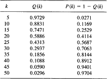
A pair of interesting numbers are P(22) = 0.4757 and P(23) = 0.5073. With 23 people in a room (and the assumed independence), there is better than a 50% chance of a duplicate birthday.
Why is this true? You tend to forget that with k people there are k(k – l)/2 possible pairs to have duplicate birthdays; you tend to think of yourself having a birthday in common with someone else, forgetting that this also applies to everyone else in the room.
Example 12.4-6
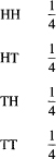
Biased coin. How can you get an unbiased choice from a coin that is biased? Simple! If you toss the coin twice, you have the sample space with the probabilities (where p = probability of an H and q = 1 – p)
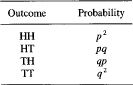
We notice that HT and TH have the same probabilities. Thus we call one outcome (say HT) the event H and the other outcome (say TH) the event T, and if either of the other two cases occurs, we simply try again. We can get an unbiased decision from a biased source.
It is interesting to compute the expected number of double tosses to get a decision. You get a decision with probability P = 2pq, and you fail to get a decision with probability Q = 1 – P. Thus you have the equation (one trial = a double toss)
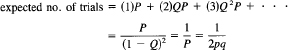
If the coin is unbiased, p = ![]() , you can expect two (double) tosses, but the more biased the coin is, the longer you will have to toss until you get a decision.
, you can expect two (double) tosses, but the more biased the coin is, the longer you will have to toss until you get a decision.
1. In how many ways can you select seven items from a list of ten items?
2. In how many ways can you go to work if you have a choice of two cars, four routes, and seven parking spaces?
3. In how many ways can you select (independently) a shirt, jacket and shoes if you have nine shirts, three jackets, and four pairs of shoes?
4. What is the probability that two faces are the same when you roll two dice?
5. What is the probability of a total of 7 on the faces of two dice thrown at random?
6. What is the probability of each sum on the faces of two dice?
7. Assuming that each month has 30 days, what is the probability of two people having the same birthdate (in the month) when there are k people in the room? Where is the 50% chance point?
8. If I put k marbles in ten boxes, what is the probability of no box having more than one marble?
9. Write out all the permutations of two items selected from a set of five items.
10. If the amount of change in a pocket is assumed to be uniformly distributed from 0 to 99 cents, how many people must be in a room until it is at least a 50% chance that two will have the same amount of change?
11. How many three-letter arrangements can you make of the form consonant, vowel (a, e, i, o, u), consonant?
12. Criticize the proposal that 50 people use the last three digits of their home phone number as a private key for security purposes with the requirement that no two have the same key.
12.5 COMBINATIONS
Frequently, the order in which the numbers from the selected set occur is of no importance. Thus, when dealing cards in a card game, the order in which you receive the cards is often of no importance. When order is neglected, the sets are called combinations.
If we start with the number of permutations P (n, r), how many of them are the same when we ignore the order? There are exactly r\ orderings of r things, so r! different permutations all go into the same combination. Thus the number of combinations of n things taken r at a time is
![]()
These are exactly the binomial coefficients of Section 2.4. (We saw them in the table of heads and tails in Example 12.3-1; the number of items in the columns were 1, 4, 6, 4, 1.) Therefore, we are justified in using the same notation for the quite different appearing things; they are the same numbers. You see the central role that the binomial coefficients play in the theory of combinations. This is an illustration of the fact that mathematical functions devised for one purpose often have applications to very different situations, the universality of mathematics (Section 1.3).
Example 12.5-1
This observation supplies an alternative proof of the binomial theorem (Section 2.4). We consider
![]()
Let us multiply out the first stage (keeping the order of the factors)
(a + b)a + (a + b)b = aa + ba + ab + bb
The next stage gives
aaa + baa + aba + bba + aab + bab + abb + bbb
At the nth stage, the number of times we will have
akbn – k
is the number of ways a can occur in k places of the n possible places. This is C(n, k) times. Thus it will give rise, when these terms are all combined, to the term
C(n, k)akbn – k
The whole expansion will be
![]()
which is the binomial theorem. Thus we have given a “counting” proof of the binomial theorem in place of the earlier inductive proof.
This also means that what we learn in one of the situations can be applied to the other. For example, we showed that
C(n, r) = C(n, n – r)
In the new situation, this says that the number of combinations of n things taken r at a time is the same as the number of combinations of n things taken n – r at a time. The truth of this is seen when you count the combinations of those that are not taken; they match, one by one, those that are taken. What you take is uniquely defined by what you leave.
Another example of this transfer of knowledge is the binomial identity
C(n, 0) + C(n, 1) + C(n, 2) + … + C(n, n) = 2n
which is the same statement we proved in Example 2.3-4 of counting the number of subsets (proper and improper) of a set of n items.
Example 12.5-2
How many different hands of 13 cards are possible? There are conventionally 52 cards in a deck, and in a hand of cards the order of the cards is of no importance; so we have
![]()
which is a very large number. We will leave to later how to estimate such numbers. We note, however, that it can be written as
![]()
which is fairly easy to compute on a hand calculator.
1. In two independent draws of a card from a deck, what is the probability of getting a duplicate?
2. How many different bridge deals can be made, regarding the various positions as independent?
3. What is the ratio of the number of combinations to the number of permutations of n things taken A: at a time?
4. How many sets of k items can be selected from n items?
5. How many hands of seven cards are possible?
6. How many teams of 5 players can be selected from a class of 20 students?
7. What is the probability of seeing 7 heads in the toss of 12 coins?
8. Given n items, show that the number of combinations involving an odd number of selected items equals the number of combinations in which an even number are selected. Hint: (1 – 1)n
9. What is the probability P (k) of a run of length k for rolling a die until a duplicate number apperas?
12.6 DISTRIBUTIONS
Example 12.6-1
Now that we have the mathematical tools and notation, we are ready to explore questions such as the number of possible outcomes, say, of ten tosses of a (mathematical) coin. There are
210 = 1024
possible outcomes. How many have 0, 1,2,…, 10 heads? These are simply the numbers
C(10, k) (k = 0, 1, … , 10)
These eleven numbers give the distribution of the number of heads that can occur in ten tosses of a coin (see Figure 12.6-1). They can be computed sequentially using the rule of Section 2.4. They are
1, 10, 45, 120, 210, 252, 210, 120, 45, 10, 1
which add up to the required 1024 cases in total. Each of the 1024 events is equally likely, provided both the original individual H and T were equally likely and the tosses were independent. Therefore, to get the probabilities, we merely divide the above numbers by the total number of equally likely possible outcomes. Thus the probability of k heads is
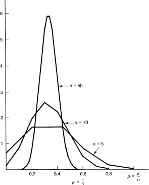
Figure 12.6-1
Prob{of exactly k heads in ten trials} = ![]()
This is the distribution of the probability of k heads in ten trials and the total probability is 1. The sum of all the probabilities is 1 since the sum of the binomial coefficients of order n is 2n.
Suppose we have a binary event (a trial with only two possible outcomes) and one of the outcomes has probability p. The other outcome naturally has probability 1 – p. Conventionally, we write
![]()
as the complementary probability to p. Let a “success” have probability p; then the “failure” has probability q. For example, items coming down a production line may be “good” or “bad.” A medical bandage may be sterile or not. A single trial may succeed or fail. When interviewing people, a single trial (asking a person a question) may yield a response or no response. In an experiment, a mouse may or may not catch a disease. These yes-no situations in which the trials are independent are very common in life, and are called Bernoulli trials, since Jacques (James) Bernoulli (1654–1705) first investigated the theory extensively.
Example 12.6-2
For n Bernoulli trials, what is the distribution of the possible outcomes? There are n + 1 possible outcomes if we ignore the order in which the events occur. In how many ways can exactly k successes occur? There are C(n, k) ways of this happening. Next, what is the probability of each of these individual events? The probability of exactly k successes followed by n – k failures must be
pk(1 – p)n – k
This is the probability for any preassigned sequence of k successes and n – k failures Thus the distribution of the probability of k successes is given by the function
![]()
which is the number of different ways it can occur times the probability of the single event. In Figure 12.6-1, there is a plot of this for p = ![]() and for both n = 5 and n = 10. In both cases the total probability is, of course, exactly 1. This can be verified mathematically, because they are the individual terms obtained by expanding the binomial
and for both n = 5 and n = 10. In both cases the total probability is, of course, exactly 1. This can be verified mathematically, because they are the individual terms obtained by expanding the binomial
(p + q)n = 1
remembering that p + q = 1. Note: This result (12.6-2) agrees with the result of Example 12.6-1 when p = ![]() .
.
Example 12.6-3
Frequency of occurrence in Bernoulli trials. We can now make a connection between the probability p of a success in a single trial and the probability P (k) of k successes in n independent trials. By (12.6-2), the probability distribution function for k successes is
P(k) = C(n, k)pk qn – k
For what value(s) of k is this a maximum? This is a discrete maximization problem We write
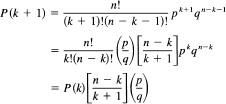
The function P (k) is increasing when
![]()
If the equality holds, then there are two terms of the maximum size.
Thus we see that the distribution function P (k) for k successes in n trials (derived from the product space of single trials) rises for values k < np – q and falls for values k > np – q. Figure 12.6-1 and a little familarity with the binomial coefficients show the increasing peakedness of the distribution function P (k) as n gets large. The peak is near p = k/n. The number of successes divided by the total number of trials is near p.
Distributions of many other kinds of events can be computed. The above distributions are simply a grouping of the original terms that had the same probabilities into a single term. This term is exactly k successes out of the n trials; that is why the number of times something can occur is so often needed.
Given a distribution, it is common to ask, “What is the expected value of this distribution?” (Section 12.3). This is the same thing as the average over the sample space. The average of what? Of the number of successes, presumably. Thus we are asked to compute the expression (the expected value)
![]()
where k is the number of successes. The notation requires some explanation. The letter k is the dummy index of summation and could be changed to any other letter we pleased. But we have the letter K on the left-hand side. What is the meaning of K1 It gives a clue, via the variable of summation, to what is being computed. It is k times the probability of k successes that goes into the sum. If we had written
E{K2}
this would mean
![]()
the sum of the square of k multiplied by the corresponding probability from the distribution we are averaging over.
Example 12.6-4
To find a more compact form for representing the expected value (12.6-3),
![]()
we have to think how we can create the appropriate identity. The C(n, k) come from the generating function (2.4-1):
(1 + t)n
Looking at our expression (12.6-3), we finally think that starting with
would be a good idea since it looks something like what we want. We have
![]()
If we differentiate this identity with respect to t, we will have the correct coefficient in front of each binomial coefficient. We now set t = 1:
![]()
The difference in the ranges of summation between this and the one we started with (which began with 0) has no effect since the omitted term is multiplied by 0. Now, using the fact that p + q = 1, we have, finally,
![]()
In words, the expected value of the binomial distribution is the number of trials times the probability of a success.
We regard E{ } as the expectation operator (just as we regarded d{ }/dx and ∫ … dx as operators), operating on a function to be supplied in the braces. The expectation is a linear operator. The function operated on is to be multiplied by the corresponding probability of occurring and then summed over all possiblecases that can occur. The denominator of the averaging is the sum of the probabilities, and, since this is always 1, it can be ignored.
We have the simple rules (A and B are constants)
![]()
When computing an average (expected value), it is important to ask, “Whose average?” The following example will illustrate this point.
Example 12.6-5
Suppose there is a chemistry department that has
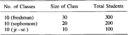
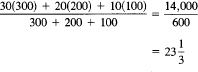
What is the average class size? If you ask the faculty, they will say that the average class size is 20, since
But note that half the students are in a class of size 30. If we ask the average size as seen by the students, we get
Now suppose that the chemistry department decides to combine the 10 freshman classes into one large lecture, and then use the 9 free lecturers to add 9 jr.-sr. courses of size 10 (thus increasing the number of advanced students by 90). You now have:
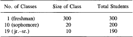
The faculty would now say that the average class size is
![]()
but the students would see the average class size as
Thus you see how different the service offered looks from the point of view of the people offering the service (23) and those getting it (139). This explains the well-known phenomenon that the airlines claim that many flights are fairly empty, but the customers see mainly the crowded flights (after all, no passenger has ever flown on a completely empty flight!). This same phenomenon applies to crowded nursing homes, jails, transportation systems, and so on. Notice how small fluctuations from average as they grow in size are rapidly transformed to very great differences in the quality of service as seen by the customer.
Generalization 12.6-6
Find the general formula for computing the phenomenon in Example 12.6-5. We begin with the distribution n, units of size si. The server computes
![]()
the consumer computes
These are very different things! They are the same only if all the sizes st are the same. Once there is a reasonable variability in the sizes, then rapidly the customer tends to be in the big groups and sees a degradation in the quality of service. Thus there is a simple rule: to improve the quality of the service, you should work hard on the worst cases and not spend a lot of time on the slightly bad cases.
1. Find the maximum in Example 12.6-3 by differencing the successive terms P(k + 1) – P(k).
2. Apply the theory of Generalization 12.6-6 to the class sizes you currently have.
3. Compare the case of three classes, each of size 5, with three with sizes s – k, s, and s + k.
4. What is the expected value of the distribution of the number of rolls of a die until a 6 appears?
5. What is the distribution of the number of double tosses of a biased coin until you get a matching pair? Find the expected value.
12.7 MAXIMUM LIKELIHOOD
In the above probability problems we assumed that we had the initial probabilities. In statistics we invert things, and we start with the results of the observations. Assume that we have made n Bernoulli trials and have seen exactly k successes. What is a reasonable value to assign to p? Of course, any value of p might have given the result of k successes, but some are very unlikely to have done so.
In this situation we need a rule to decide which value of p we should pick from all the possible values of p available. Bernoulli suggested that we take the p that is “most likely.” True, the outcome of the n trials is a random event, and p could be number 0 ≤ p ≤ 1, but what is a reasonable choice for the unknown value of p? Bernoulli argued that in the absence of other information, you should choose the value of p that is “most probable,” most likely to give rise to what you have observed, the one with the maximum likelihood. How could you seriously propose to choose a very unlikely value of p? It is, of course, implied that the distribution of outcomes has a single, sharp peak, and not two or more approximately equal sized peaks. In this latter case, the concept of picking the most likely probability has much less sense. Maximum likelihood applies mainly to single, sharp peak situations.
Example 12.7-1
Find the value of p for the maximum of the function P (k) for k successes in n Bernoulli trials,
To find the value of p, you differentiate and set the derivative equal to zero. In this maximizing process, the leading constant coefficient C(n, k) has no effect, so you can ignore it and maximize, as a function of p, the expression
![]()
The derivative is
![]()
Divide out the common factor pk – 1(1 – p)n – k – 1 to get
![]()
Solve for p:
![]()
This is exactly what you would expect! If all you know is that there were k successes out of n Bernoulli trials, you would guess that the probability is the ratio of the successes to the total number of trials, k/n.
Beware! This is not the probability; it is your “best guess” at it, it is the “most likely value.” Due to the method used, the result must be a rational number, but we saw in Section 3.6 that rational numbers have decimal representations that are periodic, so it is very “unlikely” that the “true” probability is a rational number. It is your estimate that is a rational number. Probabilists deal with given probabilities; statisticians infer likely values for probabilities and do not deal with the certainties of the probabilists. Furthermore, you might have seen a very unlikely set of trial outcomes and be very far from an accurate estimate of p.
But we have done more. We have made another connection between the idea of probability (based on symmetries in the product space of repeated independent trials) and the idea of the frequency of occurrence (based on repeated trials). It is the principle of maximum likelihood which says that what we observe should be the most likely event in the product space of events. It is true that this is only an assumption, but in the one use (so far) of this principle the result agrees with common sense (often meaning uncommon sense!).
One verification does not establish a principle as being infallible. Indeed, no finite number of verifications can do it. Maximum likelihood must remain a very plausible principle, and it is not a mathematically derived result. We will, in Section 13.6, derive a similar result that connects the probability with the frequency of occurrence.
The Bernoulli assumption of maximum likelihood is that you should take the value of the unknown parameter (in this case the value of p) that is “most likely” to give rise to the observations you have seen. It seems hard to argue that you should arbitrarily pick any other value of p, that you should pick an unlikely value—one less likely to give rise to what you have seen—but this is not a proof that the maximum likelihood principle always gives the “best” value for an unknown parameter. It remains a very plausible rule, a very useful rule, but arbitrary in the final analysis.
Example 12.7-2
Proofreading. It is a common experience to have two different people read a table of numbers to find the errors that may be in the table. Suppose the first reader finds n2 errors (wrong digits), the second reader finds n2 errors, and that when the two lists of errors are examined there are n3 errors in common. Can we make any reasonable guess at the remaining errors in the table? Answer: not if we do not make some assumptions about the process of finding the errors. The assumptions we make must be very simple since we lack much data on the subject. A realistic model would require extensive measurements of both the kinds of errors and the habits of the readers. We therefore make a rather idealistic model.
We will assume that there is an unknown number N of errors in the table and that each is as easily found as any other. Second, we will assume that the two readers find errors independently of each other. These are ideal assumptions to be sure, but they are plausible, and they enable us to make a guess at the number N.
From Example 12.7-1, we see that a reasonable assumption for the probability of the first reader finding an error is
![]()
and for the second reader we have correspondingly
![]()
Now what is the probability of both readers finding the same error? Since we assumed independence in the reader’s abilities to find errors, it is
![]()
Eliminate p1 and p2. You get
![]()
and, supposing that n3 is not zero, you have an estimate of the total number N of errors in the table:
![]()
Is this reasonable? We try some extreme cases. If both readers found exactly the same errors, then nx = n2 = n3 = N. This means that all the errors were found and that both readers were perfect, pi = 1. Yes, this is reasonable. At the other extreme, suppose there were no common errors. Then N is infinite! This means that the readers were very bad at finding errors since they found none in common. The result is, in a sense, reasonable, although it is unrealistic since the table must have been finite to begin with (although we made no claim as to the size).
There were many assumptions in getting this formula. First, you are guessing at the values of the pi. Second, the expected number of errors may be a fraction, but the number observed must be an integer. Finally, you are dealing with probabilities, and you may have seen an unlikely example of the readers’ abilities. The above result is thus more understandable.
Another exception to this reasoning occurs if we assume that either reader found no errors. Say n2 = 0. This means, of course, that n3 = 0. If ni is not zero, then we have removed only those errors the first reader found, and we have no real estimate of the original number of errors in the table. If neither reader found any errors, we are inclined to assume that the table is perfect, but it could be that both readers were no good; we simply cannot choose between these two cases without outside information such as the known performance of the readers in other situations.
We have not yet found the answer to the original question, the number of errors left in the table. It is easy to see that
N – n1 – n2 + n3
is a reasonable answer, since the first two subtractions each remove the common errors, and we should add the common errors back to get a reasonable result. Again, we test the formula by common sense. When you go through the exercise, you find that the formula is at least plausible, although certainly not perfect.
This is a good example of the use of probability in common life. The assumptions that must be made to get anywhere (without a large number of measurements) are often somewhat unrealistic, yet the result is a “better than nothing” guide. If we find that the estimated number of errors is larger than we care to tolerate, then we will have to get further readers to search and make further measurements on the common errors between each of the readers. On the other hand, if the estimated number of errors left is quite low, we are inclined to let the table go and concentrate on other things. The case of three readers is much more complex as there will be four unknowns (P1, P2, P3, N) and seven conditions, which suggests a least square approach.
12.8 THE INCLUSION–EXCLUSION PRINCIPLE
If there had been three readers in the above example of proofreading, then we would have had to subtract out the errors found by all three individually, add back those that were found by each pair, and then subtract out again those that were common to all three. This is a special case of the general inclusion-exclusion principle, where we alternately add and subtract the larger and larger commonality. Consider a particular item that is common to m sets. If we add all the times it occurs in a set A,, we will have m = C(m, 1) of them and this is too many. Next we subtract all the times it occurs in two sets Ai, Aj, –C (m, 2), and then add all the times it occurs in three sets AiAjAk, C(m, 3), and so on. As a result we have counted the item
C(m, 1) – C(m, 2) + C(m, 3) – … + (–1)m – 1C(m, m)
But the sum of all the binomial coefficients of order m [we neglected C (m, 0)] with alternating sign is zero since
(1 – l)m = 0
Hence the above sum is exactly 1, and we have finally entered the point a net of 1 time. Thus the above formula gives an alternative way of counting a set.
Example 12.8-1
There is a famous problem in probability that can be phrased in many ways. One way is to imagine n letters and n envelopes addressed separately, and then the letters are put in the envelopes at random. What is the probability that at least one letter will be in the right envelope? Again, if you number a set of items 1 to n, mix them up, and count down from the top, what is the probability that the rth item will occur at the rth count?
To apply the above formula, we first note that the probability that a letter is in its proper envelope is 1/n. We designate the event that the ith letter is in the ith envelope by Ai. There are exactly n such trials (one for each letter i); hence we have for the first term
![]()
For a pair of letters, the probability that the first is in its envelope and that the second is in its is 1 /n(n − 1), and there are C(n, 2) such pairs. This gives the second term
![]()
correspondingly, we have for triples,
![]()
This continues through the n possible terms; and when they are added with alternating sign, we get for the probability that at least one letter is in its correct envelope
![]()
In view of the rapid rate at which the individual terms approach 0, it is evident that for even reasonable sized n the value of pn is close to its limiting value (n = ∞) of 0. 63212 …. By n = 7, the correct value and the limiting value agree to four decimal places. Thus whether there are 10 letters or 10,000, the probability of at least one letter being in its correct envelope is about the same. Correspondingly, the complementary probability that no envelope has its proper letter is 0.36788 … . We will see later (Section 20.8) that the number called e = 2.71828 … is involved in the limit of Pn as rc → oo; that is, Pn −∞ 1 – 1/e.
This is an example of the famous Problème de recontres, or matching problem, whose solution was given by Montmort (1678–1719) in 1708.
1.* Work out the details for a theory for three proofreaders, given the number of errors of each, each set of errors common to two, and the number common to all three.
2. Show that the number of integers ≤ N that are not divisible by the primes 2, 3, 5, and 7 is where [N/i] means (here) greatest integer not greater than N/i, and the sum is over all given primes, all unlike pairs of primes, and so on. If N = 210n, show that this number is 48n.
![]()
3. Suppose n balls are placed at random in m boxes. Let Ai be the event that box i is empty, for i = 1,2, … , m. Show that (a) P(Ai) = (m – 1)n/mn, P(AiAj) = (m – 2)n/mn for i ≠ j, and so on. Hence we have Sk = C(m, k)(m – k)n/mn, where Sk is the sum of all the terms of single, double, and so on, occupancy, (b) Show that the probability of no empty boxes is E(– 1)kC(m, k)(m – k)n/mn.
12.9 CONDITIONAL PROBABILITY
We have seen a couple of examples of situations where the probability was conditional on what happened. There are the original probabilities, often called a priori (prior) probabilities, and then there are the probabilities a posteriori (posterior means after), after some event has happened. For the two drawers and the gold and silver coins (Example 12.3-4) the original distribution of four possible outcomes was equally likely (a priori), but, having seen a gold coin, the distribution was now conditional on that, and one outcome was excluded. Similarly, when we draw a card from a deck, and then draw another card without replacing the first, the probabilities are conditional on what was first drawn. If the first card was a ten of diamonds, then the probability of another ten of diamonds is 0, and the probability of any other named card is 1/51 (not 1/52).
Example 12.9-1
Information. Suppose you draw one card from a deck, do not look at it, and then draw a second card. What is the probability that the second card is 10D? If the first card drawn had been the 10D, then the probability would be zero; but if it had not been the 10D, then the probability would be 1/51. We need to combine these two probabilities with their probability of occurrence, that is, 1/52, and 51/52. Thus using these conditional probabilities we get
![]()
This is the same as if the first card had not been drawn. We learned nothing (got no information) from the first draw, so it is not surprising that the probability was not affected. This is a general principle, if nothing is learned, you can ignore the event; but it is sometimes a subtle question whether you have, or have not, learned anything.
Often, in a sequence of trials, what happens at one stage can affect the later events. This is the concept of conditional probability. We use the notation
![]()
to mean “the probability of x given that y has occurred.” The vertical bar is the condition sign, and what follows is assumed to have already happened (a typical inversion of notation!).
Example 12.9-2
Bayes’ Relationship. There is the original sample space of all possible pairs of events p(x, y). We see that conditional probability is effectively defined by the equation
![]()
In words, the probability of the pair x and y occurring is equal to the probability of y occurring followed by the conditional probability of x given that y has occurred. But supposing we look first at the event x then this can also be written as
![]()
Since these two probabilities are the same, we have
![]()
or, if p(x) ≠ 0,
![]()
This is a special case of the famous Bayes relation. It relates the two conditional probabilities; it is the device that enables you to reverse the arguments in the conditional probabilities. More generally, if y is composed of independent sets yi9 then since
![]()
we get, similarly,
![]()
The equation is above reproach, but there is great controversy over its use.
The failure to recognize such conditional effects can be serious in science, as the following case study shows.
Case Study 12.9-3
ESP. There is a widespread belief that some people have extrasensory perception (ESP), meaning that, for example, they can foretell the random toss of a coin or in some way influence the outcome of the toss of the coin. Among the believers in ESP, there is also the belief that this ability comes and goes, that sometimes you have it and sometimes you do not.
To test the presence of ESP, the following experiment is proposed. We will make ten trials in all. If the first five show that ESP is present, we will go on; but if it is not present, then there is no use wasting time on this test. How shall we decide if it is present or not? If the first five trials show three or more successes, then we will assume that ESP is present and go on; otherwise, we will abort the test.
Let us analyze the experiment from the point of view that there is no such effect as ESP, that calling the correct head or tail is solely a matter of luck.
What is the sample space of the first five trials? There are six possibilities, 0, 1,2, 3, 4, or 5 successes. We have the following table:

The expected number of successes is 5/2. But conditional on achieving at least three correct guesses, the expected value is
![]()
which is about 7/2 rather than 5/2. Thus the conditioning has influenced the expected number of right guesses (as you would expect).
For the second five trials, we expect
![]()
successes. The sum of the two expected values is
![]()
which is very close to 6 (16 x 6 = 96).
Without this optional stopping after the first five trials, the expected number of successes in the ten trials is five. By optional stopping and saying that ESP is not present in the current run of trials (and thus not counting the trials that contained a lot of failures), we have raised the expected number of successes from five to almost six.
If I am allowed to proceed this way, then I can make so many runs that the experiment will appear to show significantly better results than chance, that there is such a thing as ESP. These arguments in no way prove that there is no such thing as ESP, but are designed to alert you to any experiments where there is optional stopping; even in a physics lab sometimes a run is aborted because …. Again, this is not an argument that every run that is started must be completed no matter how obvious it is that an error has occurred; it is a warning to be very careful when you engage in optional stopping. You may find what you set out to find, and not what the experiment was supposed to reveal about the world.
12.10 THE VARIANCE
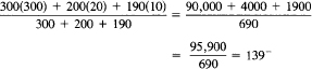
Given a distribution in the random variable k, we have introduced the expectation of k, E{K}, as one measure of what statisticians call “typical values.” Another typical value is the median, which is the value (or average of two adjacent values) for which there are as many items above as there are below. A third typical value is the mode, which is the most fashionable, the most frequently occurring value (if there is one). All these are summarized in Figure 12.10-1.
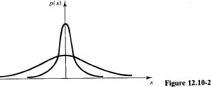
We all know that there is usually a spread about the average (see Figure 12.10-2), that some distributions are centered close to their average value and some are spread out. To measure the spread, we introduce the variance about the mean as the average of the squares of the distance from the mean. In mathematical symbols, using ¡i (Greek lowercase letter mu) as the expected value of the distribution,
μ = expected value of the distribution = E{K}
![]()
then we have for the variance (σ2) (Greek lowercase sigma)
Figure 12.10-2
![]()
where p(k) is the probability of the k occurring.
Example 12.10-1
What is the variance of a Bernoulli distribution? The variance V{K} is defined as the second moment about the mean, and the mean of n Bernoulli trials is μ = np. Thus
![]()
The term (k – np)z can be expanded into three terms (we temporarily drop the range of summation for convenience):

The middle sum we have just done in (12.6-6), and it is simply np. The sum in the last term is obviously equal to 1 (it is the sum of all the probabilities). Thus it combines with the middle term to give, finally,
![]()
To attack this summation term, we proceed along the lines we did to get the average value. We start with the generating function (12.6-5):
![]()
If we (1) differentiate this with respect to t, we will get a coefficient k then if we (2) multiply through by t, we will be back with the same power of t ready to differentiate again; so we (3) differentiate again with respect to t to get a second factor of k; and then (4) set t = 1 to get rid of the generating variable t; and, finally, (5) recall that p + q = 1. We have therefore to compute
Doing steps (1) and (2), we get
![]()
We now differentiate again to get for step (3)
![]()
We now carry out step (4), which requires us to set t = 1. Finally, we do step (5), put p + q = 1, to get the sum we want:
![]()
Now going back to the formula for the variance of the Bernoulli distribution(12.10-4), we have
![]()
This is a very nice, compact formula for the variance, and goes along with the expected value E{K} = np.
Example 12.10-2
For the binomial distribution, which probability p gives the maximum variance? The variance of the binomial distributon is
![]()
To find the maximum, you differentiate this, set the derivative equal to zero, and solvethe resulting equation. The details are
![]()
Since n ≠ 0, we have
![]()
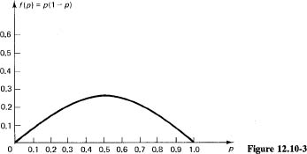
Thus the maximum variance occurs when p = 1/2. A plot of the function
f(p) = p(1 – p)
is given in Figure 12.10-3 and confirms the result. You could use the test
V″ = –2n
to prove that this is a maximum. Thinking about symmetry and the meaning of the symbols shows why this must be true.
Figure 12.10-3
Generalization 12.10-3
A general property of the variance. The mean of a distribution of p(k) is defined by
![]()
and the variance is defined by
![]()
We are, of course, supposing that the sums exist. Expand the square term and spread out the sum into three sums (as we did in Example 12.10-1):
![]()
The middle sum is by definition μ, so the term is –μ2. The last sum by definition is 1, and when multiplied by μ2 it combines with the middle term to give
![]()
When you compare the simplicity of this derivation in the general case with the top of Example 12.10-1 for the specific Bernoulli distribution, you see the advantage of using the general case of a distribution p(k), rather than the details of the particular case at hand. Abstraction often makes things easier and more compact and in the long run perhaps much clearer, because the details are removed and you are looking at the essentials of the situation.
Equation (12.10-7) is of great use in the theory, although you should be wary of using it in numerical work with real data; the roundoff may cause you trouble. The formula says, “The sum of the squares minus the square of the sum of the first powers, each weighted by the probability distribution, gives the variance.”
The mth moment of a distribution is defined by
![]()
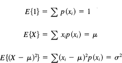
Thus the expected value is the first moment, and the variance is the second moment (about the origin) minus the square of the first moment. The third moment about the mean is called skewness, and the fourth is called kurtosis (see Figure 12.10-4). Higher moments than this are not usually named. Generally, the higher moments are taken about the mean (as is the variance)
![]()
and are called the mth central moments of the distribution p (k).

Figure 12.10-4 Examples of distributions
1. Compute the third moment of the Bernoulli distribution
2. Given the geometric distribution q, pq, p2q, p3q, … , find the first three moments
3. In Exercise 2, find the mean and variance.
12.11 RANDOM VARIABLES
We begin with a sample space of events (outcomes of a trial). We can do no numerical computation with the names of the outcomes of the trials; we need numerical values to assign to the events. It is natural to assign the numerical value of the face of the die to the corresponding outcome. In principle, we could assign any numerical values to any of the faces, but then there might be difficulties in later interpretations.
For a coin, you are apt to assign 0 to one face and 1 to the other face. The expected value would then be
![]()
But you could assign – 1 to one face and 1 to the other. The expected value would then be
Thus the assignment of numerical values to the outcomes of a trial is not unique. The values you assign should be made with an eye toward the later interpretations you are going to make, but for the beginner this is hardly a useful remark!
Again, it is natural to assign the number k to the length of a run of k tosses of a coin until a success. Generally, it soon becomes evident how to assign numbers to the events; indeed, it is so natural that often the student is unaware that this is being done. But it is a logical step that must be taken with an eye toward the final results. With only names for the outcomes, we can do little further mathematics; with numbers properly assigned, we can find many interesting results.
We have been using the notation
E{K}
which looks as if it were a function of K, but on the right-hand side of the equation the dummy variable k of summation occurs. Therefore, the result does not depend on k or K. We need to introduce the corresponding idea behind the notation.
The outcome of a trial cannot be known definitely. It can be any of the possible outcomes; but we need a notation to refer to the trial. For this purpose, we introduce the concept of a random variable (it is not a variable in the usual sense). We use capital letters for random variables (we used K before) to correspond to the lowercase index of the outcomes k. Thus we wrote
![]()
as the expected value of the distribution p(k), and, in general,
as the expected value of the combination f(K) of the random variable K. For example,
![]()
For the general values of the random variable xt (not necessarily integers), we write (supposing, as usual, that the sums exist and are absolutely convergent, Section 20.5)
![]()
As before, we have the moments
We have introduced the notation of X as the random variable whose possible values are the xi. We cannot say which outcome will occur, and we need a notation to talk about the trial. Thus X is the name of the trial, and the various xi's are the possible values of the outcome. The p(xi) are the probabilities of the outcomes. Each time we form a sum, we weight the numerical value assigned to the outcome by its probability of occurrence. It is a matter of rereading much of this chapter to put the results in terms of random variables. Thus you can write, if you wish,
Pk = p(k) = p{X = k}
The idea is simple, once understood, and we have delayed its introduction until it would be comparatively easy to grasp. Sometimes you see the word “stochastic” where we have used “random,” but as far as the author can determine there is no difference among the two schools of notation in what they do with random (stochastic) variables. The values of outcomes you are interested in are multiplied by their probabilities and are then summed over all those of interest.
12.12 SUMMARY
The purpose of this chapter is to introduce the concepts of probability so that they can be used in later sections of the book. They also illustrate the use of the calculus, as well as some of the methods of mathematics. It is not expected that on this first encounter with probability you have mastered all the finer parts of it. You will get constant reviews of the material in the rest of the book. The next chapter will review the ideas in terms of continuous probability.
The main ideas are a trial, especially a Bernoulli trial where the trials are the same and independent of each other; the concept of the sample space of possible outcomes; the assignment of the probability to the events in the sample space; the selection of some subpart of the space; and the computation of various averages over the sample space. Sometimes the probabilities are conditioned on earlier events, and the notion of conditional probability is necessary.
The idea of a random variable was introduced so that we can speak of a trial X whose outcomes are the xi but which xi occurs is unknown. Typically, we have dealt with averages of a random variable over all the possible outcomes, but sums over subsets can be used when appropriate.