20.1 REVIEW
A central concept in the calculus is the idea of a limit. To introduce this idea, we looked (in Section 3.6) at the representation of decimal numbers, including rational numbers. You have the feeling that as you take more and more digits of a number you are getting closer and closer to the limit of the (discrete) sequence of approximations, and you also feel there is a number that is the limit. In Section 3.5 we showed a simple method of approximating the zero of an equation by gradually building up more and more digits of the decimal representation of the number. The existence of a number that is the limit of a convergent sequence was explicitly stated in Assumption 4 of Section 4.5, where we said (but did not define clearly) that we were dealing with convergent sequences.
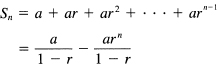
Later, in Section 7.2, we examined more closely the idea of a limit. In particular, given an infinite sum of terms, we examined the sequence of partial sums, and said that the limit of the convergent sequence of the partial sums is the sum of the series. We applied this to the geometric progression
S = a + ar + ar2 + ar3 + …
When |r| < 1, we found that as n → ∞ the sequence of partial sums
approaches the limit
Logically, the limit of a sequence of terms, such as the partial sums of a series, is simpler than the limit of a continuous variable we used in the definitions of the derivative and the integral. Nevertheless, we hastened on to the limit of a continuous variable, and must now return to a closer look at the idea of the limit of discrete sequences. We chose the psychological path, rather than the logical path.
The idea of a limit of a sequence is based on the idea of a null sequence, a sequence that approaches zero. The example of a null sequence we used in Section 7.2 was {1/n} as n approached infinity. This sequence approached zero, although for no finite n does it take on the value zero.
From the null sequence, we reached the general case by noting that the difference between a sequence and its limit must be the null sequence. For example, in the case of a geometric progression, the sequence of partial sums is
![]()
When | r | < 1, the sequence
rn → 0
is a null sequence as n → ∞. It is still a null sequence when multiplied by the fixed number a/(1 – r). Therefore, as n → ∞ the sequence Sn will approach the limit a/(1 – r). Since the limit of a series is defined to be the limit of its partial sums, we say that the geometric series converges to this limit
![]()
This result was applied to a number of cases. In particular, we found that (as we expected) the decimal sequence 0.3333 … 3 (a finite number of 3’s) approached ![]() as we took more and more digits. Slightly more surprising, we found that the corresponding sequence of 9’s approached 1.0.
as we took more and more digits. Slightly more surprising, we found that the corresponding sequence of 9’s approached 1.0.
The idea of a limit requires the sequence to not only approach its limit, but to stay close once far enough along; the difference between the sequence and its limit is a null sequence. We had to make the explicit assumption in Section 4.5 that for any convergent sequence there is always a number that is its limit, because we are not able to prove, in an elementary fashion, that we would not be in the position of Pythagoras when he found that among the everywhere dense rationals there is no square root of 2 (there was no rational number awaiting him). Thus we assumed that, if a sequence is convergent, then there is a number that is its limit.
We further discussed the rules for combining limits and saw them effectively repeated in Section 7.3 for continuous variables (and in L’Hopital’s rule, Section 15.5). In Section 15.4, we looked at Stirling’s approximation to n\ and found that the approximation did not differ from the true value by a null sequence. Thus convergence is a condition that is useful and makes things easy to understand, but we can occasionally handle sequences that are not convergent.
20.2 MONOTONE SEQUENCES
We first examine sequences that are either monotone (constantly) increasing or are monotone decreasing. They are an important class of sequences and shed light on the general situation.
Suppose we have a monotone increasing sequence Sn that is bounded above by some number A. In mathematical symbols,
Sn – 1 ≤ Sn ≤ A
We see intuitively (Figure 20.2-1), that the sequence cannot grow indefinitely (since it is bounded) and cannot “wiggle” (because it is monotone), so surely it must converge. We prove this theorem by contradiction; we assume that it does not converge. To be a bit more careful, the failure to converge implies that there exists at least one number ![]() > 0 such that no matter how far out you go, and no matter which number S you choose as the limit, you can find a difference between the sequence Sn and its limit S that is bigger than the original number
> 0 such that no matter how far out you go, and no matter which number S you choose as the limit, you can find a difference between the sequence Sn and its limit S that is bigger than the original number ![]() . Going beyond this point in the sequence, you can find another such increase, and beyond this new place in the sequence another such increase, and so on, thus as many such increases as you please.
. Going beyond this point in the sequence, you can find another such increase, and beyond this new place in the sequence another such increase, and so on, thus as many such increases as you please.
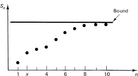
Figure 20.2-1 Monotone increasing sequence
But by picking enough of these, their sum (for a monotone increasing sequence) would add up to more than the distance ot the upper bound, a contradiction that the sequence was bounded. Thus you have the result:
Theorem 20.2-1. A monotone increasing sequence that is bounded above must converge to a limit.
Obviously, the limit is not greater than the bound A and may be below it. A similar result for monotone decreasing sequences that are bounded below is easily found.
For monotone increasing convert sequence Sn of terms, the nth term must approach the limit. The sequence Sn comes from a series of positive (more carefully, nonnegative) terms, when we define
![]()
since the sequence Sn is monotone increasing Sn – Sn– 1 = un ≥ 0. It follows that the nth term un of the series must approach zero. This is a necessary but not sufficient condition for convergence of a monotone series; un → 0 must occur for convergence, but un may approach zero for a nonconvergent series.
Example 20.2-1
The series

cannot converge since the limit, as n approaches infinity, of the value of the general term is 1.
Example 20.2-2
For a > 1, the sequence of partial sums
![]()
converges. We have only to find an upper bound to this monotone increasing sequence of terms Sn. It is easy to see that
![]()
since
![]()
We have, therefore,
![]()
but this last is an infinite geometric progression with the first value 1 and the rate | 1 /a | < 1 ; hence this sum is
![]()
and provides an upper bound on the original series. We have shown that the given series converges, although we do not have a value for the sum, only an upper bound.
This is a special case of a fairly obvious result.
Theorem 20.2-2. If each term of a series of nonnegative terms is bounded by the corresponding term of a second series, and if the second series converges, then the first series must converge.
Proof. In mathematical symbols, if (1) {an} is a sequence of nonnegative numbers, (2) an ≤ bn, and (3) Σbn converges, then Σan converges. The proof goes along the lines given in the above example. The Σbn provides an upper bound to the monotone increasing sequence
![]()
If the sum of a series of nonnegative terms does not converge, then necessarily it approaches infinity. Such a series is said to diverge.
Some of the results we have just obtained refer to more general series than monotone series. For example, the result that if a series converges then necessarily un → 0 is such a result.
Theorem 20.2-3. If a series of partial sums Sn converges, then un → 0.
Proof. To prove this we first note that
Sn − Sn − 1 = un
Now we write (where S is the limit of the sequence Sn)
![]()
But since the series is assumed to be convergent, both of these terms approach zero; therefore, un must approach zero.
Before going on, we need to note one more obvious theorem.
Theorem 20.2-4. The convergence of any series is independent of any finite starting piece of the series, although of course the sum depends on it.
Proof. No matter how many terms you take of the beginning of the series, be it 100, 1000, 1 million, or any other finite number, the sum of them is also finite. If the series converges, then the tail of the series must also converge; and if the series diverges, then, since the sum of all the terms is infinite, the tail must total up to infinity independent of the sum of the first part you took separately.
This result is useful since it says that when determing the convergence or divergence of a series of terms, positive or otherwise, you need only study the values past any convenient point, and you can ignore any early part of the series you wish. If the series settles down to positive terms past some point, then it can be treated as a series of positive terms.
1. Does Σ 2/(3 + 1 /n) converge?
2. Show that Σ a/(1 + bn) converges for b > 1.
3. Show that Σ a/(bn + (− l)n) converges for b > 1.
4. If un → 0 and = Sn Σ (un+1 − un), then Sn converges.
20.3 THE INTEGRAL TEST
The beginning student in infinite series soon begins to wonder why so much attention is paid to whether or not the series converges and so little attention to the number it converges to. The answer is simple; it is comparatively rare that the sum of a series can be expressed in a convenient closed form. It is much more likely that an integral can be done in closed form than can an infinite series be summed in closed form. The reason for this is that for integration we have a pair of powerful tools, integration by parts and change of variable; for infinite series we have only summation by parts (Section 20.4), and there is no comparable change of variable with its Jacobian. Thus, again, we see that, in a certain very real sense, discrete mathematics is harder than is the continuous calculus; we can less often expect to get a nice answer to the equivalent problem.
This being the case, it is natural to try to use integration as a tool for testing the convergence of series. (In Section 15.4 we used integration as a method of approximating finite and infinite sums.) We have the following result.
Theorem 20.3-1. Given the monotone series of positive terms un
![]()
then the integral
![]()
converges or diverges with the sum, provided that for all x the function u(x) is monotone decreasing [with un = u(n) of course].
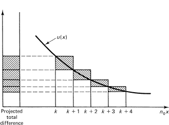
Proof. We have only to think of the fundamental result that the integral is the limit of the sum and draw the figure for the finite spacing of Δx = 1 (Figure 20.3-1). We see the upper and lower sums (over the monotone part, which is all that matters) bound the integral above and below. Their difference is not more than the projected total on the column to the left, not more than the size of the first term we are considering. We write
Figure 20.3-1 Integral test
upper sum = lower sum + difference
We also have
upper sum ≥ integral ≥ lower sum
If the integral diverges, then the upper sum diverges and this differs from the lower sum by a fixed amount, so the lower sum must also diverge. Similarly, if the integral converges, then the lower sum must converge and so must the upper sum. In this simple case of only determing the convergence or divergence of the series, and not its actual sum, it is not necessary to use the more refined methods of estimating integrals by sums that we used in estimating Stirling’s approximation to n! (Section 15.4).
When examining this theorem, we see the condition that u(x) must be monotone decreasing. Is it not enough that the original terms un be monotone decreasing? True, the proof we gave required u(x) to be monotone, but perhaps another proof might not. A few moments’ thought produces the example [u(x) is monotone]
u1(x) + sin2 πx
which shows that although u1(x) takes on the values of the terms of the series un at the integers, nevertheless the total area under the curve is infinite since each loop of the sin2 πx has the same finite area. Thus the monotone condition is necessary (at least some such constraint is necessary).
Example 20.3-1
The p–test. The series
![]()
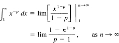
occurs frequently. The corresponding integral (and we do not care about the lower limit since the convergence or divergence depends solely on the tail of the series), p ≠ 1, is
If p > 1, then the limit is 1 /(p − 1) since nl − p → 0. Next, if p < 1, the limit is infinite. Hence the series converges if p > 1 and diverges if p < 1. For the case p = 1, we can use the integral test and deduce the divergence from
![]()
As an alternative approach we can look back to the approximation of Example 15.4-3:
![]()
Since In n → ∞ as n → ∞, it follows that the harmonic series
![]()
diverges to infinity.
Give the convergence or divergence of the following series.
1. Σ 1/ ![]()
2. Σ 1/n
3. Σ 1/n3/2
4. Σ 1/n2
5. For ![]() > 0, Σ 1/n1 +
> 0, Σ 1/n1 + ![]() Σ 1/nl –
Σ 1/nl – ![]()
20.4* SUMMATION BY PARTS
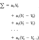
Summation has a discrete analog corresponding to integration by parts. Suppose we have
![]()
We write
![]()
The series may now be written in the equivalent forms (since ![]() Vk − 1 = Vk − Vk − 1 and
Vk − 1 = Vk − Vk − 1 and ![]() V−1 = v0)
V−1 = v0)
![]()
In this last form it resembles the usual integration by parts. If we write this out in detail, we have (remember that V0 = v0)
Rearranging this in terms of the V's, we get
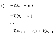
Hence we have, using ![]() uk = uk+1 – uk, and writing v–1 = 0,
uk = uk+1 – uk, and writing v–1 = 0,
![]()
which resembles integration by parts.
Just as we use integration by parts to eliminate powers of x, so too can we remove powers of n from a summation. The elimination of In and arctan terms by integration by parts in integration does not work for series. The application of parts twice and finding the same summation again will work as it did in exponentials times sines and cosines.
Example 20.4-1
Consider the simple example
![]()
Using (20.4-1), we set uk = k and ![]() Vk – 1 = ak. Then
Vk – 1 = ak. Then
![]()
![]()
and the sum is now easily done by breaking it up into two terms, the second of which is a simple geometric progression (again). We leave the details to the student.
EXERCISES 20.4
1.* Show that Σ(1/2k) sin ka = {2 sin a – 2–n[2 sin a(n + 1) – sin a]}/{1 + 8 sin2 (a)/2}
2. Sum Σ k cos kx
20.5 CONDITIONALLY CONVERGENT SERIES
Many series of interest are not of constant sign, but have terms that may be positive or negative. Among these is the frequently occurring special class of alternating series whose terms alternate in sign.
Example 20.5-1
The alternating harmonic series is defined by
![]()
To sum this series, we recall, again, the result of Example 15.4-3:
![]()
as n approaches infinity. Now consider
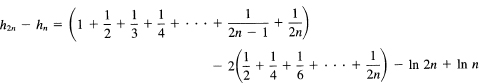
where for the second part (from hn) we have put a factor of 2 in front and compensated by dividing each term by 2. The result of adding these two lines changes the sign of all the terms with an even denominator; and this is the alternating harmonic series pattern for S2n. But since both h2n and hn approach the same limit γ, their difference must approach zero. Hence
![]()
The S2n+1 approach the same limit as the S2n since the difference 1/(2n + 1) → 0. Hence the alternating harmonic series converges, while the sum with all positive terms diverges. We say that such a series is conditionally convergent.
A useful theorem for dealing with alternating series whose terms are monotone decreasing in size is the following:
Theorem 20.5-1. If the un are monotone decreasing to zero, then the series
![]()
converges.
Proof. The proof is easy. (Note this time we begin with u0 as the first term; hence there are small differences from the proof for the alternating harmonic series.) We write the even-indexed partial sums of the series out in detail:
![]()
From this we have that u0 is an upperbound of S2n (since each parentheses is a nonnegative number). Now writing the series in the form
![]()
we see that these partial sums form a monotone increasing sequence that is bounded above by u0, and hence must converge. Since
![]()
and the u2n+1 → 0, it follows that the partial sums for odd and even subscripts converge to the same limit. Therefore, the series converges.
If the series
![]()
converges, we say that the series is absolutely convergent.
We need to prove the result:
Theorem 20.5-2. If a series (alternating or not) is absolutely convergent, then it is also conditionally convergent.
Proof. It is not completely obvious that the positive and negative terms could not make the sum of the series oscillate indefinitely while still remaining finite in size, and thus the series would not converge. To show that this is impossible, we use a standard trick and define two series, one Pn consisting of the positive terms and one Qn of the negative terms. To be able to name the terms easily, we supply zeros for the missing terms in each of the defined series. Thus we define
![]()
We have from the definition of Pn and Qn for all finite sums
![]()
From the absolute convergence of the series, we see that
![]()
Hence each sum on the left (being positive) must converge separately, since each is separately bounded above (by the sum on the right) and is monotone increasing. Now Σ un is the difference of two convergent series and hence also must converge.
Some of the results we proved for series with positive terms apply equally well for series with general terms. Thus for convergence it is necessary that un → 0, as well as the fact that the convergence or divergence of a series depends only on the behavior of the tail of the series, and not on any finite number of beginning terms.
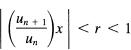
The main series for which we know the sum is a geometric progression when | r | < 1. Given any other series, we now ask how we can get the terms of the given series dominated by those of some suitable geometric series. The following ratio test is based on the convergence of a geometric series. Suppose we have a series un such that
![]()
as n approaches infinity. Then there is another number r1 < 1 such that r < r1 < 1. Next, from the limit we deduce that sufficiently far out
![]()
for all n larger than some starting value n0. This means that for any n ≥ n0
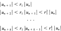
Thus the original terms um (m > n) are dominated by the corresponding terms of a geometric progression with rate r1 < 1. This geometric progression is a convergent series (all, of course, sufficiently far out in the series). Hence we have the following ratio test.
Theorem 20.5-3. If, for a series of positive terms,
![]()
for all sufficiently large n, then the series converges; and if
![]()
for all sufficiently large n, then the series diverges. This can be stated in the limiting from; if as n approaches infinity
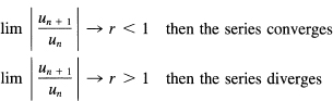
and if the limit is 1, no conclusion can be drawn.
The limiting form is slightly more restrictive than is the inequality form, but the difference is not great; un + 1/un need not approach a limit and the result is true. The proof for the divergent part is very similar to that of the convergent part.
If the limit of the ratio is 1, then nothing definite can be concluded since we have both convergent and divergent series with the limit equal to 1 (as we will soon show, Example 20.6-1).
There is an important theorem concerning conditionally convergent series; if you permit a rearrangement of the order of the terms in the series, you can get any answer you wish! To prove this, we go back to the notation of Pn being either the corresponding positive term or else 0, while the Qn refer to the negative terms. For a conditionally convergent series, both the series in Pn and Qn must diverge to infinity.
Now we pick a number, say a positive number, that you want to be the limit of the rearranged series. First, we add terms from the Pn until we pass the given number. Next, we subtract terms from the Qn until we pass under the number. Then we add terms from the Pn until we are again over; then subtract terms from the Qn, and so on. Since the series was originally conditionally convergent, the terms of both the Pn and the Qn must approach zero. Thus the alternate going above and below the chosen number will get smaller and smaller. On the other hand, since each diverged to infinity, we cannot run out of numbers to continue the process. The series, in the order we are taking the terms, will converge to the given number.
Notice that in the process we will displace numbers arbitrarily far from their original position in the series. If you restrict yourself to a maximum displacement of terms, then this result is not true; it depends on gradually displacing terms farther and farther from their original position.
This theorem explains why in defining the expectation of a random variable we included the absolute value of the random variable; we may not have a natural order, and if the series, or integral, were conditionally convergent, then depending on the order we chose we would get different results when we allow nonabsolute convergent series or integrals.
1. Does ![]() converge?
converge?
2. Give the interval of convergence of ![]()
3. Is ![]() absolutely convergent?
absolutely convergent?
4. Is ![]() absolutely convergent?
absolutely convergent?
5. Write an essay on absolute convergent and conditional convergent integrals.
20.6 POWER SERIES
A particularly important class of infinite series is
![]()
or, what is almost the same thing,
![]()
The difference is merely a shift in the origin of the coordinate system. They are both called power series. In this section we treat only the first form, but see the exercises for the second form.
The convergence can be examined using the ratio test. For the first series, we have the condition that
for convergence, and similarly for divergence. The series with x – x0 behaves simi larly.
Example 20.6-1
For the geometric progression (note the change in notation from r to x)
the ratio test gives
![]()
as we earlier found.
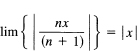
For the series
![]()
the ratio test gives
![]()
Hence the series converges if |x| < 1 and diverges if |x| > 1. At |x| = 1, the series cannot converge since the nth term does not approach zero. The interval of convergence is – 1 < x < 1.
For the series
![]()
we get
which converges for |x| < 1 and diverges for |x| > 1. At x = +1, the series is the harmonic series
![]()
which diverges (Example 20.3-1), and at x = –1, you have the alternating harmonic series
![]()
which converges (Example 20.5-1). The interval of convergence is –1 ≤ x < 1. Thus we have shown that at the ends of the interval of convergence the series can sometimes converge and sometimes diverge. It is easy to see (Example 20.3-1 with p = 2) that the series
![]()
converges at both ends of the interval – 1 ≤ x ≤ 1.
We need to prove the following important result.
Theorem 20.6-1. If a power series converges for some value x0, then it converges for all x such that
![]()
Proof. The proof follows immediately from the observation that if the series converges for x = x0 then the nth term must approach zero. Hence past some point we must have
![]()
We can therefore write, for |x| < |x0|,
![]()
and the series converges. Thus we always have, for power series, an interval of convergence, which can be (1) closed at both ends, (2) open at one end, or (3) open at both ends. The ends of the interval must be separately examined since, as we showed in Example 20.6-1, any particular situation can arise.
Can we integrate a power series term by term? If we stay inside (avoid the ends) the interval of convergence, then from the convergence assumption of the power series we can find some place far enough out so that the remaining terms total up to as small an amount as you wish. And in this closed interval there is a farthest out point that will apply for all the x values in the interval (see Section 4.5, assumption 3). When we integrate term by term the approximation of the finite series, the error will be multiplied by a fixed finite amount, the length of the path of integration. Thus the difference between the integral of the function and the integral of the finite series can again be as small as required. We conclude that we can indeed integrate a power series term by term and expect that the series will represent the corresponding integral, provided the length of the path of integration is finite and lies inside the interval of convergence.
Can we differentiate term by term? It is not so easy to answer because we see immediately that the differentiation process produces coefficients that are larger than the original series. But if the differentiated series converges, then, reversing the process and integrating it, we can apply the above result. Thus, if we differentiate a power series term by term and the resulting series converges, it is the derivative of the function.
Find the interval of convergence.
1. Σ xn/(n2 + 1)
2. Σ (x – x0)n
4. Σ (x – x0)n/n2
20.7 MACLAURIN AND TAYLOR SERIES
When dealing with power series, it is often convenient to change notation. Suppose we denote the power series by
![]()
(We set un = an/n!). We see immediately that for x = 0 we have
![]()
If we formally differentiate the series and then set x = 0, we get
![]()
A second formal differentiation gives
![]()
and in general we will get
![]()
Therefore, the series can be written in the form
![]()
This is the Maclaurin (1698–1746) series.
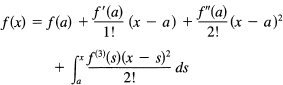
If, instead of evaluating the derivatives at the origin, we used the point x = a, we would have the corresponding Taylor (1685–1731) series
![]()
There has been the tacit assumption all along that both the differentiated series converged, and that the final series would represent the original function. Is there anything we can do to find the error term corresponding to a finite number of terms? It happens that there is. The method depends on integration by parts, and we have seen part of the formula before (Section 11.7 on the mean value theorem). We start with the obvious expression
![]()
where we have used the dummy variable of integrations to avoid confusion with the upper limit x. We pick the parts for the integration
dU =f'(s) ds, V = – (x – s)
Notice the peculiar form we picked for the V. Certainly the derivative is correct, and by picking this form, then when s = x the upper limit of the integration will drop out. We have
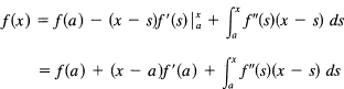
We integrate by parts again, this time picking
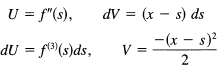
and have, after putting in the limits of integration,
Either by induction or the ellipsis method, after n stages we will have
![]()
where the remainder Rn is
![]()
If Rn → 0 as n → ∞, then the difference between the function and the sum of the first n terms of the power series will approach zero. Thus the power series will both converge and represent the function; the difference approaches zero.
The integral (20.7–4) can be reworked using the mean value theorem for integrals (Section 13.3). The factor (x – s)n–l is of constant sign in the interval [a, x] of integration (even if x < a). As a result, we have
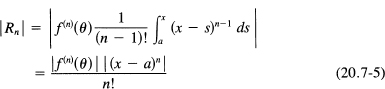
This is the derivative form of the remainder.
![]()
for some constants Mn. Then we have
![]()
If this approaches zero as n → ∞, then the expansion approaches the value of the function for the corresponding values of x. Unless Mn grows at least as fast as n!, then the factorial in the denominator will cause the whole term (for fixed x) to approach zero as n → ∞. Therefore, the series expansion will converge and represent the function.
Thus we have the following important class of cases: if the derivatives are bounded by the corresponding terms of a geometric progression (which need not converge), then the series converges.
20.8 SOME COMMON POWER SERIES
The ability to find the general term of the Maclaurin and Taylor series evidently depends directly on the ability to find the nth derivative of a function. This we can do only in selected cases, which are fortunately the cases of main importance. For other functions we can get only as many terms as we are willing to compute derivatives, one after the other.
Example 20.8-1
For the function y(x) = eax, we have

and, in general, the nth derivative acquires a coefficient an. If we expand this function y(x) = exp ax about the origin, we have for the derivative values
1, a, a2, ….. an, ….
and hence the expansion
![]()
The ratio test gives convergence for all x, since
![]()
approaches 0 for all finite values a and x.
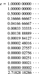
The special case of x = 1/a gives
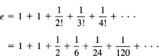
from which it is easy to compute a value for the constant e.
We also need to check that Rn approaches zero as n → ∞. The factorial in the denominator guarantees this.
Example 20.8-2
The other special case, x = –1/a, leads to series
![]()
whose corresponding sum is
e-1 = 0.367894412…
This number arose in an earlier matching problem and was the limit of no match occurring when pairing off two sets of n corresponding items.
Example 20.8-3
Find the Maclaurin expansion of y = sin x. We have

etc.
The corresponding values of the derivatives at x = 0 are
0, 1, 0, –1, …
and these values repeat endlessly. Thus the expansion is
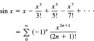
Again the ratio test shows that the series converges for all values, and the further test shows that Rn → 0.
It should be noted that if we can find a convergent power series representation of a function then we have the values of the derivatives at the point of expansion.
Example 20.8-4
For |x| < 1, the fuction
![]()
Hence at x = 0 the nth derivative of y = 1/(1 – x) is n!
1. Find the Maclaurinexpansion of ln (1 + x).
2. Find the Maclaurinexpansion of ln (1– x).
3. Find the Maclaurinexpansion for y = ln [(1 + x)/(1 –x)].
4. Find the Maclaurin expansion of cos x.
5. Find the first three terms of the expansion about x = 0 of y = tan x.
6. Use the Maclaurin expansion of ln (1 + x)/(l – x) from Exercise 3. For x = 1/3, this gives ln 2. Evaluate it for the first three terms. What value of x gives ln 3?
7. Using partial fractions and Example 20.8-4, find the values of the derivatives at the origin of the function y = 1/(1 – x2).
20.9 SUMMARY
The topic of infinite series is vast, and we have only touched on the matter. The convergence of an infinite series is made to depend on the convergence of the corresponding sequence of partial sums Sn. We studied, in turn, null sequences, monotone sequences, and then the general case. This is typical of doing new mathematics; the simpler cases are attacked first, and from them the general case is approached.
The power series is especially important, and we examined the expansion of a few of the common elementary transcendental functions, exp (x), sin x, cos x, and ln (1 + x); the last two are in the exercises. In the next chapter we will further examine this important topic of representing functions as infinite series.