11.1 HISTORY
The integral calculus was actually developed before the differential calculus. It arose from the problem of finding areas and volumes defined by mathematical expressions. In the early stages each particular area or volume problem was solved by a suitable trick. The great progress occurred when systematic methods were introduced and the fundamental theorem of the calculus was discovered. This theorem says that differentiation and integration are inverse processes one to the other (much as multiplication and division are inverse processes).
Experience seems to show that when presenting the calculus for the first time it is preferable to put the differential calculus before the integral calculus (which is what we have done). Nevertheless, mathematically it is the other way around; the rigorous approach is easiest from the integration side. We will base our approach to the integral calculus on the idea of area, and then extend, generalize if you prefer, the idea to a broader context. It is necessary, therefore, to first review your beliefs about area.
11.2 AREA
You emerge from elementary Euclidean geometry with the belief that the area of a square is proportional to the square of the side. For example, you can see directly that a square 10 by 10 is composed of 100 congruent unit squares (Figure 11.2-1). It is conventional to take the constant of proportionality as being 1. Hence, the measure of the area of a square is the square of the side.
Next, you believe that the area of a finite sum of nonoverlapping areas is the sum of the individual areas, in short that area is additive for finite sums of areas. Along the way you also agree that area is to be measured by a positive number, with 0 being the area of “nothing.”
You also believe that congruent figures must have the same area; you would be logically embarrassed if you did not, since congruent figures are interchangeable as far as area is concerned.
Finally, and this is an assumption, too, you probably believe that every figure has a unique area. This means, for example, that you are assured, when you compute it, that the area of a triangle is independent of which side you pick for the base.
Figure 11.2-1 A 10 by 10 square
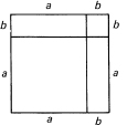
Figure 11.2-2 Square (a + b)2
Looking at Figure 11.2-2, you can see that the algebraic identity
A = (a + b)2 = a2 + 2ab + b2
corresponds to a geometric identity. This identity says that the whole square is the sum of the two squares (of area a2 and b2), plus the two, congruent rectangles. The two congruent rectangles have necessarily the same area. From this you deduce that the area of a single rectangle of sides a and b must be
A = ab
The diagonal of a rectangle (Figure 11.2-3) divides it into two congruent triangles, and therefore each of these right triangles must have the area
![]()
Now any triangle, right or otherwise, can have a perpendicular dropped from a vertex to the base, which cuts the given triangle into two right triangles (Figure 11.2-4). You can either make sure that the vertex chosen is the largest angle, or else discuss the fact that, if the perpendicular (the altitude) falls outside the triangle then you are talking about the difference between the areas of the two triangles. Either way, from the assumptions you come fairly directly to the formula for the area of a general triangle:
![]()
Figure 11.2-3 Rectangle as two triangles
![]()
Figure 11.2-4 Triangle
![]()
Next, any plane closed figure that does not cross itself and is bounded by a finite number of straight lines may be decomposed into triangles (Figure 11.2-5). At any convex angle (less than 180° as seen from the inside of the region, and there is always at least one such angle), you can, as in Figure 11.2-6, reduce the number of sides by 1 when you draw the third side of the triangle since what is left to triangulate has one less side. The triangulation is not unique (but you can see that it can always be done). Since you assumed that the area is unique, it does not matter just how the triangle decomposition is done; the resulting area will be the same for a given figure (again, having a finite number of sides).
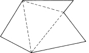
Figure 11.2-5
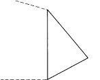
Figure 11.2-6
It is when you face the area of a circle, for example, that you need to think. It soon becomes evident that some new definition, an extension of the old definition, of area must be made for regions bounded by other than straight lines. No matter how you choose to extend the definition, it should be consistent with the earlier definition. In short, it is necessary to make an extension of area to new shapes, a standard situation in creating new mathematics.
EXERCISE 11.2
1. Draw a right triangle and drop a perpendicular from the right angle to the hypotenuse. This divides the original triangle T1 into two triangles T2 and T3. The three triangles are similar. Derive Pythagoras’ theorem.
11.3 THE AREA OF A CIRCLE
The simplest figure that has curved sides is the circle. While Euclid’s Elements proves that the areas of circles are to each other as the squares of their respective sides, nowhere does he discuss the number π; nowhere does he get the measure of the area.
The historical approach to finding the area of a circle is to inscribe (inscribe means draw inside) a regular polygon in the circle and then compute the area of the polygon. This area is taken to be a lower bound on the area of the circle. Archimedes by a clever device doubled the number of sides of the inscribed polygon (see Figure 11.3-1). Then he again doubled the number of sides, and so on. He then took the limit of the area of the sequence of inscribed polygons to be the area of the circle.
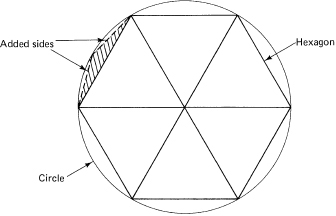
Figure 11.3-1
There were endless arguments as to whether the polygon became the circle in the limit or not. There was confusion between (1) the area of the inscribed polygons approaching the area of the circle, and (2) various properties of the perimeter (straight line segments) approaching a constantly curving circle. We have learned to avoid such questions and confine ourselves to the question, “Does the area of the inscribed polygons get arbitrarily close to the area of the circle?”
But we are not as sure as we might be when we merely use this approach of inscribing regular polygons; instead, we propose to also circumscribe (circum-, around) a regular polygon around the outside of the circle (Figure 11.3-2) and again let the number of sides be doubled indefinitely. If the two areas, that of the inscribed and that of the circumscribed polygons, approach the same number, then it seems reasonable to take this common number as the area of the circle. Note that we are actually defining what we mean by the area of a figure with curved sides.
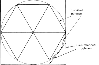
Figure 11.3-2
This approach is a tedious piece of special algebra and trigonometry to carry out for a circle. What is important is both the plan for finding a common limit and the realization that a new definition is required to deal with areas bounded by curved lines. Instead of finding the area of a circle, we will start finding the areas under the parabolas (a generalization of y = x2),
y = cxk (k >0)
and later (Examples 11.9-4 and 16.7-1) find the area of a circle in a simple fashion.
11.4 AREAS OF PARABOLAS
Example 11.4-1
Given the family of parabolas
![]()
the simplest case, k = 1, is a straight line. This forms a triangle whose area we already know (we can use this case as a check on what we are doing). We have
y = cx
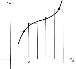
To estimate the area under the curve, above the x-axis, and to the left of the vertical line x = a, we first inscribe (see Figure 11.4-1) a sequence of narrow rectangles, and then examine the limit as the number of rectangles approaches infinity (gets arbitrarily large). Take the width of each rectangle to be
![]()
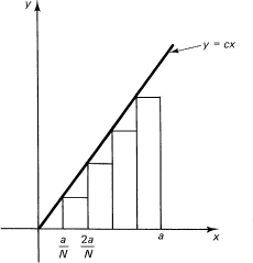
Figure 11.4-1
where N = the number of rectangles. From the figure we have the inscribed area AI(N) [AI(N) depends on N, of course].
![]()
But this can be simplified by factoring ac/N from each term:
![]()
We know the sum of the consecutive integers from Section 2.3 (N – 1 = n in the formula), and we also can eliminate the Δx = a/N. We get the area of the inscribed polygons:
![]()
Rearranging this, we have
![]()
and this approaches the limit A1:
![]()
as N approaches infinity. We recognize that this is the correct answer for a triangle. But let. us persevere in our approach and compute the area of the circumscribed set of rectangles.
For the circumscribed set of rectangles, we get exactly the same thing (see Figure 11.4-2), except that the sequence of rectangles begins with the height proportional to 1 and goes on to height proportional to N, instead of beginning with the 0 and going to N – 1. We have, therefore [compare with Equation (11.4-2)], the circumscribed area
![]()
and the corresponding sum is [compare with Equation (11.4-3)]
![]()
Rearranging this, we have
![]()
which again approaches (11.4-4):
![]()
Thus the limit of both the inscribed and the circumscribed areas is the same. We have tested the approach on a known result and found that it works correctly.
When you consider the difference between the inscribed and circumscribed sums, (11.4-5) and (11.4-6), you see that it is
![]()
and that as N → ∞ the difference must approach zero.
Example 11.4-2
The next case is k = 2,
y = x2
We have chosen to ignore the front constant c (since from Example 11.4-1 you see that it will simply factor out of everything, and remain in front of the final answer). From Figure 11.4-3 you have the inscribed area under the curve, above the x-axis, and to the left of the line x = a. The area is
![]()
After factoring out the common factors and replacing Δx by its proper value (a/N) in terms of N, you have [compare with (11.4-2)]
![]()
The circumscribed area is correspondingly [compare with (11.4-5)]
![]()
(the difference being again the end terms). For the inscribed area, from Example 2.3-2, we have, on substituting for the sum of the squares of the consecutive integers (n = N – 1),
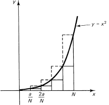
Figure 11.4-2
and for the circumscribed area (n = N),
![]()
It is easy to see that as N → ∞ both expressions approach
![]()
Thus we take a3/3 as the area under the second-degree parabola. From these two examples (plus just plain thinking), we are inclined to accept the definition of the area as being this common limit of the areas of the inscribed and circumscribed polygons.
Generalization 11.4-3
We naturally turn next to the general case of
y = xk (k = positive integer)
(see Figure 11.4-4). Again, we will find the area under the curve, above the x-axis, and to the left of the vertical line x = a. We proceed slowly. For the inscribed area, we will get
![]()
and, factoring out the common quantities while also replacing Δx by a/N, we get for the inscribed area [compare with (11.4-2) and (11.4-7)]
![]()
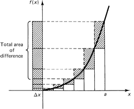
Figure 11.4-3
Using the sum of the kth powers of the consecutive integers from Generalization 2.5-2, we have
![]()
which is a polynomial of degree k + 1 in N – 1 (N = the number of rectangles). We rearrange this:
![]()
As N goes to infinity, all the terms in the bracket except the first approach zero, and we get the limit,
![]()
For the circumscribed sum, we will have one more term in the sum of the kth powers. This approximation produces an N in place of N – 1 in the sum:
![]()
but otherwise it is the same. In the limit the result is the same. Thus the circumscribed polygons and inscribed polygons both lead to the same limit (of the two approximate areas):
![]()
Looked at in another way (Figure 11.4-4), the difference between the areas of the sums for the circumscribed rectangles and the inscribed rectangles is the single term
![]()
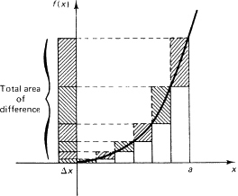
Figure 11.4-4
Therefore, as N approaches infinity, the difference between the circumscribed and inscribed areas must approach 0; both the upper and the lower sums must approach the same limit, and thus they serve to define the area under the curve y – xk out to x = a. These are often called the Riemann (1826–1866) upper and lower sums.
EXERCISES 11.4
1. Carry out the details for the function y = x3.
2. Carry out the details for the function y = x4.
11.5 AREAS IN GENERAL
We now turn to the case of a general function and the area under it (assuming that the function is above the x-axis). Thus we are given a function
y = f(x)
We assume that this is composed of a finite number of pieces each of which is monotone increasing or monotone decreasing (not strictly monotone, but only monotone). See Figure 11.5-1. These are the famous Dirichlet (1805–1859) conditions. Since they permit discontinuities and other reasonable behavior, we are allowing a broad enough class of functions to meet most elementary needs when modeling the real world.
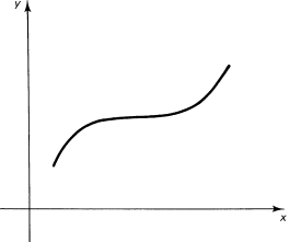
11.5-1 Monotone increasing function
We consider the area under one piece of this function, and argue that if we can find this area then, because the area is additive for any finite number of pieces, we can find the area under the whole function. Suppose we begin at x = a and go to x = b, where a < b. Figure 11.5-2 shows one piece of the function. For convenience, we assume that in this interval f(x) is monotone increasing. The changes for a monotone decreasing function are trivial.
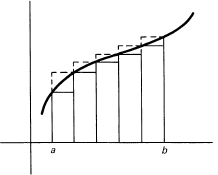
Figure 11.5-2
The difference between the upper sum AU(N) and the lower sum AL(N) for equally spaced rectangles will be (Figure 11.5-3 shows these differences projected into a single column on the left)
![]()
But
![]()
Therefore, the difference between the upper and lower sums is
![]()
which must approach zero in the limit as N → ∞. Thus the method of upper and lower sums defines a common limit to associate with the concept of the area under the continuous monotone curve y = f(x) between the two limits a and b.
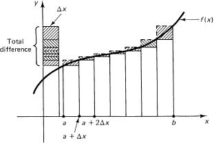
Figure 11.5-3
To generalize the idea of the approximating upper and lower sums of a monotone continuous function, we see first that we need not require that all the rectangles have the same width; they can be of any convenient widths, provided the widest one approaches 0. The projection of all the differences multiplied by their widths onto one column will give a bound:
![]()
(see Figure 11.5-4). Thus we have some flexibility in picking the interval widths. Any set of rectangles will do, provided the widest interval approaches 0 in the limit. The difference between the upper and lower sums will be bounded by
![]()
The upper and lower sums will therefore approach a common limit, which we call the area under the curve. Further thought shows that the upper and lower sums need not use the same intervals.
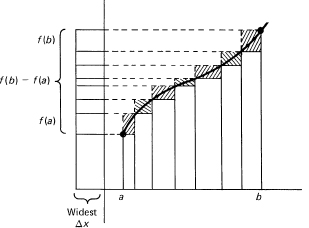
Figure 11.5-4
As a further generalization, we see that we can estimate the sum of the rectangles for a monotone continuous piece of the function by choosing the height of the ith rectangle corresponding to any value θi (Greek lowercase theta) of the function in the ith interval:
![]()
The estimate for the sum (which in the limit is to approach the area) is now
![]()
where the maximum difference xi – xi−1 approaches zero in the limit. Hence (Figure 11.5-5), we have for a monotone increasing continuous function
![]()
Figure 11.5-5
In mathematical symbols (using the notation of Section 9.9),
![]()
For a monotone decreasing function, the inequalities of this last equation are obviously in the opposite direction. Due to the continuity of f(x), the three function values and f(xi-1), f(θi) and f(xi) all approach the same value in the limit, and hence we see again that the middle sum must also approach the common sum of the two ends as N approaches infinity.
The upper and lower sums are called Riemann sums because he was the first to make general the idea of an area mathematically rigorous. The common limit of the upper and lower sums is called the integral (integrate means to make into a whole). Since his time the concept of an integral has been further generalized, but that development lies beyond the needs of this course.
From the areas of the monotone pieces of the function, we obtain, by simple addition, the area under the whole curve (consisting of a finite number of the pieces of monotone continuous functions).
Thus we see that the limit of the sum can be defined using any arbitrary intervals (as long as the largest approaches 0 as N approaches infinity), and we can pick any typical value in the ith interval as the height of the corresponding rectangle. We are not limited to equal spacing and picking particular values in each interval, nor must the intervals chosen for the upper and lower sums be exactly the same.
Further thinking about what we have done shows that actually we are computing the limit of a sum; the word “area” was only a colorful way of referring to the problem. Integration is actually the computation of the limit of a sum that is chosen in a rather flexible manner; it is not the rigid thing we began with. This is very typical in mathematics; an idea that arises in a specific context is gradually generalized until the original idea is merely a very special case.
We assumed that the two limits between which we were computing the area were different. It is a natural extension of the idea of area (and the generalizations we have made from it) to say that if
b = a then the integral (area) = 0
A further extension is that if b < a then the integral (the limit of the sum) is to be negative, since the Δxi will be negative. Similarly, if the function is below the x-axis and the Δxi is positive, we would naturally call the integral negative. Finally, it follows that if b < a and f(x) < 0 then the integral would again be positive, since it would be the limit of a sum of positive terms.
Notice that we began by claiming that area was measured by a positive number or 0, and now we are admitting negative areas. The contradiction is only apparent; we still feel that areas are nonnegative but that at times it is convenient to call an area negative. We made the positive area convention when we first examined areas. Now, due to the generalizations we have made, from our original idea of area to the idea of a limit of a sum, it is convenient to allow negative areas; otherwise, we would be forced to limit ourselves to functions that were nonnegative and sums where b ≥ a. We could easily fix up the contradiction if we wished, but that would later force us into a lot of circumlocutions when we wanted to discuss problems where the areas (sums) cancel. We have only to keep in mind the apparent contradiction and watch for any foolishness that may emerge when we are careless. In a sense, we have extended the idea of area, and this generalization needs to be watched to see all the consequences.
We now introduce the usual notation. The limit of the sum is suggested by the elongated S (Sum) that begins the symbol. The letters a and b at the bottom and top of this elongated S are the limits of the range we are using. The next piece is the name of the function f(x). Finally, we have the name of the variable with respect to which we are summing, the differential dx. We write it in the differential form as
![]()
This is called the integral from a to b of the function f(x) with respect to the variable x. In words, “the integral from a to b of f(x) dx.”
The integral can be thought of as an operator, like d/dx, but in the form
![]()
where the … is the place for the name of the function to be integrated with respect to the variable x.
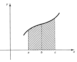
If b lies between a and c, then it is clear that (see Figure 11.5-6)
![]()
Figure 11.5-6
This is merely the statement that adjacent nonoverlapping intervals add properly for sums as well as for areas. Due to our use of the algebraic sign of areas, it is still true when b is not between a and c (provided the integrals exist). With all this formal apparatus, we can now find sums and areas by a uniform method, rather than a collection of artificial special techniques.
We remind you again, we generalized our primitive ideas about areas until we found that a suitable limit of a sum is the integral of the function. Areas are only a special application of the idea of an integral.
11.6 THE FUNDAMENTAL THEOREM OF THE CALCULUS
The great discovery that made the calculus a “calculus” (a routine process) is that it is sensible to ask, “What is the derivative of the integral?” We now think of the area under a function y = y (x) (or any of the extensions of this idea) as depending on the upper limit of the range of the integration (set b = x):
![]()
Before going on, it is convenient to remove a possible source of confusion. The x in the above integrand is a dummy variable in the sense that if we used any other letter for the variable x, say the letter t in
f(x)dx
then in its place we would have
f(t)dt
and we would have the integral
![]()
The area (or, more generally, the limit of the sum) would be the same. The reason is simply that the expression says that the variable of summation goes from the lower limit of integration a to the upper limit x. This change of the dummy variable of integration is exactly the same as we have for summation:
![]()
Whether we use n or m makes no difference in the answer. If we do not make this change in notation for the integral (11.6-1), we will become confused with the different meanings of x. In the old form it was both the variable of summation and the value we used as the upper limit in the final sum. In the new form we are summing and then taking the limit of a set of function values times the corresponding interval widths, depending on the dummy variable t, and using x as the upper value.
We now ask, “What is the derivative of this integral?” What is
![]()
Intuitively, what are we asking? For a continuous curve f(x), when f(x) is a large number, the area is increasing rapidly, and where f(x) is small, the area is increasing slowly. The rate of growth of the area under a continuous curve is exactly the height of the curve at that point.
Due to the importance of this result, we need to back up our intuition with some rigor; in the past we have occasionally found that our intuition led us astray.
The question of what is the derivative with respect to the upper limit of the integral is a basic question, and we therefore go back to the basic definition of a derivative, the four-step process of Section 7.5. At step 4 we are to take the limit of the difference quotient:
![]()
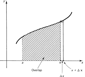
But since this is the difference between two partially overlapping ranges of integration (Figure 11.6-1), the result must be merely over the range that is not common to both, that is, x to x + Δx. (Remember that Δx can be either positive or negative.) Therefore, we have

If we think of f(t) as being a positive, continuous, monotone increasing function in this interval (decreasing makes trivial changes), then (going back to the sum definition of the integral) we have the bounds on the function in the interval Δx. If Δx is positive, then
Figure 11.6-1
lower bound = f(x) and upper bound = f(x +Δx)
where Δx is the length of the integration interval. Because f(x) is continuous, as Δx approaches 0 we have the same upper and lower bounds. And similarly for Δx negative. Thus we conclude that the derivative of the integral with respect to the upper limit of integration x is simply the function being integrated, the integrand. Be sure you see the inevitability of this result. Think about what is happening as the derivative of the integral is taken, how the rate of growth of the area under a continuous curve must be exactly the height of the curve at that point. The mathematics this time matches our intuition.
This is the fundamental theorem of the calculus,
![]()
(where a is some fixed value of x); the derivative with respect to the upper limit of the integral of a function is the function itself. Thus differentiation undoes integration. We see the truth of this in the integration of xk, Generalization 11.4-3. The integral with the upper limit x [use x in place of a in the formula (11.4-4)] is
![]()
Differentiating this with respect to x, we get the original integrand,
![]()
as the theorem requires. Thus integration is the inverse operation to differentiation, just as division is the inverse to multiplication. In both cases (division and integration), it comes down to a guess process. The question in integration is, “What function is this the derivative of?”
While the derivative of the integral is the original function, it is not true in general that the integral of the derivative of a function is the original function (the two operations do not “commute”). The reason for this is simple. Consider two functions that differ by a constant. Since the derivative of a constant is zero, their derivatives are the same. Therefore, given only the derivative, we cannot know which one was the original function. We know the integral only to within an additive constant; there is an arbitrary additive constant to be tacked onto the integration process when we think of integration as the antiderivative.
Example 11.6-1
Given that the derivative of a polynomial is
![]()
we find that the antidervative is (where C is some constant)
![]()
After some algebra, this is simply
![]()
You can always check an integration by differentiating the answer to recover the original expression.
Thinking about the matter (upper and lower sums, the limit, and the continuity in each interval), we see that the sum of two functions added together is the same as the sum of the two individual sums added together; integration is a linear operator, just as differentiation was.
![]()
We also see from the fundamental theorem of the calculus that since we can differentiate any powers, not only integral powers, we can also integrate them. It is convenient to write the formula for integration in terms of the antiderivative (any function whose derivative is the given function) of a single power of x as
![]()
for any n other than n = –1. We have deliberately omitted the limits of integration for the antiderivative, and have supplied the missing constant C that is arbitrary when we handle the antiderivative.
We clearly cannot do the case n = –1 using this formula, both because it requires a division by zero and because no differentiation of a power of x leads to the exponent –1. We will take up the problem of its integration in Chapter 14.
We need some notation. It is very convenient to write an antiderivative of f(x) as F(x). We have, therefore,
![]()
To get from the antiderivative to the integral between the limits of an interval, we merely note that the integral over an interval of no length
![]()
so that we must have for the special value x = a
![]()
From this we see that
C = −F(a)
or in general
![]()
where F(x) is any antiderivative of f(x). Notice how the additive constant C in the antiderivative F(x) disappears in the final result.
It is customary to call the antiderivative the indefinite integral, as contrasted with the integral with limits, which is called the definite integral.
Besides polynomials and sums of arbitrary powers of x (excluding n = –1), we can integrate many different expressions when we recall (Section 7.6) the function of a function formula for differentiation:
![]()
Example 11.6-2
What is the antiderivative of
![]()
We identify the u of formula (11.6-4) with
u = 1 + x2
Then the du/dx = 2x, and we have the form
![]()
![]()
It is always easy to check the antiderivative by the simple process of direct differentiation of the answer, and in this case we see that we have the correct antiderivative.
The constant of integration for the indefinite integral is not unique as the following example shows: one C is the other C + ![]() .
.
Example 11.6-3
Given the function to integrate
![]()
we can think of it as the sum of two terms and get the answer
![]()
or we can think of it in the form
u = x + 1
and get
![]()
We see that the letter C is not the same in the two cases.
Let us solve this same problem in the differential notation. We have
dy = (x + 1)dx
Upon integrating both sides, we get
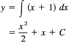
The result is, of course, the same.
The lack of uniqueness of the constant of integration can cause confusion for the beginner when the results obtained are not those in the book.
Example 11.6-4
What is the antiderivative of
![]()
We write this in the differential form
![]()
Again, how shall we pick the u? The radical is awkward, so we pick
u2 = 1 – x2
because this form will get rid of the radical. we get
![]()
We now have
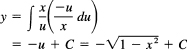
Differentiation confirms this result.
Example 11.6-5
Consider
![]()
We see that if we take the u = 1 + x4 then
du = 4x3 dx
If only we had an extra 4 to make the front term 4x3, we would have the proper du. Evidently, we merely multiply and divide by the 4 to get this. Thus we have, finally,
![]()
and this upon integration becomes
![]()
Differentiation verifies that we are right and indicates how the integration process reverses the differentiation steps.
There are no infallible rules for picking the substitution of a variable u for the original variable x. The fact is that the ability to chose a good substitution depends on your familiarity with the differentiation process; you must “see” how the verification by differentiation would go, how the terms would combine, cancel, and so on. If you are having trouble at this point, perhaps the best thing to do is practice some comparable differentiations until you have a feeling for how they go and can see how to make them go backward, beginning with the function, computing the derivative, and then imagine starting there and trying to reconstruct the original function. The differentiation process will show you, when you inspect it, exactly how to go backward as the integration process requires. It is probably much better to try a few problems and to carefully analyze what happens in each case, and why it happens, than it is to merely do a lot of problems with no careful examination of how the process goes. Familiarity is necessary so that you will learn to reverse the process of differentiation. Differentiation must be so automatic that you can see almost immediately how various choices will work out. In this, it is like factoring a quadratic such as
x2 – 4x – 12
You must see all the various factorings of 12 and select the one for which the difference of the factors is 4.
Furthermore, there is no unique way of doing an integration; there are often various substitutions all of which will work (but some may be easier than others). Finding the antiderivative is a guess process whose truth is easily verified by a final differentiation if there is any doubt in the correctness of the result. There is no excuse for accepting a result that does not differentiate back to the given derivative.
Example 11.6-6
Find the antiderivative of
![]()
This is the same as
![]()
We see the x4 under the radical and out in front the x3, which is what we need for the derivative of x4. Therefore, we pick the u as
u = 1 – x4
which leads to
du = −4x3 dx
We are lacking a –4, so we supply it, and compensate in the denominator to get
![]()
which integrates into
![]()
or
![]()
Rather than doing a long list of exercises, you are well advised, after doing a few, to make up your own exercises. At first, as we earlier suggested, you pick the function, differentiate it, and then imagine starting with the derivative to integrate. If you get stuck, then the differentiation process will show you exactly how to do the integration. Later, you should start with the function to integrate. This will require you to pick your problems with some care so that they can be integrated. In doing this, you will find more clearly exactly what is involved in the integrals you carl do. What evidence there is on the matter seems to show that your active involvement in the process teaches you more in less time than does the passive doing of problems that have been selected for you. As we have repeatedly said, we can only coach you; you must do the learning, and active participation in the learning process is generally much more effective than is passive following of what you are told to do. The best mathematicians generally find their own problems, work them out, and then go over them again and again, examining alternative strategies, until they have a sure mastery of the situation. There is an emotional involvement when you do your own problem that is usually missing when you merely do problems that others suggest.
Find the antiderivative of the following:
1. y′ = x3
2. y′ = x + x2 – x3
3. y′ = a + bx + cx2
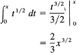
4. y′ = x1/2
5. y′ = 3 + x–1/2
6. y′ = c – ![]()
7. y′ = x3/2 – x1/2 + x-1/2
8. y′ = x(a2 + x2)4
9. y′ = ![]()
10. y′ = (x3 – x)3(3x – 1)
11. y′ = ![]()
12. y′ = ![]()
13. y′ = ![]()
14. y′ = ![]()
15. y′ = (a2 + x2)3(3x)
11.7 THE MEAN VALUE THEOREM
Before we go too far, it is necessary to examine the above argument closely. We glibly said that since the derivative of a constant was 0 it follows that all we have to do to get the general antiderivative is add an arbitrary constant C to any particular antiderivative we find. But are you certain that no function other than a constant can go into 0 when you differentiate?
The point is not trivial. The role of the additive constant in integration is central. You are claiming that when you differentiate then all functions differing only by a constant must go into the same function, and only those. You are claiming that there is no function other than a constant whose derivative is identically zero.
You need some kind of mathematical proof of this important observation. Given a function that is continuous in a closed interval a ≤ x ≤ b, denoted by [a, b], and that has a continuous derivative in the open interval a < x < b, denoted by (a, b), which is identically zero (in principle you cannot compute the derivative at the ends of the interval), then the function must be a constant. (A more complicated proof would not require the continuity of the derivative.) How to prove this kind of a statement is your problem.
Naturally, you begin by thinking about what you mean by a function being a constant. You mean that at any two points a and b (let them be the ends of the interval) you have
f(b) = f(a)
But you have learned from observation that it pays to try to prove not that two things are equal, but rather that their difference is zero. A trivial change in the problem, but one whose importance professional mathematicians well recognize. Therefore, the statement you want to prove is
f(b) – f(a) = 0
The statement you are given is
![]()
at all points in the interior of the interval. Can you equate these two expressions? No, the dimensions are wrong, the resulting equation would not be invariant under a scaling transformation; hence it would be a meaningless expression. The derivative is the quotient of the scaling factors for f(x) and for x, so you try
![]()
What value x? Certainly not all values! Is there at least one such x? If there is, then from knowing that the derivative is always 0 you would have the proof that the function is a constant, that f(b) = f(a).
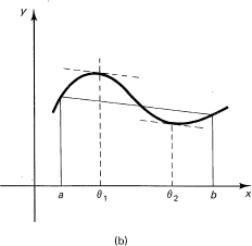
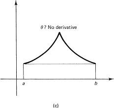
Some pictures of the situation are needed (see Figure 11.7-1). Yes, it does look as if it is a true statement and avoids the examples where there is a comer and hence no derivative at some point. The point where the equality holds is conventionally labeled by the Greek letter θ (lowercase theta).
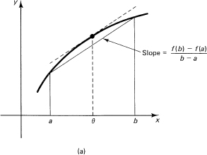
Mean Value Theorem. If a function f(x) is continuous in a closed interval [a, b] and has a continuous derivative in the open interval (a, b), then there is at least one value of x, labeled θ, such that
![]()
This theorem states geometrically that the slope of the secant line through the end points of the interval is equal to the slope of the curve for at least one interior point θ of the curve.
Can you simplify this theorem before you try to prove it? It seems that if you subtracted out the secant line through the end points you would have an easier theorem to prove. The secant line through the two end points is (it is a linear equation so you need only check this for x = a and x = b)
using the point-slope form (or two-point form if you prefer) of the line. Remove this line by subtracting it from the function. Now the theorem you want to prove is:
Rolle’s Theorem. If a function is continuous in the closed interval [a, b] and vanishes at both ends, and has a continuous derivative in the open interval (a, b), then there is at least one value of x, x = θ, such that
![]()
where a < θ < b.
Now look at the corresponding Figure 11.7-2. If you suppose that the function is positive in the interval, then when it first rises the derivative (slope or rate of change) is positive, and when the function returns to zero, as it must before or at the other end of the interval, the slope must be negative. Thus the derivative must change sign somewhere. But the derivative is assumed to be continuous, and recalling our assumptions about the existence of numbers, you recall (Section 4.4, Assumption 2) that there will exist a number where the function takes on the value 0. If there are several zeros of f(x) in the interval, then it suffices to use any one to show the existence of a place in the interval where the derivative is zero. If the function is negative, the argument is easily modified to fit this situation.

Figure 11.7-2
In the trivial case for f(x) = 0 for all values, it is easily seen that the derivative does vanish for at least one point in the interval.
From Rolle’s theorem you have the proof of the mean value theorem. And from that you get, via the assumption that the derivative was identically zero, that
f(b) – f(a) = 0
This says that any continuous function in a closed interval [a, b] whose derivative is continuous in the open interval (a, b) and is always zero must be a constant. There is no other admissible function, no matter how peculiar it may be, that meets the conditions. Therefore, it is sufficient to add the additive constant C to the antiderivative to get the most general function whose derivative is the given function.
You need, now, to examine the way you combined the individual pieces (each of which is a piecewise monotone continuous function) into the complete function over the whole range. First, there are only a finite number of such pieces. Second, there is a bit of trouble at the ends. At a discontinuity (see Figure 11.7-3) of the function you have the question of the value of the function. For example, suppose between
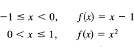
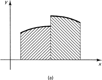
Figure 11.7-3
When you are working in the first interval and substitute in the upper limit of the range, x = 0, you want to use the value appropriate to the interval, that is,f(0) = –1, while for the lower limit of the second integral you naturally want to use f(0) = 0. Thus you want to have two distinct values of the function at the same place! This contradicts the claim of handling only single-valued functions. The trouble is clear; you should take the limits appropriate for each interval, but this requires a lot of words throughout the rest of the text. We leave it to the student to supply the limit arguments for handling this essentially trivial point.
We remind you again, the constant C need not be the same in various methods of integration of the same function, as shown in Example 11.6-3.
We proved the mean value theorem for functions with a continuous derivative in the open interval and remarked that a proof could be given with merely the assumption of a derivative in the open interval. The difference is so small that you do not often meet a function that has only the weaker condition and not the stronger, although such functions can be “made up.” We are generally concerned to handle the needs that arise in practice, and do not attempt to prove the weakest theorems we could.
EXERCISES 11.7
1. Prove Rolle’s theorem using only the existence of the derivative. Hint: Pick a point where the function takes on its extreme value in the closed interval. Argue that the difference quotient on one side must be ≥ 0 and on the other must be ≤ 0; hence, since the limit exists, the limit must be 0.
2. Using the function y = x(1 – x)2, show that in the interval [0, a] the corresponding value θ(a) is not a continuous function of a, for a as large as 3.
11.8 THE CAUCHY MEAN VALUE THEOREM
We will later need a generalization of the mean value theorem. It is probably best to deal with it now, because it uses the same kind of techniques we just used.
Consider two functions f(x) and g (x). We wish to prove that there exists a θ such that
![]()
supposing that both functions satisfy the same kinds of conditions that were needed in the mean value theorem, plus the condition that g(b) ≠ g(a). We cannot apply the mean value theorem to the numerator and denominator separately because then, in general, the two theta values would not be the same, as is asserted in the theorem we are to prove.
To apply Rolle’s theorem (which is the main tool), we construct the function
![]()
so that Φ(a) = Φ(b) = 0. We conclude that there is at least one point θ in the interval at which the derivative Φ′(x) vanishes. At this point we have
![]()
Now if g′(x) does not vanish in the interval, then we have
![]()
This is the extension we need. If g(x) = x, then this extension reduces to the original mean value theorem.
Cauchy Mean Value Theorem. If f(x) and g(x) are continuous in the closed interval [a, b] and have continuous derivatives in the open interval (a, b), and if g’(x) ≠ 0 [hence g(b) ≠ g(a)] in the interval, then
![]()
for some θ in the interval a < θ < b.
11.9 SOME APPLICATIONS OF THE INTEGRAL
At this point you can integrate comparatively few functions, so we must pick the problems carefully. Later, in Part III, you will greatly increase the class of functions you can integrate. We can, however, at this point give some flavor of the richness and variety of the applications of integration.
Example 11.9-1
Find the area under the curve
y = x – x3
between x = 0 and x = 1 (see Figure 11.9-1). You want the integral
![]()
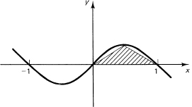
Figure 11.9-1
On the right-hand side, the bar at the end of the line corresponds to the earlier limits on the integral sign. From (11.6-3) we substitute the upper limit into the integrated function and subtract the value of it at the lower limit to get
Does the answer seem reasonable? The area of a triangle inside is x which is less than the computed area by about the right amount.
Example 11.9-2
Find the area under the curve
![]()
as a function of the upper limit (Figure 11.9-2). Remember to use a dummy variable of integration to avoid confusion with the upper limit x:
Is this reasonable? We can test it for x = 1. A bounding rectangle gives an area of 1, while an enclosed triangle gives an area of ![]() , and the triangle should be closer to the area, which is
, and the triangle should be closer to the area, which is ![]() ; and it is!
; and it is!
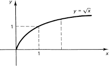
Figure 11.9-2
Example 11.9-3
Find the area under the curve
![]()
(see Figure 11.9-3) from the origin out to an arbitrary position x. You want the integral
![]()
This is not a simple power of t, so you need to think of what function of t you can call u(t). Some thought suggests trying u = a2 + t2 because you have
du = 2t dt
and there is already a t in the numerator. For the moment you lack the factor 2, so you put the 2 in the numerator and compensate by a factor ![]() out in front (for the same reason we could pass over constants when differentiating). You have, therefore,
out in front (for the same reason we could pass over constants when differentiating). You have, therefore,
Figure 11.9-3 ![]()
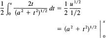
to be evaluated between the limits 0 and x. You get, finally, the area (upper limit t = x minus the lower limit t = 0):
![]()
A more suggestive way of writing this is
![]()
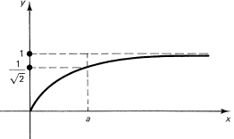
since this shows the answer in a form where x is related to the parameter a. In particular, at x = a you have the area
![]()
Does it seem to be a reasonable area? Look at the figure and estimate the area to check the answer. The enclosed triangle has an area of ![]() while the bounding rectangle has area of a/
while the bounding rectangle has area of a/![]() = (0.707 … a). All this suggests that in the original problem we should have set x = at and worked with the corresponding integral
= (0.707 … a). All this suggests that in the original problem we should have set x = at and worked with the corresponding integral ![]() .
.
Example 11.9-4
The number π. The transcendental number it arises in two ways: the circumference of a circle, C = 2πr, and the area of a circle, A = πr2. The first arises from the theorem that linear measurements of similar figures (circles in this case) are to each other as any other corresponding linear measurement (say radii). Thus
![]()
from which
C = 2πr
for some constant 2π.
For areas the theorem states that areas of similar figures are to each other as the squares of their corresponding linear measurements. Hence
A = πr2
Are these two occurrences of the symbol π the same number? To prove that they are, we divide the area of the circle into concentric rings of thickness Δri, (see Figure 11.9-4), choose any convenient radius ri in the ring of width Δri, form the sum
![]()
and finally take the proper limit to find
![]()
Thus the two occurrences of π are both the same number.
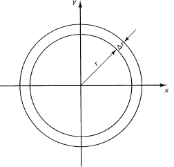
Figure 11.9-4 Area of a circle
Example 11.9-5
Find the formula for the volume of a cone. We think of the cone as upright with the vertex at the origin. The side that lies in the x–y plane would have the equation
![]()
where h is the height and r is the radius of the cone. We imagine the cone cut into horizontal slices of thickness Δy and radius x. The volume is, therefore,
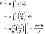
which is the known answer.
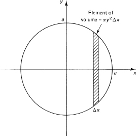
Suppose we rotate the parabola
y = x2
about the x-axis (see Figure 11.9-5). If we think of the fundamental process of integration, that is, the limit of a sum of terms, we see that the volume out to x = 1 can be approximated by a series of flat discs of radius y and thickness Δx. The element of volume is, therefore,
πy2Δx
We need no longer fill in all the details of upper and lower sums since clearly their difference will be bounded by the flat disc of maximum radius multiplied by the maximum thickness Δx, and in the limit the corresponding upper and lower sums will pass over to
![]()
But y = x2, so we have
![]()
as the volume. Does this answer seem reasonable? The volume of an enclosing cone would be π/3 (from Exercise 11.9-5). Yes, it seems reasonable.
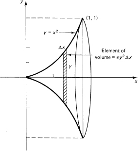
Figure 11.9-5 Parabola rotated about x-axis
Suppose we use the same parabola as in the previous problem except we rotate it about the _y-axis and ask for the corresponding volume. We note (Figure 11.9-6) how the shaded area is being rotated. Here the element of volume is the anchor ring whose inner radius is x and whose outer radius is 1. The element of volume is, therefore,
π(1 – x2)Δy
and the integral (remember we are integrating in the y direction and x2 = y)
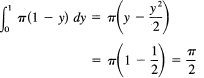
As a check, we could compute the volume of the inside and compare the sum of the two with the volume of the cylinder (see the exercises).
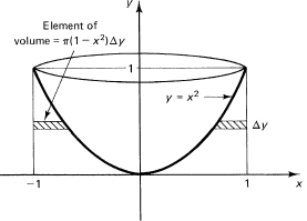
Figure 11.9-6 Parabola roated about y-axis
Example 11.9-8
Find the volume of a sphere of radius a. Draw a picture of a cross section (Figure 11.9-7)
The volume of a slice is
![]()
By symmetry, we have that the total volume is
![]()
which easily integrates into
![]()
as it should
Figure 11.9-7 Volume of a sphere by discs
Example 11.9-9
We have used discs to estimate the volume of a solid of revolution. Sometimes it is easier to use cylinders as the elements of volume (Figure 11.9-8). For the sphere in Example 11.9-8, we now have that the volume of the elementary cylinder is the surface, 2πrh, times the thickness Δx. Using only the upper half and doubling to get the total volume, we have
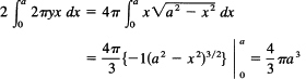
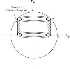
Figure 11.9-8 Volume of a sphere by cylinders
The use of a disc or a cylinder depends on the integration to be done; sometimes one is much easier to use than the other.
Example 11.9-10
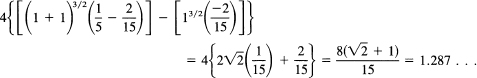
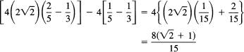
Just as we could differentiate identities to get new identities (Section 9.9), so too we can integrate them provided we watch the evaluation of the additive constant. For example, suppose you wanted the sum of
![]()
You could start with the basic generating function
![]()
and integrate it. Naturally, you integrate between t = 0 and t = 1. On the right you get the desired sum expression, and on the left you get, after the integration,
![]()
Putting in the limits, you get
![]()
as the desired sum.
Given the following function and limits compute the corresponding area:
1. y = x – x3, (0, 1)
2. y = x2 – x4 (0, 1)
3. y = 3x5 – 10x3 + 7x, (–1, 1)
4. y = 1 – ![]() , (0, 1)
, (0, 1)
5. y = 1/![]() , (1,4)
, (1,4)
6. y = x1/2 – x3/2 + x5/2, (0, 1)
7. y = ![]()
8. y = ![]() , (0, a)
, (0, a)
9. y = ![]()
Rotate the following curves about the x-axis and find the corresponding volume.
10. Exercise 1
11. Exercise 2
12. Exercise 4
14. Exercise 8
Rotate the following about the y-axis and find the corresponding volume.
15. Exercise 1
16. Exercise 2
17. Exercise 5
18. Exercise 4
19. Given the curve y = xn, for n > 0, and the interval (0, 1), (a) find the area under the curve and above the x-axis, (b) rotate about the x-axis, and (c) rotate about the y-axis.
20. Find the value of ![]()
21. Evaluate ![]()
11.10 INTEGRATION BY SUBSTITUTION
One of the two powerful methods of finding integrals of functions is substituting one variable for another, also called change of variables. We have used the method a number of times: It is based on the fundamental relation
![]()
which is the basis for much of differentiation; hence it is reasonable to believe that it could play a similar part in integration. For the purposes of integration, we prefer to write this in the differential form
![]()
when we change from the variable x to the variable t. Hence if x = g(t), then
![]()
We often use this in the reverse direction; we recognize that we have some function of a variable multiplied by the derivative of that variable.
Example 11.10-1
Suppose you have the indefinite integral
![]()
If you set
1 + x2 = t
then using the differential notation you have
2x dx = dt
and in the t variable you have
![]()
Differentiation will convince you that this is the right answer.
The careful student may worry about the substitution
1 + x2 = t
being multiple valued. You have only to think of the substitution as a notational change and in each appearance of t write 1 + x2 to see that the result is safe at this step. You do need to think about the point when you substitute in the two limits.
Case Study 11.10-2
Find the indefinite integral
![]()
Even the experienced person finds it difficult to imagine what function would differentiate into this integrand, ![]() .
.
Square roots are generally awkward to handle, so the most obvious substitution is
x = u2
dx = 2udu
Therefore, the integral is
![]()
which shows some progress in making the integrand more tractable. To get rid of the remaining square root, we next try
1 + u = v2
du = 2v dv
and we have
![]()
This integral is easy to do. We get
![]()
It remains to substitute back twice, once to get from v to w, and then to go from u to get to the original x variable. We have first
Finally, going back to the x variable we get
![]()
as the indefinite integral. This can also be written in the form
![]()
Direct differentiation will show that this is the correct answer. Of course, now that we have the result we see that the two substitutions could be combined into one change of variable
x = [v2 – 1]2
This is the typical polishing up mathematicians do when presenting the final result; and if you can see far enough ahead, you can likewise do the integral with one substitution.
Example 11.10-3
In the previous case study, suppose we had been asked for the definite integral
![]()
Using the answer, we merely put in the limits to get
A sketch of the integrand shows that it lies between 1 and ![]() so that the answer must lie there too.
so that the answer must lie there too.
However, had we started with the definite integral problem there is another approach. Once we made each substitution, we could have also brought the limits of the integral to the new variable, and thus saved all the back substitution to get back to the variable x. The start would have been
![]()
The substitution
x = u2
moves the limits in the variable x from 0 to 1 to the same range 0 to 1 for the variable u, so we have
![]()
The substitution
1 + u = v2
moves the limits 0 to 1 in u to the range 1 to ![]() in the variable v, so we have
in the variable v, so we have
![]()
whose integration gives, as before,
![]()
and substituting in the limits we get
as before. A comparison shows that probably in this case the moving of the limits to the new variables is preferable to transforming the variables back to the old limits. Sometimes it is easier to do the back substitution of the variables; there is no fixed rule in this matter.
Integrate the following:
1. ![]()
2. ![]()
3. ![]()
4. ![]()
5. ![]()
6. ![]()
7. ![]()
8. Show that for any integrable function f(x)
![]()
Hint: Substitute a – x = t and combine with original integral
10. Show that ![]()
11. Show that ![]()
12. Show that ![]()
13. Show that ![]()
14. Show that for ![]()
11.11 NUMERICAL INTEGRATION
Many integrals that naturally arise cannot be integrated in any finite form in terms of commonly used functions (cannot in the same sense that ![]() ≠ p/q, and not in the sense of ignorance). Still, you believe that the corresponding problem, when presented as an area, has some definite value. Thus, when all other integration methods fail, numerical integration is used to estimate the corresponding area. If the integral involves one or more parameters, you try to eliminate them by suitable scale transformations, and if this does not work, then you face the numerical evaluation for each parameter value of interest.
≠ p/q, and not in the sense of ignorance). Still, you believe that the corresponding problem, when presented as an area, has some definite value. Thus, when all other integration methods fail, numerical integration is used to estimate the corresponding area. If the integral involves one or more parameters, you try to eliminate them by suitable scale transformations, and if this does not work, then you face the numerical evaluation for each parameter value of interest.
For example, given the integral
![]()
the substitution x = at gives
![]()
and we have an integral free of the parameter a.
The central idea behind numerical integration is analytic substitution: for the function you cannot handle, you approximate it locally by one you can handle. This is the same idea that is behind Newton’s method (Section 9.7, where you replaced, locally, the curve by the tangent line, and then found the zero of the tangent line as a new approximation to the zero of the function.
Given
![]()
suppose we approximate f(x) by a straight line through the two end points, that we approximate the area by a trapezoid. The approximation to the function is the line
![]()
That this is the desired line can be seen from the fact that it passes through the two points (0, f(0)) and (1, f(l)). We therefore integrate this approximation as if it were the function
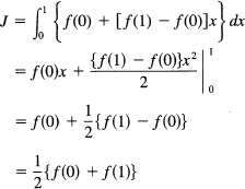
which is the known area of a trapezoid (see Figure 11.11-1).
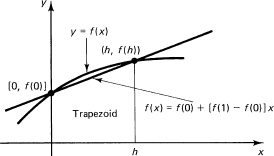
Figure 11.11-1 Trapezoid area
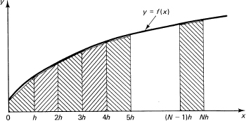
This is a crude approximation to the function, and you promptly think of breaking up the interval [0, 1] into, say, N subintervals, and then using this same trapezoid approximation in each interval (see Figure 11.11-2). The fact that the integral was defined to be the limit of a sum suggests inverting this definition and estimating the integral as a sum of small elements. If we write h = 1/N, then we have for an estimate of the area J the composite trapezoid rule
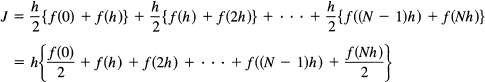
It is easy to generalize to an arbitrary interval (a, b). Again using N subintervals, we have
Figure 11.11-2 Trapezoid rule
![]()
where h = (b – a)/N. In words, the area estimate for the trapezoid rule is the sum of all the equally spaced N + 1 integrand values except that the first and last have coefficients ![]() and the whole sum is multiplied by the length of a subinterval (b – a)/N.
and the whole sum is multiplied by the length of a subinterval (b – a)/N.
It can be shown that the error in the interval can be expressed by
![]()
(for some θ in the interval), and hence for the whole interval
![]()
(although the complete proof is not easy). Thus we have the following rule: halving the interval reduces the trapezoid rule error by a factor of 4.
An alternative approximation, still using straight lines, is the midpoint formula. We again divide the interval [a, b] into N subintervals, but this time we use the tangent line at the midpoint of the interval. From the Figure 11.11-3 we see that by tilting the tangent line until it is horizontal the area under it in the subinterval will not change. The composite midpoint formula is, therefore,
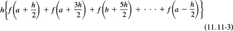
It is simply the sum of the samples of the function taken at the midpoints of each interval multiplied by the length of a subinterval.
It can be shown (and you can see that it is approximately true from Figure 11.11-4) that the error per interval is half that of the trapezoid rule and with the opposite sign:
![]()
Therefore, the total error is approximately
![]()
We see that the midpoint formula has approximately half the error as the trapezoid rule, has simpler coefficients, and requires one less evaluation of the function. Furthermore, the error is of the opposite sign.
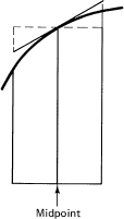
Figure 11.11-3 Mid-point integration

Figure 11.11-4 Comparison of errors
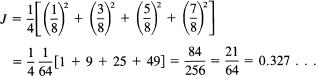
Example 11.11-1
As a check case we find the area of a known value
![]()
Let us take N = 4 so that we can follow the arithmetic easily. The trapezoid rule gives
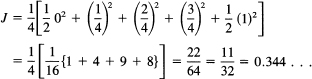
The midpoint formula gives
The true answer is, of course, ![]() , and the errors are
, and the errors are
trapezoid error = 0.011
midpoint error = –0.006
and, as predicted, the midpoint has half the error and the error is of the opposite sign. The error formulas could be used to estimate the error since the second derivative is exactly 2 for all θ.
To get more accuracy, you could take many more intervals (N much larger), but that involves more arithmetic, and leads in extreme cases to increased roundoff error in the arithmetic done. Instead, there is an alternative approach to get more accuracy. We could use a better local approximation to the function than straight lines. Thus we next look at local parabolas through three equally spaced points.
To find the formula for a parabola through three equally spaced points, we use the method of undetermined coefficients. Let the given x values be -h, 0, and h. For the function we have
y = A + Bx + Cx2
and we have the three equations (see Figure 11.11-5)
f(-h) = A – Bh + Ch2
f(0) = A
f(h) = A + Bh + Ch2
We get as solutions
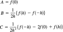
The integral from −h to h of this parabola is
![]()
and substituting in the values of the coefficients we get, after some algebra,
![]()
To convert this into a composite formula, we note that translating a parabola does not change the quadratic nature of the curve; hence the same formula applies after translation. The composite formula, when you note that the ends of each interval (except the very first and last) occur twice, is
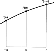
Figure 11.11-5 Derivation of Simpson’s formula
![]()
For the inner points, the odd numbered get weight 4 and the even ones get weight 2, while the end ones get weight 1. The pattern of weights is
![]()
The error term of the composite formula has the form
![]()
Notice that this formula is exact for cubics, although we only started with quadratics in our approximation. The reason is easy to see from Figure 11.11-6, where we see that the cubic has a canceling error in the double interval. This formula is called Simpson’s formula, is exact for cubics, and requires an even number of subintervals.
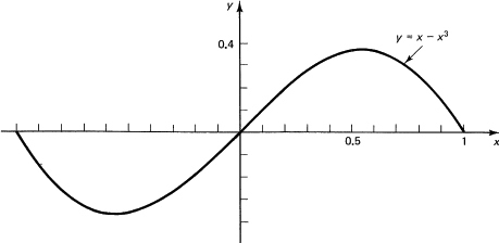
Figure 11.11-6 Typical cubic
As a check on Simpson’s formula, suppose we apply it to a cubic
y = x3
from 0 to 1. We pick N = 2, meaning four subintervals, and h = ![]()
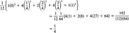
which is the correct answer.
Example 11.11-3
Suppose we use the known integral (which at present you cannot integrate)
![]()
We will again use Simpson’s formula with a crude spacing, N = 2 (meaning four intervals, h = ![]() ). We have the table
). We have the table
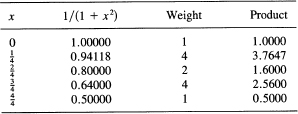
The sum is 9.4247, and this is to be multiplied by h/3 = ![]() . The result is
. The result is
Simpson = 0.78539
true = 0.78540
which is remarkably close.
We have given only three of an almost infinite number of numerical integration formulas. Each may be programmed as a process, even on a small programmable hand calculator, with the particular function left as a subroutine to be supplied by the user in the specific case. The calling sequence gives the range numbers a and b, the number of intervals N, and the name (or location) of the description of the function to be integrated. Thus, these formulas are general methods of wide applicability once you have written the basic program. Unquestionably, Simpson’s method is the most widely used in practice. The other two are inferior for most functions (but there are functions where the midpoint formula gives a better answer). You can see how you could derive many other integration formulas if you wished; simply find another approximation method and integrate it. Given noisy data, for example, you might choose to fit by least squares.
EXERCISES 11.11
Compute the following areas using the indicated methods:
1. (1 + x3)1/2, (0, 1), trapezoid and midpoint, N = 4.
2. (1/x), (1, 2), trapezoid and midpoint, N = 6.
3. 1/x, (1, 2) Simpson, N = 3
4. 1/(1 + x2), (0, 1) trapezoid and midpoint, N = 4
5. 1/(a2 + x2), (0, a), reduce to computable form
6. 1/x2, (1, ∞), midpoint, any N you want
11.12 SUMMARY
We introduced the idea of an integral as a limiting method for finding areas of regions with curved edges. For continuous functions, the upper and lower sums were found to converge to the same limit as the largest interval size approached zero. The idea of area was then generalized to be the limit of any sum of elements, including discs, rings, and cylinders, or any other regular shapes.
We proved the fundamental theorem of the calculus, that the derivative of the integral is the integrand. This is the tool we use to find areas; we find an antiderivative (the indefinite integral) of the integrand and then substitute in the limits of integration.
Not only did we find various limits of sums; we also used the operation of integration to find new identities from old ones.
Finally, we looked briefly at the problem of what you can do when you cannot integrate the given function in terms of known functions. We gave three methods of integration, although there are many others. Day in and day out it is Simpson’s formula that is used more than all others put together.