16.1 REVIEW OF THE TRIGONOMETRIC FUNCTIONS
We first review the trigonometric functions carefully because we are going to use them extensively in the calculus. It is necessary for you to overleam the many relationships between these functions so that in the middle of doing a calculus problem you are not distracted by the inability to recall easily the needed information. You are advised to learn by rote the many things that are reviewed here (remember the usefulness of flash cards). There is no royal road to mathematics, and the longer you delay in mastering the details the longer you will be held up in learning to use the calculus and probability.
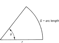
The first novelty is that in the calculus we always use the radian measure of angles; it is the natural measure to use in the calculus. Radian measure is usually defined as the ratio of the length of the arc of the circle, centered at the vertex of the angle, to the length of the radius (see Figure 16.1-1). We have, therefore,
![]()
Thus the radian measure of an angle is a pure, dimensionless number (a dimensionless number does not depend on the units used). Since the circumference of a circle is 2πr, we have that 360° corresponds to 2π radians. One radian is clearly 180°/π = 57.295779 … °, and one degree is π/180 = 0.017543 … radians.
Trigonometry rests on the theorem in geometry that similar triangles have the same ratios of corresponding sides (Figure 16.1-2). Consequently, the ratio of any two
Figure 16.1-1 Angle in radian measure
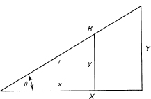
Figure 16.1-2 Similar triangles
sides of a triangle does not depend on the size of the triangle but only on the shape. Trigonometry is further simplified by tabulating only the ratios for right triangles. The six possible ratios (dimensionless numbers) for right triangles are defined by Figure 16.1-3.
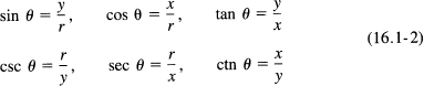
The second line is simply the reciprocal of the first line. The “co” in the cofunction means “any function of π/2 – θ (the complementary angle) is the cofunction.” Thus sine and cosine are each the complementary function of the other. The sine, cosecant, tangent and cotangent are all odd functions, meaning that f(–θ) = –f(θ). The other two, cosine and secant, are even functions, meaning f(–θ) = f(θ).
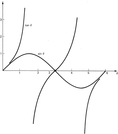
Next, the idea of an angle is extended to any size. Figure 16.1-4 shows the angle in the second quadrant. Any real number, positive, negative, or zero, no matter how big or small, can be an angle. The corresponding graphs of the trigonometric functions are periodic with period 2π (or shorter)(see Figure 16.1-5). You have only to imagine the angle increasing at a constant rate, and imagine the corresponding ratio as time goes on, to see why the graphs appear as they do.
Certain angles occur repeatedly, and corresponding values of the trigonometric functions should be learned. At 0 and π/2 the values are obvious from their graphs, and we have written “∞” when we have a division by 0. The other angles arise from special triangles. For π/4 you have the 45° triangle (Figure 16.1-6) with both sides
Figure 16.1-3 Basic triangle
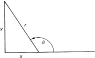
Figure 16.1-4 Extension of angle
Figure 16.1-5 Sin θ and tan θ
equal to 1 and the hypotenuse equal to ![]() . The other special triangle is the 30°–60° triangle with one side equal to 2; it arises from bisecting one angle of an equilateral triangle of side equal to 2 (Figure 16.1-7). The angles are, in radian measure, π/6 and π/3. We thus have the Table 16.1-1
. The other special triangle is the 30°–60° triangle with one side equal to 2; it arises from bisecting one angle of an equilateral triangle of side equal to 2 (Figure 16.1-7). The angles are, in radian measure, π/6 and π/3. We thus have the Table 16.1-1
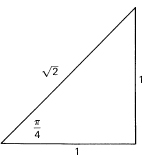
Figure 16.1-6
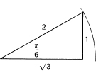
Figure 16.1-7
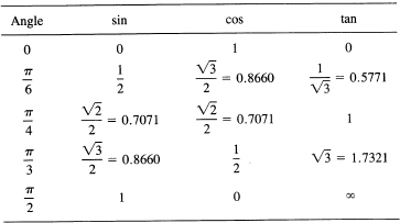
One easy way to remember these numbers is to note that the entries in the sine column are ![]() .
.
Next come the identities among the different functions. The circle, which we imagine the point (x, y) running around, has the equation
x2 + y2 = r2
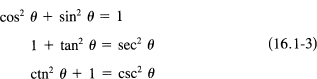
Divide this equation in turn by r2, x2, and y2 to get, using (16.1-2), the three basic identities:
To handle the solution of triangles, we draw a typical (obtuse) triangle in Cartesian coordinates (see Figure 16.1-8). If we apply Pythagoras’s theorem to the corresponding right triangle, we get (in the figure x is negative)
(a – x)2 + y2 = c2
Expand the binomial and recall that
x = b cos C and y = b sin C
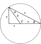
Figure 16.1-8
![]()
Using sin2 C + cos2 C = 1 (16.1-3), we get the law of cosines:
![]()
Note that if C = π/2 then cos C = 0, and you have the Pythagorean theorem as a special case of the law of cosines.
The law of sines is derived by dropping a suitable perpendicular in the general triangle and then expressing this distance as the sine of the opposite angles (see Figure 16.1-9). Eliminating h, we have
![]()
from which, by symmetry, it follows that this is also equal to (sin B)/b.
To get the addition formulas of trigonometry, we consider Figure 16.1-10. For convenience, we pick a unit circle. We first compute the length of the side PQ = z. We have
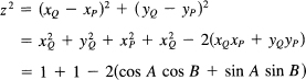
If we apply the law of cosines to this same triangle with side z, we have a second expression for the same thing:
![]()
Equating these two expressions, we find, after some algebra, that
![]()
This is one of the four addition formulas for the sum and difference of two angles.
To get the next addition formula, merely change (since the identity is true for all angles) B to – B, and remember that cos (–B) = cos B, while sin (–B) = –sin B. We get

Figure 16.1-9
Figure 16.1-10
![]()
Next, in (16.1-6), replace B by π/2 – B. We get (on interchanging the order of the terms and using the complementary angle)
![]()
In this formula we replace B by —B to get the last of the four addition formulas:
![]()
The double-angle formulas follow easily by putting A = B in (16.1-8) and (16.1-7):
In (16.1-11), write A/2 in place of A, and solve for the sine and cosine to get the half-angle formulas:
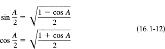
where, of course, you need to be careful as to which quadrant you are in since we have neglected to attach the ± sign to the radicals.
To get the sum formulas, we first add (16.1-8) and (16.1-9):
![]()
Now change variables by setting
A + B = x
A – B = y
Solve these equations for A and B:
![]()
And substitute into Equation (16.1-13):
![]()
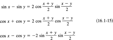
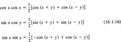
Finally, the product formulas are found from (16.1-6), (16.1-7), (16.1-8), and (16.1-9) by suitable additions and subtractions:
A useful formula for tan (A ± B) can be found as follows:

Now divide both numerator and denominator by cos A cos B to convert terms to tangents.
![]()
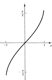
The inverse trigonometric functions are widely used in the calculus and require examination. From Section 15.1, we see the necessity for defining the inverse function so that only one value arises, called the principal value. An examination of the sine curve shows that it goes from —1 to +1 as the angle goes from —π/2 to π/2. The inverse function of the sine is sometimes written as
![]()
but this notation can be confused with (sin x)−1 = 1/sin x, and therefore we will always use the safer notation
Arcsin x
Figure 16.1-11 Arcsin x
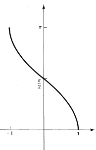
Figure 16.1-12 Arccos x
to mean the inverse function (Figure 16.1-11), and use
Arcsin x
to mean the principal value.
Correspondingly, we need an Arccos x function. The interval in which the cosine covers the full range only once is conveniently chosen as the interval from 0 to π. Finally, for the Arctan x we have the interval – π/2 to π/2. The sketches are shown in Figures 16.1-12 for the Arccos x and 16.1-13 for the Arctan x.
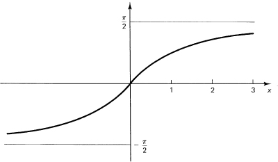
Figure 16.1-13 Arctan x
Before we take up the differentiation of the trogonometric functions, we develop a special limit
![]()
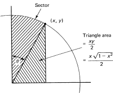
To prove this formula, we can use the area rather than the circumference (since from Example 11.9-4 they are somewhat equivalent). We look at Figure 16.2-1 and compare the three areas, the area of the inner triangle, the area of the sector of the circle, and the area of the outer triangle. These areas are
![]()
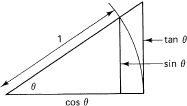
Figure 16.2-1 A particular limit
The area θ/2 of the sector follows from the symmetry of the circle plus the fact that the area of the circle is π while the central angle is 2π radians. For the moment, consider only θ >0 to get
![]()
Now take the reciprocals of each term (thus reversing the inequalities):
![]()
Finally, as θ →0+, both end terms approach 1; hence, by continuity, the quantity between them must also approach 1. The proof is for positive θ; but if θ is replaced by − θ then (sin −θ)/(−θ) = (sin θ)/θ, and the proof goes much the same.
This limit depends crucially on the use of radian measure for the angle and is the reason we use radian measure throughout higher mathematics.
16.3 THE DERIVATIVE OF SIN x
To find the derivative of y = sin x, we go back to fundamentals, to the four-step delta process (Section 7.5). At the third step, we have
![]()
We apply the top trigonometric identity of (16.1-15) for the difference of the two sines to get (note the 2 in the denominator of the denominator)
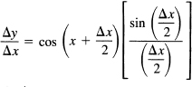
As Δx→0, so also does Δx/2→0 , and the limit of the term on the right is 1 [from 16.2-1)]. At the same time, x + Δx/2→ x. In the limit we have
![]()
One crude way to see the truth of this is to inspect the slope of the sine curve at each x value; the slope of the sine curve is the value of the cosine curve at the same x value for all x!
More generally, we have
![]()
Examples 16.3-1
We have (sight differentiation)
16.4* AN ALTERNATIVE DERIVATION
We found in Section 14.3 the derivative of the In x function by considering it as an integral, and later in Section 14.4 used the direct delta process. It is natural to ask if we need to apply the direct delta process [which used the special limit of (sin θ)/θ of Section 16.2] in order to find the derivative of sin x. Could we not find it, as we did for the In x function, by some method, perhaps directly from the integral? The answer is yes, as the following shows.
Consider finding the area in Figure 16.4-1. It is
![]()
Figure 16.4-1 Alternative derivation
Using for convenience the unit circle
x2 + y2 = 1
the integral becomes (note the dummy variable t)
![]()
Integrate by parts, choosing
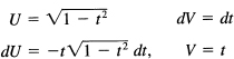
Hence
![]()
The integrand of the second integral can be written as
![]()
The original integral can now be written
![]()
Solve for J:
![]()
The integrated term is exactly the area of the triangle, and hence the integral on the right is the area θ/2 of the sector. We have (upon doubling each side of the equation)
![]()
From the fundamental theorem of the calculus, the derivative of the integral is the integrand:
![]()
This in turn means that, since from the figure x = sin 0, the radical is cos θ, and we have
![]()
(in the first quadrant). We have the derivative of sin θ is cos θ (without having used the limit of Section 16.2). The extension to the other quadrants follows easily from the addition formulas.
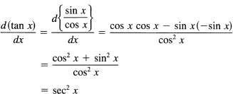
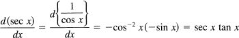
16.5 DERIVATIVES OF THE OTHER TRIGONOMETRIC FUNCTIONS
The derivatives of the other trigonometric functions follow immediately. For the function cos x, once you remember that
![]()
you have
![]()
Using these,
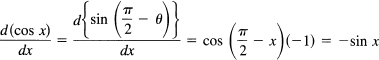
where the cofunction rule is applied again in the last step.
The derivative of the tangent is (using the quotient form)
The derivative of the secant follows from
The other two derivatives can be found directly or from the cofunction relationship. In the later case you replace each function by its cofunction and add a minus sign (coming from the differentiation of the π/2 – θ) to the result. You get the formulas
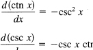
Thus we have the six basic formulas
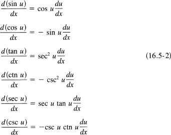
These formulas should be memorized carefully so they are available for immediate recall when we get to the topic of integration.
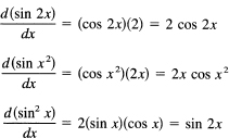
Example 16.5-1
Sight differentiate
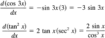
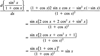
This surprising result comes from not first simplifying the expression before differentiation. If you simplify first, then instead of the above mess of algebra and trigonometry you have
Differentiate the following;
1. cos 2x, cos x2, cos2x
2. tan2x
3. sec2x
Check the following identities by differentiating both sides and comparing the results.
4. sin2x + cos2x = 1
5. 1 + tan2x = sec2x
6. ctn2x + 1 = csc2 x
7. sin (a + x) = sin a cos x + cos a sin x
8. cos (a + x) = cos a cos x – sin a sin x
9. sin x = tan x(cos x)
10. sin 2x = 2 sin x cos x
11. cos 2x = cos2x − sin2x
12. tan 2x = (2 tan x)/(1 − tan2x)
Find the derivatives of the following
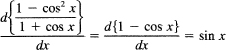
13. sin x/(1 + cos x)
14. (1 + cos x)/sin x
15. (1 + sin x)
16. tan x sec x
17. ctn x ctn x
18. (1 – sin x)/(1 + sin x)
19. (1 – cos x)/(1 + cos x)
20. tan2x – sec2x
16.6 INTEGRATION FORMULAS
The six differentiation formulas lead directly to the following integration formulas:
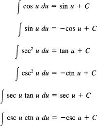
It is natural to wonder about the missing formulas, such as
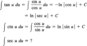
For the integral of secx, we need to know a trick (which was not easy to find the first time). Multiply and divide by the same quantity sec u + tan u:
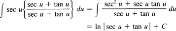
Correspondingly,
![]()
From these basic formulas for integration, we can find numerous other integrals. The main tools are as follows:
1. Rearrangement of the integrand (in these cases this means extensive use of the trigonometric identities of Section 16.1).
2. Recognition of a basic formula in some disguise. For example,
![]()
Set U = sin x, then dU = cos x dx, and the integral has the form
![]()
When used systematically, this becomes change of variables of Section 11.9.
3. Integration by parts, Section 14.7, which is very powerful, especially in getting rid of undesired terms.
4. Change of variables is mainly a matter of trial and error. It is often the only practical approach to difficult integrals.
As the following examples show, these tools can be combined in many ways to accomplish an integration. The examples also show that integration is a complex, difficult art that requires your best efforts. Each example of integration you do should be carefully studied so you gradually learn the art of integration; examine your successes as well as your failures! Ask yourself what other integrals could you do using the same method (or a similar method)?
Example 16.6-1
∫ cos 3x dx. You see immediately that 3x is the U, so that dU is 3 dx and you need a factor 3. Thus you get
![]()
Similar integrals are cos ax, cos (ax + b), and sin (ax + b). Do these in your head.
∫ sin2 x dx. Here you use the trigonometric identity for the half-angles (16.1-12) applied to the angle x:
![]()
Hence

Differentiation will show how the terms combine to reverse the steps you used. Evidently, cos2 x could be done in a similar way.
Example 16.6-3
∫ cos3 x dx. Here you need to see that cos2 x = 1 − sin2 x. Hence
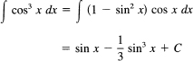
The integral of sin3 x would be similar. Integrals with odd powers of either sin or cos could be done similarly.
Example 16.6-4
∫ tan2 x dx. Here you need to notice that tan2 x = sec2 x − 1 and that sec2 x is the derivative of tan x. Hence you have
![]()
How about ctn2 x?
Example 16.6-5
∫ x sin x dx. Clearly, the trouble is in the factor x, and to get rid of it calls for integration by parts.
![]()
Hence

Direct differentiation will serve to check this result. Similar integrals are x cos x and x2 sin x.
Example 16.6-6
∫ sin x/(1 + cos x) dx. You need to notice that (except for the sign) the numerator is the derivative of the denominator. Hence
![]()
Absolute values are not needed in this example.
Example 16.6-7
J = ∫ e-ax sin bx dx. This integral occurs frequently and requires integration by parts twice, which will make the same integrand appear again. It does not matter which way we pick the U and dV. We pick
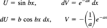
Hence
![]()
We apply integration by parts again, keeping the same order (lest we merely undo the step we just did):
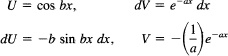
![]()
Notice that the original integral J has reappeared. Multiply by a2, and clean up the expression a bit:
![]()
Transpose the b2J term and solve for J:
![]()
Differentiation will verify this integral. The integral of e —ax cos bx would go much the same.
![]()
∫ sec3 x dx. This is even more complex than the last one, but again it is one of common occurrence. After a number of fruitless trigonometric substitutions, you will hit upon trying sec2 x = 1 + tan2 x.
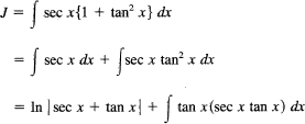
Apply integration by parts to this integral:
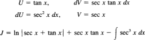
and the integral is J again. Solve for J and get
![]()
Again, differentiation will check this integration. Note that the device of getting the original integral back again and solving for it has occurred three times. This indicates that it is more than an isolated trick.
Example 16.6-9
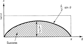
Buffon’s needle. Buffon (1707–1788), a French naturalist, suggested the following Monte Carlo determination of π. Imagine a flat plane ruled with parallel lines having unit spacing. Drop at random a needle of length L < 1 on the plane. What is the probability of the needle crossing a line?
“At random” will be taken to mean that the center of the needle is uniformly spaced from the nearest line. It is no loss in generality to assume that it lies on the positive side, 0 ≤ x ≤ 1/2. We also assume that the angle the needle makes with the line, θ, is uniform, 0 ≤ θ ≤ π (Figure 16.6-1). A crossing occurs (see Figure 16.6-2) when the coordinates fall in the shaded region of the sample space. The bounding line between the two regions, success and failure, is
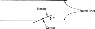
Figure 16.6-1 Buffon’s needle
Figure 16.6-2 Buffon’s needle
![]()
The probability assignment is uniform in the sample space. Thus the probability of acrossing is the ratio of the shaded region to the whole sample space. The area of the shaded space is
![]()
The area of the whole space is (1/2)π = π/2. Hence the probability of a crossing is
![]()
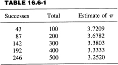
Again, we have a Monte Carlo method of estimating the known number π. As a test, we chose L = 0.8 and ran the cases as shown in Table 16.6-1. Thus the estimate of π is given by
![]()
We notice that the first 100 trials were not close to the correct answer, but the following trials are gradually “swamping” the first unlikely run.
Integrate the following:
1. ∫ sin (ax + b)dx
2. ∫ cos2 xdx
4. ∫ ctn2 xdx
5. ∫ x2 sin xdx
6. ∫ ![]() cos2 xdx
cos2 xdx
7. ∫ sec2 x/(1 + tan x)dx
8. ∫ eax cos bx dx
9. ∫ csc3 xdx
10. Show that ![]() 1/(1 + ex)dx = ln 2.
1/(1 + ex)dx = ln 2.
11. Integrate ∫ sec x tan x/(1 + sex x)dx.
12. Derive the integral for csc x.
13. Generalize Exercise 5 and get a reduction formula for it.
14. Do the Buffon needle problem in case L = 1.
15. Analyze the Buffon needle problem in case L > 1.
16. You are on a river bank. You walk in a random direction away from the river for one mile. At this point, you choose a new random direction and start walking another mile. What is the probability you will reach the river?
16.7 SOME DEFINITE INTEGRALS OF IMPORTANCE
Definite integrals are usually found from the corresponding indefinite integrals. In the process of substituting in the limits, often the integrated term will vanish at either or both ends, thus making the final formula much simpler.
Example 16.7-1
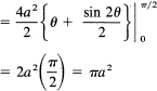
In Section 11.3, we said that we would later find the area of a circle. We found the area in Example 11.9-4, but we will do it again by a different method. Let the circle be defined by
![]()
The area is four times the area of one quadrant
![]()
Set x = a sin θ; then dx = a cos θ dθ, and we have
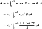
which is the correct answer.
Example 16.7-2
The Wallis (1616–1703) integrals occur so often in practice that they are worth special attention. They are
![]()
where n is a nonnegative integer. The equality of the two integrals is immediately obvious from their graphs (or else you can set x = π /2 − x′ to get the cofunction, the interchange of the limits, and the minus sign from the differentiation). We plan to first get a reduction formula for Wn. We write, for n ≥ 2,
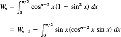
Apply integration by parts:
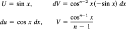
Hence
![]()
The integrated piece vanishes at both ends since n > 2, Multiply through by n − 1,
![]()
and solve for Wn.
![]()
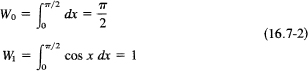
which is the required reduction formula. Each application of the formula reduces the index n by 2. To complete the cases, we need to compute the two bottom ones, n = 0 and n = 1. We have
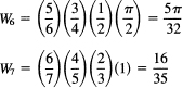
For example, repeated use of (16.7-1) ending with one application of (16.7-2) gives
Rule. To write out the answer, you begin with n in the denominator, n − 1 in the numerator, n − 2 in the denominator, n − 3 in the numerator,…., until you are down to 2. If the 2 ends in the denominator, you include a factor π/2, and if the 2 ends in the numerator you are done.
It is slightly more complex to handle the generalized Wallis integrals of the form
![]()
but corresponding reduction formulas for either exponent can be found by the same method. As you can see, there are no new ideas involved, only a great deal more tedious algebra.
Reduction formulas are similar to mathematical induction downward; therefore, it is not surprising that reduction formulas play a prominent role in dealing with classes of formulas.
Example 16.7-3
Stirling’s formula again. In Section 15.4 we found bounds on n!:
![]()
We asserted that for large n the proper coefficient of the approximation is
![]()
To find this coefficient, we use the Wallis integral. First notice that |cos x| ≤ 1. Therefore, for the range 0 ≤ x ≤ π/2,
![]()
Hence the Wallis integrals have the same relationship:
![]()
Divide by w2n-1. We get
![]()
We now use the rule for the Wallis integrals. This gives
![]()
Rearranging this we can write it in the form (where we supply a needed factor 2nn in the numerator and denominator)
If we take the positive square root of each term, we preserve the inequalities. We next insert in the numerator and denominator of the middle term a copy of the denominator. This gives
![]()
Write Stirling’s approximation in the form (with the coefficient C undetermined)
![]()
We substitute this into each appearance of a factorial in (16.7-3). This gives
![]()
Almost everything cancels out to leave
![]()
Now as n → ∞ the quantity in the middle is squeezed toward 1; hence
![]()
as we asserted.
Numerous other definite integrals occur in practice and are worth looking at.
Example 16.7-4
Probably the most common definite integrals are
The proofs are all the same in the sense that they are based on the same group of trigonometric identities (16.1-16). For the top integral, we use
![]()
The integration of this gives, if m ≠ n,
and at the two ends both terms vanish, being sines of multiples of 2π. For the case m = n ≠ 0, the second term will be cos 0x = 1, which integrates into an x. The limits and the 1/2 in front combine to give just π. In the final case, when both m = n = 0, the original integrand is simply 1 and the integral is, of course, 2π. The other two integrals may be found similarly, something that the reader should do.
Example 16.7-5
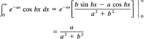
The integral for a > 0
![]()
Its indefinite integral is given in Example 16.6-7. Hence
![]()
and it is a matter of substituting in the limits. At the upper limit, ∞, the exponential dominates everything and gives 0. At the lower limit the sine vanishes and the cosine is 1; so we have
![]()
Similarly (for a > 0),
Example 16.7-6
Another definite integral of common occurrence is
![]()
for n a positive integer. Integration by parts (when n ≥ 2), using one x for the integration of the exponential and the resulting xn–1 for the U, gives
![]()
The integrated part vanishes at both limits since the exponential dominates any power of x. Thus you have the reduction formula
![]()
The index drops by two each step, and as a result you need the two bottom cases, n = 0 and n = 1. For n = 1,
![]()
since the exponential approaches zero more rapidly than any power of x. We could also note that the integrand is an odd function over a symmetric interval about the origin; hence the integral must be zero. The other case, n = 0, we will later show (Example 19.4-4) is
![]()
1. ![]() xn e− x dx, n = a positive integer
xn e− x dx, n = a positive integer
2. ![]() cos mx cos nx dx
cos mx cos nx dx
3. ![]() cos mx sin nx dx
cos mx sin nx dx
4. Equation in Example 16.7-4 for the range − π ≤ x ≤ π
5. ![]() (a2 − x2)n/2 dx
(a2 − x2)n/2 dx
6. ![]() xn /
xn / ![]() dx
dx
7. ![]() xn
xn ![]() dx
dx
8.* Find the formulas for the generalized Wallis integrals Wm,n.
16.8 THE INVERSE TRIGONOMETRIC FUNCTIONS
The inverse trigonometric functions occupy a surprisingly large role in the calculus, and we therefore need to examine them carefully. The mathematical tool is the same in each case.
Consider the direct function
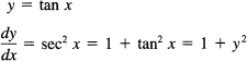
The inverse function has the x and y interchanged:
x = tan y
or, since we need to stick with single-valued functions,
y = Arctan x
Hence we have the general formula
![]()
Note that (like the logarithm) the derivative of the Arctangent is an algebraic function.
Next consider the direct function
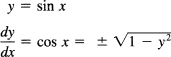
The inverse function is
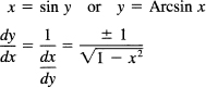
and for the principal value of the Arcsin we need the plus sign. Hence we have the general formula
![]()
Again the derivative is an algebraic function.
The Arccos x goes similarly, except that we must pick the minus sign for the slope of the principal value; hence
![]()
The other three inverse functions are of less importance but are given for the sake of completeness.

The corresponding integrals are
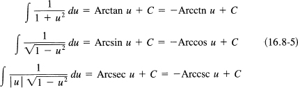
It is important to notice that the inverse trigonometric functions arise from the integration of algebraic functions, as does the logarithm (which is the inverse of the exponential function). As the calculus of the algebraic functions was gradually developed, these inverse trigonometric functions were bound to arise.
Example 16.8-1
Show that
![]()
Integration leads immediately to
![]()
Note that the integral of a simple algebraic function leads to the transcendental number π, which arose originally in connection with the circumference (or area) of a circle.
Example 16.8-2
Integrate
![]()
If we set x = at, we get dx = a dt, and the integral becomes
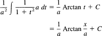
Example 16.8-3
Show that for 0 < x < 1
![]()
We can prove this in many ways. One useful approach is to observe that (from the mean value theorem) if (1) two differentiable functions have the same derivative, and (2) have one point in common, then they are the same function. Hence we differentiate both sides:
For x = 0, we have
Arcsin 0 = 0 = Arccos 1
and we have completed the proof.
Find the following:
1. ![]() Arctan x dx
Arctan x dx
2. ∫ Arcsin x dx
3. ∫ Arctan x dx
4. Show that ![]() [(Arctan x) / 1 + x2) dx] = π /8
[(Arctan x) / 1 + x2) dx] = π /8
5. Show by differenatiation that Arctan x = Arctn 1/ x.
16.9 PROBABILITY PROBLEMS
We are now in a position to examine a number of interesting points that arise in doing probability problems.
Example 16.9-1
A particle is moving in a sinusoidal motion. What is the probability density distribution for finding the particle in the range − 1 to 1? It is no restriction if we assume that the motion is given by
y = sin t
We see immediately that a random sample from the range − π/2 ≤ t ≤ π/2 will be a typical range in which to sample and will give the correct answer. We are selecting a random time (uniformly) in the interval, so we have the probability of falling in the interval dt of
![]()
But
t = Arcsin y
and therefore
From this we get
![]()
The probability density distribution in y is given by
![]()
If this seems strange then you have only to look at Figure 16.1-12 to see that most of the time the particle is near the ends of the range and that it rushes through the middle of the interval. If you are shooting at this target, then aiming at the middle (mean) position is poor policy.
Case Study 16.9-2
A paradox. Lewis Carroll (1832–1898), author of Alice in Wonderland and other children’s stories, was an English mathematician whose real name was Charles Dodgson. He proposed the following problem. Pick three points at random in the plane and form a triangle. What is the probability that the triangle will be obtuse?
His solution was as follows. We pick the coordinate system with the x-axis along the longest side of the triangle with the origin at the end having the shortest side and the length of the unit chosen as the longest side. Figure 16.9-1 shows the sample space and the region of obtuse triangles. It is a matter of computing the two areas and then taking their ratio. For the whole region we have
![]()
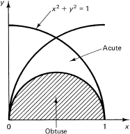
Figure 16.9-1 Base as longest side
Set x = sin θ then dx = cos θ dθ, and the area is
![]()
The region of obtuse triangles is a semicircle of radius 1/2, so the region of successes has an area of π/8. The ratio is
![]()
Suppose we doubt this solution, and chose the coordinate system along the second longest side, with the origin at the vertex with the shortest side. Figure 16.9-2 shows the situation. The other vertex must lie inside the unit circle about the origin and outside the unit circle drawn about the point x = 1. Only to the left of the vertical line through the origin are the triangles obtuse. With slight trouble, we get π/4 for the area of the quadrant. For the area of the small sector, we have
![]()
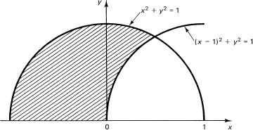
Figure 16.9-2 Second longest side
In the first integral we use x = sin θ, and in the second we use 1 – x = sin θ. We get
![]()
In each we use the half-angle substitution to get
![]()
which gives, finally,
![]()
What is wrong? The first objection that might be raised is the choice of the different coordinate systems. But when you think about it, we assumed that area was independent of coordinate translation and rotation, and you believe that you could find the areas using any coordinate system, although it might be a lot more trouble to do it in some peculiar coordinate systems than in others. We believe that areas are independent of the translation and rotation of the coordinate system, and the scaling does not matter since we are taking ratios of the areas. No, the error is not in the coordinate system rotation and translation.
Maybe the calculus is wrong. But an inspection of the figures shows that the ratios of the computed areas are about correct, and the difference is too large to be explained that way.
We are reduced to thinking hard. As usual, let us go back to a simple problem with the infinite in it. Suppose I ask you to pick a random positive integer. What is its expected value? It is infinite! I mean by those words that you can name any fixed number n you want, no matter how large, and agree that the words “almost all” will be any fraction less than 1 that you care to name; then almost all positive integers are larger than the number n you named. The same sort of argument will apply to choosing any point along a line.
Next we ask, What is the distance between any two random points on an infinite line? The answer is “infinite,” if we similarly understand the word to mean larger than any preassigned number. So when we scaled the units by the length of the longest side, or the second longest side, what were we doing?
The assignment of a uniform probability distribution to the infinite plane is dubious to say the least. Suppose we try to approach the infinite by the usual finite case first. We take a square and imagine that we have solved the problem with a uniform probability assignment and have found the probability of an obtuse triangle. Then we let the side of the square go to infinity. The probability will not change. Next we take an inscribed circle (which cuts off the comers of the square), again with a uniform probability assignment. The probability of an obtuse triangle in the circle will not be the same! We will get a different value for the infinite plane when we let the radius go to infinity. As a more extreme case, consider taking a long, low rectangle, which favors obtuse triangles. Then let the rectangle go to infinity while keeping its shape. Still a different answer.
We begin to realize that no matter how seductive the words may sound, or how many famous people may have fallen into the trap before us, the fact is that we often do not know when a sentence is meaningful and when it is not. The random triangle in the plane seemed reasonable when we started, and apparently seemed reasonable to generations of mathematicians, but now we do not believe that the words say anything definite. Too much more must be said before we think that the problem is well defined. We have a rising standard of rigor, and we probably have not reached the ultimate of rigor; so we need always to keep in mind that maybe we are talking nonsense no matter how fancy the mathematics we use may be.
Example 16.9-3
The Cauchy distribution, or improper integrals revisited. The Cauchy probability distribution density is given by
![]()
The total probability is
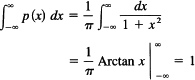
Nothing was said about how we went from the finite limit to the infinite limit; the upper and lower limits were done separately (in our heads).
For probability distributions, the convergence of the absolute value of the integra] of the random variable is required. For the first moment, this means
![]()
must be finite. For the Cauchy distribution, this gives

and the first moment does not exist no matter whether we let the two limits go to infinity together or separately.
If we ignore the absolute value in the first moment (the expected value) of the Cauchy distribution, then we have
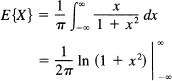
We need to pause and consider matters because the direct substitution would give an infinity at each limit.
If we were to use the limits −a and a and then let a → ∞, we would have
![]()
This is a reasonable answer since the integrand is odd and the interval of integration is even. However, there is a bit of a worry nevertheless, and we look further.
If we let the upper and lower limits of integration approach infinity separately, we would have at the finite stage
![]()
where b is the finite upper limit and −a is the finite lower limit. Now if we suppose that b is proportional to a, say b = ka, then we have, on dividing numerator and denominator by a2,
![]()
and this approaches, as a → ∞,
![]()
We can get any limit we please for the value of the expected value of X.
We face a decision; shall we demand using independent limits for the general improper integral when both ends require attention, or shall we permit the simultaneous, equal approach to the limit? The conventional decision is to demand independent limits, but in some fields of mathematics the simultaneous approach is used and is called the Cauchy principal value. It is foolish to make up the definitions and rules of mathematics without an understanding of the consequences that will follow in your field of interest.
In this case it is known that the Cauchy distribution has peculiar properties. For example, if we wish to estimate the “center” of the distribution
![]()
(estimate a), then the average of n observations is no better than one observation! This result is certainly nonintuitive.
We do not want to commit ourselves universally on what to do in all cases when you have both limits of an integral approaching infinity, one plus and one minus infinity; nor do we want to say that always the absolute value of the randomvariable must converge, since it is conceivable that in some circumstance you might have an ordering of the random variable, but it seems highly unlikely! You have been warned again of the dangers of not thinking carefully about meanings behind the rulesand formulas of mathematics. New applications often require new interpretations of old things. To be ready to create the new things, it is necessary that you understand not only the formal results of past mathematics, but also what assumptions were made, why they were made, and how the assumptions were combined; otherwise, you will be trapped in past thinking. Neither the applications nor formal mathematics is the final judge of definitions and assumptions you make; the decision to make is a blend of the two, involving both what you need and what you can do.
16.10 SUMMARY OF THE INTEGRATION FORMULAS
It is worth assembling the useful integration formulas in one place for easy reference. We make small changes in the notation for convenience.
1. ∫ (au + bv − cw) dx = a ∫ u dx + b ∫ v dx − c ∫ w dx
2. ∫ U dV = UV − ∫ V dU
3. ∫ f(x) = ∫ f(g(t)) g′(t) dt
5. ∫ ![]() du = ln |u| + C
du = ln |u| + C
6. ∫ eu du = eu + C
7. ∫ sin u du = −cos u + C
8. ∫ cos u du = sin u + C
9. ∫ tan u du = ln |sec u| + C
10. ∫ ctn u du = ln |sin u| + C
11. ∫ sec u du = ln |sec u + tan u| + C
12. ∫ csc u du = −ln |csc u + ctn u| + C = ln ![]() + C
+ C
13. ∫ sec2 u du = tan u + C
14. ∫ csc2 u du = − ctn u + C
15. ∫ sec u tan u du = sec u + C
16. ∫ csc u ctn u du = − csc u + C
17. ∫ ![]() du =
du = ![]() arctan
arctan ![]() + C
+ C
18. ∫ ![]() du = arcsin
du = arcsin ![]() + C
+ C
19. ∫ ![]() du =
du = ![]() + C
+ C
20. ∫ ![]() du =
du = ![]() + C
+ C
21. ∫ ![]() du = ln |u +
du = ln |u + ![]() | + C
| + C
22. ∫ (a2 − u2)1/2 du = ![]() +
+ ![]() arcsin
arcsin ![]() + C
+ C
23. ∫ (u2 ± a2)1/2 du = ![]() +
+ ![]() ln (u +
ln (u + ![]() ) + C
) + C
The last five integrals have been added to round out the general forms and are easily derived.
Derive the following formulas from Section 16.10.
1. Formula 19
2. Formula 20
3. Formula 21
4. Formula 22
5. Formula 23
Integrate the following:
6. ∫ 5x / ![]() dx
dx
7. ∫ 5x / (5 − 2x2) dx
8. ∫ x cos 3x dx
9. ∫ (x + 3) / (x2 + 4x + 3) dx
10. ∫ 1 / (x2 − 4x + 4) dx
11. ∫ (ex − 2 + e−2x) dx
12. ∫ 1 / (ex + e−x) dx
13. ∫ ln (1 + ![]() ) dx
) dx
14. ∫ x3 / (x2 + 1) dx
15. ∫ x3 / ![]() dx
dx
16. ∫ e2x sin 3x dx
17. ∫ sin 4(y / 2) dy
18. ∫ {(arcsin x) / (1 −x2)}1/2 dx
19. ∫ (1 + tan t)3 dt
20. ∫ (sin θ) / (1–cos θ)3 dθ
21. ∫ e −t cos at dt
22. ∫ sin 2θ sin 3θ dθ
23. ∫ 1 / ![]() dx
dx
24. ∫ x / ![]() dx
dx
25. ∫ x2 / ![]() dx
dx
26. ∫ x ln (1 − x) dx
27. ∫ arcsin ![]() dx
dx
28. ∫ x2 e−x dx
29. ∫ cos t cos 2t dt
30. ∫ x2 / ![]() dx
dx
31. ∫ (![]() − 1/
− 1/ ![]() )2 dx
)2 dx
32. ∫ sin 3x dx
33. ![]() cos 4x dx
cos 4x dx
34. ![]()
35. ![]() xe−x dx
xe−x dx
36. ![]() x3 exp (−x2 / 2) dx
x3 exp (−x2 / 2) dx
37. ![]() dx
dx
38. ![]() (
(![]() +
+ ![]() ) dx
) dx
39. ![]() ln
ln ![]() dx
dx
16.11 SUMMARY
We first reviewed, in a highly condensed form, the elements of trigonometry. We then examined the problem of finding the derivative of y = sin x. This was first based on an important limit (sin θ)/θ as θ → 0, but later we found the derivative directly from the fundamental theorem of the calculus. In both cases it was necessary to use radian measure to get a formula free of extraneous constants.
We then examined the derivatives and integrals of the various trigonometric functions, as well as their inverses. The inverses all came from the integration of albebraic expressions and show the inevitability of the inverse trigonometric functions arising in many problems.
The next chapter will complete, for a beginning course, the class of functions whose derivatives and integrals you need to know. As a result, you will be ready to tackle a large class of applications of mathematics. We will, at last, have disposed of the more formal details of much of advanced mathematics. It is unfortunate, in a way, that such routine material must be learned before you can get to the interesting, useful applications of mathematics, but there seems to be no way around mastering a minimum of technique if you are to use mathematics, whether to create more mathematics or apply it to other fields.