14.1 INTRODUCTION—A NEW FUNCTION
We have developed the calculus in terms of the simple algebraic functions, and this has limited the class of problems you can do. Part III of the text is devoted to extending the range of functions you can handle, and consequently the range of problems you can do. The main ideas and applications will be repeated in terms of the new functions. Thus there is a great deal of repetition of ideas in this part, the spiral reinforcement of what you have just learned. It is often said that you learn each mathematics course when you use it regularly in the next course. We deliberately and regularly use old ideas, at first reminding you where they came from but gradually assuming that you know them.
We also introduce some new mathematical ideas. The first one is how to study a situation for which you have no already prepared solution. For example, in Part II you had the indefinite integral
![]()
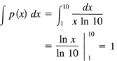
for all n ≠ – 1, but when n = – 1 this formula cannot apply (note the indicated division by 0). This integral
![]()
The integrand does not exist for x = 0, so it is convenient to start the definite integral at x = 1. We will call this the In function (pronounced “the ell en function,” which will soon turn out to be a logarithm function). It is defined by
![]()
It is often convenient to write this as
![]()
when no confusion can arise (it amounts to dropping the constant of integration C).
We know from the existence of the integral (Section 11.5) that since 1/x is continuous for x ≠ 0, the ln x function exists. Are you sure you cannot find some function whose derivative is 1/x? It is evident, after some trial differentiations, that fractional exponents always remain fractional exponents, so you are confined to integer exponents. After some trials, and finding that you cannot find such a function, you are naturally driven to the idea that there is no rational function whose derivative is 1/x, that the ln x is not a rational function in x. In mathematical symbols, this is saying
![]()
where N(x) and D(x) are polynomials of some degrees and the fraction is in lowest terms (meaning no common factors in both the numerator and denominator). You wish to show the nonequality is true, that there can be no two polynomials N(x) and D(x) with the required property. As for most impossibility theorems, the proof is by contradiction.
You may recall from Section 4.6 that polynomials are very much like the integers, and this reminds you that you have seen a similar sort of impossibility problem for the ![]() in the example of Section 3.4. There you had
in the example of Section 3.4. There you had
![]()
as the impossibility; here you have
![]()
What did you do there? You first assumed that there was such an equality, and then squared both sides to get rid of the operation of square root; this suggests that you assume the equality and then differentiate both sides to get rid of the integration. The result is
![]()
Continuing to model this proof on the earlier one, you remove the fractions
![]()
Next was the divisibility argument. Clearly, D(x) is divisible by x; indeed it may be divisible by x several times. Let k be the highest power of x that divides D(x); that is, write
![]()
D0(0) ≠ 0 says that there is no factor x in D0(x). The result is
![]()
Now xk can be divided out to get
![]()
Here each term except the last one is divisible by x, so the last one must be, too. But D0(x) is not divisible by x by its definition; therefore, N(x) must be divisible by x, the same sort of contradiction as before. You assumed that the original expression is in lowest form, and then you found that there is a common factor! Hence the ln x is not a rational function. The proof is a good example of the extension of a method of proof to a similar situation, once you have seen some of the similarities between rational numbers and rational functions.
The function ln x will turn out to be the logarithm of x to the base e = 2.7182818284 … , which is a transcendental number. Hence now is the time for a brief review of the topic of logarithms.
If y is the logarithm of x to the base b, we write this as
![]()
By definition (recall that a logarithm is the power to which the base must be raised to give the original number), it follows that
![]()
Let us take the log to the base a of this equation. We get
![]()
and, since by definition y = logbx, we have
![]()
This says, any system of logs is proportional to any other system. If you have a table of logs to any base (the common logs use base 10), then dividing these entries in the table by the value (from the same table) of the log of the new base, you get the corresponding table in the new base.
If you set x = a in the above equation, you get the useful relationship
![]()
A pair of numbers that are needed in converting from base 10 to base e and back are
![]()
The three relationships you need involving logs are (for any base)
In the last equation, y is any real number. In general, when taking logs, you must start with positive numbers, since the logs of negative numbers are not defined in terms of real numbers. The base is conventionally a positive number greater than 1.
Remember that these are properties of logs, and that we have not yet shown that the integral
![]()
is a logarithm, let alone the actual base involved.
14.2* ln x IS NOT AN ALGEBRAIC FUNCTION
It is slightly less easy to prove that ln x is not an algebraic function. In mathematical terms, this statement means that there is no polynomial in x and y of the form
P(x, y) = 0
such that
![]()
is a solution. The conics of Chapter 6 were algebraic functions where the polynomial was of degree 2. The above assertion is that there can be no polynomial of any finite degree for which y = ln x is a solution. In more detailed mathematical notation this statement is as follows: There can be no polynomial in y with polynomial coefficients in x for which
![]()
for all x in some interval [where the Pk(x) are polynomials in x of arbitrary degrees]. The proof is, as usual, by contradiction. We assume that there is such an equation, and that the degree n is the lowest that is possible in y = ln x. There cannot be more than one polynomial of lowest degree that has the ln x as a solution, since if there were two then we could eliminate the highest power of ln x (by the multiplication of each equation by the coefficient of the highest power of the other followed by a subtraction of the two equations). As a result we would have a still lower degree polynomial (degree in ln x of course), which is not possible since we assumed that we had the lowest.
Using the calculus, we can differentiate this equation. Remember that by the fundamental theorem of the calculus, Section 11.6,
![]()
We obtain another equation
![]()
of the same degree in ln x. Next, by using suitable multipliers and a subtraction, we could eliminate the highest power of ln x to get a lower-degree polynomial and hence a contradiction, provided the resulting equation is not identically zero! We must take care of this possibility. This suggests an alternative approach to the theorem; we should divide through by Pn(x) before the differentiation. You then get, after differentiation,
![]()
The coefficient of the highest power of ln x is
![]()
and is exactly what we just showed (Section 14.1) could not be identically zero. Since the derived polynomial for which ln x is a solution is of lower degree than the one you assumed was of lowest degree, you have a contradiction.
Thus the function ln x is definitely something new, and it is not an algebraic expression in some disguise. We have shown that not only is ln x linearly independent of the powers of x, but that any finite number of integer powers of In Jt are linearly independent, using polynomials in x as coefficients of the powers of ln x. This will be useful later in the book.
1. Carry out the first indicated proof in this section.
2. Prove that In x ≠ N(x)/D(x) using an argument based on the degrees of N(x) and D(x).
14.3 PROPERTIES OF THE FUNCTION ln x
We will investigate this new function using the techniques that have been developed in a field called functional analysis. First, you got rid of the arbitrary constant of the indefinite integral by taking the definite integral form with a fixed lower limit. You did not pick 0 as the lower limit, since at x = 0 the integrand 1/x does not exist. The next natural choice is at x = 1. You have, therefore, the definition (again)
![]()
where it is convenient to use the dummy variable t to avoid confusion with the upper limit of x. Suppose you replace t by a new variable
![]()
for any real n ≠ 0, 1. The integral becomes
![]()
Hence we have the functional equation
![]()
(Normal equations define sets of numbers; functional equations define whole functions.)
Inspection of the functional equation shows that it has the solution
![]()
for any k ≠ 0.
Are there any other solutions to this functional equation? Suppose that g (x) is any solution; hence
![]()
and consider the difference
![]()
For any x0 ≠ 1, set
![]()
Then at x = x0 the left-hand side is zero; hence
![]()
For any real z > 0, there is an n such that
![]()
namely,
![]()
Thus for all real z > 0 we have shown that
![]()
and the solution is essentially unique (within a constant k). The constant k determines the base of the system of logarithms.
The next step is, therefore, to determine the base. What is it that you know? The main property of logs that you know which involves the base b is
![]()
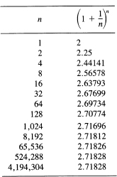
If you integrate numerically, using Simpson’s formula (Section 11.11) from 1 to 3 by double steps of ![]() , you can get an estimate of where the area under the curve 1/x from 1 to x has the value 1. At this point, x will equal the logarithm base. Table 14.3-1 (see also Figure 14.3-1) shows that the base, commonly called e, is approximately
, you can get an estimate of where the area under the curve 1/x from 1 to x has the value 1. At this point, x will equal the logarithm base. Table 14.3-1 (see also Figure 14.3-1) shows that the base, commonly called e, is approximately
e = 2.718
TABLE 14.3-1 ![]()
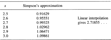
A much more accurate value is
e = 2.71828 18284 59045 …
We will later investigate this number e more closely. It is conventional in mathematics to write logs to the base e as ln x. Logs to the base e are called natural logarithms. They are also called Naperian logs after John Napier (1550–1617), who discovered logarithms, although his were not to the base e in spite of what you may read in some books. We have already used the notation logbx for other bases, with log x meaning base 10.
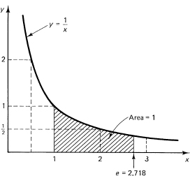
Figure 14.3-1 Estimate of e
Write the value of the following in terms of In 2 and In 3:
1. ln 9
2. ln 12
3. ln (33)
4. ln ![]()
5. (ln ![]() )2
)2
6. ln 24
7. 3 ln ![]()
8. ln (3/2)3
9. 4 ln 1/4
10. ![]()
What are the following?
11. ln2 4
12. ln4 8
13. (ln ![]() )2
)2
14. ln10 100
14.4 AN ALTERNATIVE DERIVATION—COMPOUND INTEREST
Since we have regularly preached going back to basics, how would the direct derivation of the derivative of ln x go? We apply the four-step rule (Section 7.5) to the loga x function. At the third step we have
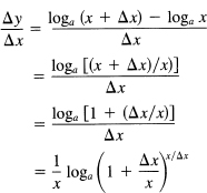
We need to examine the limit of
![]()
as ![]() x → 0. Set x/
x → 0. Set x/![]() x = t. The limit is now the same as
x = t. The limit is now the same as
![]()
as t → ∞. We could instead set t = 1/u and have the limit
![]()
as u → 0. The three limits are clearly equivalent. From the following table of numbers, it seems as if the limit is the same number e = 2.71828 … as before.
![]()
For a = e, this becomes
![]()
The three limits occur frequently.
Example 14.4-1
Compound interest. This limit e occurs in compound interest problems. Suppose you have an interest rate r of 6%, 12%, or 18% as given in the headings of the columns of Table 14.4-2. The left-hand column has the number of compounding periods. The first line gives the growth per year on 1 unit of money (or other quantity such as biological size). The entry in the body of the table is simply the total amount, interest plus original amount for one period. The second line is for compounding each quarter, the rate per quarter is one-quarter as much, but you get the interest four times plus the interest on the interest. The formula is, for rate r,
![]()
The first two terms account for the principal and the original simple interest, and the later terms are the interest on the interest due to the compounding.
Next, suppose it is compounded monthly. The effective rate is r/12 per month, and it is compounded 12 times. Finally, consider compounding daily. The daily rate is r/365, and it is done 365 times.
TABLE 14.4-2
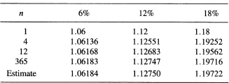
We see that the numbers approach limits, and we see that well before we are at 365 we are close to the position where we could use the number e. We have, corresponding to (14.4-2), the limit
![]()
Using this, estimates are written at the bottom of the columns of the table. These values correspond to continuous compounding.
This is another example of the fact that, although the phenomenon you are studying may be discrete (a finite number of fixed sized events), nevertheless the continuous model of the calculus provides a very convenient tool for getting good approximations.
1. Show that ![]() 1/x dx = 2 ln 10.
1/x dx = 2 ln 10.
2. Show that, for any function f(x) and ![]() Hint: Use the reciprocal substitution.
Hint: Use the reciprocal substitution.
3. Compute the estimate in Table 14.4-2 for 8% interest.
4. Find a formula for the doubling period at any given rate of compounding.
5. Make a table of the doubling periods and compare with the following classic rule: Divide 72 by the rate (expressed as a percent) to get the number of years to double.
14.5 FORMAL DIFFERENTIATION AND INTEGRATION INVOLVING ln x
We need to look at the differentiation and integration of this new function. As the first few examples show, there are often ways of simplifying the expression before differentiation.
Example 14.5-1
Compute
Find dy/dx where
![]()
Take the In of both sides before differentiating (and use the function of a function idea):
![]()
We see that each term is to be differentiated separately, and this makes things much easier.
![]()
It is important to note that if x is replaced by –x in the integral, then the dx is replaced by – dx, and the quantity
![]()
does not change! Thus in truth
![]()
We simply cannot tell which sign to use when we are given the derivative. Usually, the problem indicates which sign to use, but as protection we must remember that all we get is the absolute size, not the algebraic size.
Example 14.5-2
Differentiate
y = ln(1 + x2)
We get immediately (U = 1 + x2; note that we have shifted from the lower case u to the upper case U)
Example 14.5-3
Differentiate
![]()
This gives
![]()
Example 14.5-4
Differentiate
![]()
This gives
![]()
Integrate
![]()
If we think of the denominator as U = 1 + x, then the dU = dx, and we have (1/U) dU to integrate. The result is
![]()
Example 14.5-6
Integrate
![]()
This time we pick U = 1 + x2 and need dU = 2x dx. We lack a factor 2, so we supply it inside the integral and compensate by a factor of ![]() in front. Thus
in front. Thus
![]()
Differentiation will verify it easily.
![]()
Example 14.5-7
Integrate
![]()
Here we appear to be in trouble since there is no x in the numerator for the derivative of the denominator. After some thought, we notice that a2 – x2 = (a – x)(a + x), and that maybe the term came from the sum of two terms of the form
![]()
We do not know the actual numerators, so we apply the method of undetermined coefficients and write
![]()
with A and B the undetermined coefficients. Cleared of fractions,
![]()
From the linear independence of the powers of x, we may equate like powers of x. We get form the x terms
A = B
Then from the constant terms we get
2aA = 1
Hence
![]()
It is easy to check this result by adding the two terms together. The integral is, therefore,
This can be verified by differentiating.
Example 14.5-8
Integrate
![]()
Set U = ln x, and we have the form U dU, which leads to U2/2:
![]()
Example 14.5-9
Integrate
![]()
The ln x in the denominator looks difficult to handle. How could it have gotten there from a differentiation? Well, a log does that, so we finally think of
ln |ln x| + C
as the answer. Differentiation checks our guess.
Example 14.5-10.
Integrate
![]()
This lacks a 3 in the numerator of being just right, dU/U. Thus the integral must be
![]()
which is easily verified by differentiation.
Differentiate the following on sight:
1. y = ![]()
2. y = x2 ln x
3. y = ln (x3 – 3x)
4. y = xn x xn/n
Integrate the following:
5. ∫ 1/(1 + x) dx
6. ∫ 1/(a + bx) dx
7. ∫ 1/(a + bx)2 dx
8. ∫ x/(1 + x2) dx
9. ∫ x/(a2 + x2) dx
10. ∫ x/(a2 + x2)2 dx
11. ∫ (ln x)2/x dx = |ln x|3/3 + C
12. ∫ (ln3 x)/x dx
13. ∫ (lna x)/x dx
14. ![]()
15. ∫ (1/x)(1 + ln x)dx
16. ∫ 1/{x (1 + ln x)}dx
14.6 APPLICATIONS
The curve y = ln x rises smoothly but increasingly slowly as you go from x = 1 (y = 0) to the right (Figure 14.6-1). Each time you go a distance e = 2.71828 … times as far out, you rise by another unit; the curve becomes very flat, but continues to rise indefinitely (since y′ = 1/x > 0 for x > 0). There is no upper bound of the ln x function. The second derivative is –1/x2 and is always negative, so the curve is always concave downward. Since ln 1/x = –ln x, the values going to the left of x = 1 head toward minus infinity as x → 0.
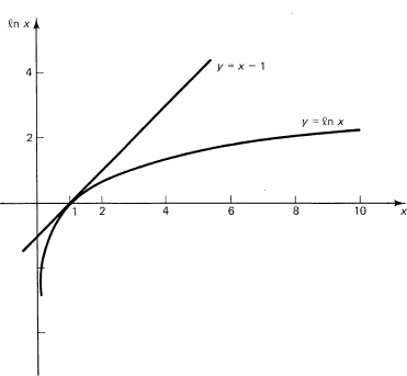
Figure 14.6-1 The ln x function
Example 14.6-1
Graph the function
![]()
(which occurs frequently). To study it near the origin where one factor is 0 and the other is arbitrarily large, we compute Table 14.6-1.
TABLE 14.6.1
| x | x ln x |
| 0.1 | −0.23026 |
| 0.01 | −0.04605 |
| 0.001 | −0.00691 |
| 0.0001 | −0.00092 |
We see why we think that the limit is zero. We will later prove in a more mathematical setting (Section 15.5) that the limit is zero. At the origin, the zero from the term x dominates the infinity from the term ln x. Thus the function
y = x ln x
has a pair of zeros (Figure 14.6-2), one at x = 0 and the other at x = 1, and between them the function is negative. Where does the minimum occur? Differentiate, set equal to zero, and solve.
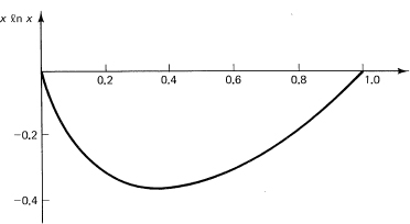
Figure 14.6-2 y = x ln x
![]()
or
ln x = –1
Hence the minimum occurs at x = 1/e. At this point
![]()
Since y″ = 1/x > 0, this indicates that the curve is always (for x > 0) convex upward.
Example 14.6-2
The entropy function, which is defined for any discrete probability distribution pi is given by the expression
![]()
where ∑ pi = 1 and P represents the probability distribution, or if you wish the random variable. This function occurs in many places, particularly in information and coding theory; and as is customary there, we have taken 2 as the base of the logarithm system (also to give you practice in other bases than e and 10). In words, the entropy of a distribution is the probability-weighted average of the negative logarithms of the probabilities of the distribution.
It is natural to ask for the set of probabilities pt for which the entropy function Hn(P) is maximum. By a study of the way each individual term of the function behaves (see Figure 14.6-2), and recognizing that since ∑ pi = 1, then any increase in one term must decrease some other term, you soon come to the conclusion that the symmetric case must give the maximum, all the
![]()
Alternatively, you can eliminate one of the probabilities, say pn, by using the relation
![]()
![]()
and when you differentiate with respect to pi (for each i = 1, … , n – 1), you get for each derivative equated to zero [recall (14.4-4) and write 1 – p1 – p2 – … – pn–1 = pn after the differentiation]
![]()
Thus
![]()
and each pi = pn (because the log function is monotone and therefore there is only one solution for a given value of the function). Hence, since the sum of all the pi is 1, it follows that each pi = 1/n. What is the maximum value? Putpi = 1/n in each term and you get n terms, each of which is
![]()
so the sum of all n terms gives the maximum
![]()
Example 14.6-3
The Gibbs inequality (used extensively in information theory and probability). Given two discrete probability distributions
![]()
show that
![]()
To prove this we need a simple lemma.
Lemma. For all x >0
![]()
and the equality holds only at x = 1.
The proof is easy; we simply fit the tangent line to the curve y = ln x at the point x = 1 (Figure 14.6-1) and note that the curve is below the tangent line. The derivative of ln x is 1/x, and at x = 1 this is 1. The tangent line, therefore, is
y – 0 = 1(x − 1)
The second derivative of ln x is –1/x2, which is always negative, and this leads to the statement of the lemma (14.6-6).
To prove the main result, we simply apply this lemma to each term of the sum (14.6-5):
![]()
For the equality condition to hold, it must hold for each term of the sum; that is, each qi = pi for all i. This is known as the Gibbs (1839–1903) inequality. The inequality applies for any base b > 1.
EXERCISES 14.6
1. Sketch H2(P) = p log2 (1/p) + (1 – p) log2 1/(1 – p) when the distribution has only two probabilities, p and 1 – p. Note carefully the slope at p = 0 and p = 1.
2. From the Gibbs inequality, show directly that a maximum of the entropy function is ln n. Hint: Set qi = 1/n for all i.
3. Prove from Exercise 2 that the maximum entropy occurs when all the pi are equal.
14.7 INTEGRATION BY PARTS
One of the most useful tools for integration is the method of integration by parts. It is easily derived from the formula for the product of two functions (in differential form)
d(uv) = u dv + v du
We merely take the indefinite integral of both sides (and neglect the constant C of integration). We get
![]()
or in the standard form (where we shift to the conventional uppercase letters)
![]()
The lost constant of integration can be associated with the second integral if you are worried about it.
The reason that the method is so important is that when you see an awkward function under the integral sign then calling it U means that you will later see it only as the derivative (which is often simpler than the function!). We will illustrate this observation by a series of examples.
Example 14.7-1.
Consider the integral
![]()
At first you are probably stunned by the appearance of the In x. You probably do not know an integral of it. But the above remark suggests that you can get rid of the ln x if you pick U = ln x and the rest as the dV. You have
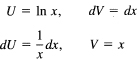
(It is usually convenient to pick the constant of integrating C when integration dV as 0, as we have done, but occasionally other choices are useful.) Using the formula for integration by parts (14.7-1), you have for the given integral
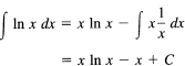
You can verify this easily by differentiating the answer. You get
![]()
which is indeed the integrand.
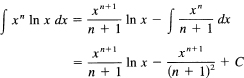
Example 14.7-2
Next consider the integral
![]()
How would you proceed? Pick U as x ln x? That would still leave a ln x after the differentiation to get the dU. This could be done by another application of integration by parts, but perhaps
would be better. So you try it. You get
![]()
and the second integral can now be done. You get, finally,
![]()
which you then verify by differentiating back to check that the integrand comes out.
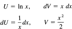
Generalization 14.7-3
Generalize the previous two examples. One possible generalization is
![]()
To get rid of the unwanted ln x function, you pick it as
U = ln x
That leaves the rest as the dV:
![]()
You have
![]()
and therefore
Again you verify by direct differentiation. With this simple check there is no excuse for giving a wrong answer; the only possible excuse is that you could not get started on the problem correctly! Note that this generalization provides a check on the two previous examples, n = 0 and n = 1. The formula is true for all real n ≠ – 1.
Example 14.7-4
Consider
![]()
Obviously, you pick U = (ln x)2 = ln2 x, and dV = dx. You get
![]()
The x terms cancel in the second integrand, and you have
![]()
You are now reduced to an earlier case, Example 14.7-1, which will yield to another integration by parts. Thus you have, finally,
![]()
To check the answer, you differentiate the result. You get from differentiating the right-hand side
![]()
and all the terms cancel, as they should, except the first one. This kind of cancellation is very typical of results obtained by repeated integration by parts.
Example 14.7-5
An example that usually bothers the student the first time it occurs is
![]()
This is the missing case n = –1 in Generalization 14.7-3. There are many ways of doing it. There is the direct way used in Section 14.5 (not integration by parts)
![]()
which gives, as before,
![]()
If you try integration by parts, you get
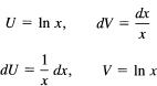
Notice the advantage of the fixed pattern for writing the terms you are going to use. The use of the same technique every time frees the mind for more important things. When you do the integration by parts, you get
![]()
The integral on the right end is the same as the original integral! A moment’s thought shows that you can transpose it to the left-hand side, divide through by 2 (and remember to attach the constant C) to get
![]()
as you should.
There are often several ways of doing the same integral. We have apparently neglected to handle the absolute values in doing the integration; this leaves you a problem to discuss for your own peace of mind. The results must, of course, be the same within an additive constant C. Note that ln 6x + C and ln x + C are the same (although the two values of the constant C differ by the number ln 6).
Integrate the following:
1. ∫ x3 ln x dx
2. ∫ P(x) ln x dx, where P(x) is an arbitrary polynomial. Hint: write P(x) = ΣN0 ckxk.
3. ∫ lnn x dx
4. Carry out one stage of the general case J(m,n) = ∫ xm lnn x dx to get a reduction formula lowering the degree of n to n – 1. J(m, n) = xm+1(lnn x)/(m + 1) – n/(m + 1)J(m, n – 1).
5. Discuss why any polynomial in x and ln x can be integrated in principle.
6. In the above exercises, when can the implied condition of integer exponents be relaxed?
7. Why do we not use the derivative of a quotient formula as the basis for two corresponding integration formulas?
14.8* THE DISTRIBUTION OF NUMBERS
The widely used scientific notation for representing numbers places the decimal point after the first nonzero digit and follows the number by an appropriate power of 10; for example
![]()
The velocity of light is approximately 299,792.5 kilometers per second, and is written as
c = 2.997 925 × 105
Likewise 1/1000 is written as
1 × 10⁻³
The number part is often carelessly called the mantissa in analogy with the mantissa of logarithms.
You might think that these mantissas are uniformly distributed between 1 and 10, but simple experiments do not bear this out. Rather, for most (but not all) sources of numbers the probability density is close to
![]()
where b is the number base, in the usual case 10, but in computers it may be 2, 8, or 16. This distribution is often called the reciprocal distribution because p (x) is proportional to the reciprocal of x. The cumulative probability distribution for the random variable X is (1 ≤ x < b), P(X ≤ x) = P(x)
![]()
In computers it is usual to place the decimal point before the first digit, thus making the exponent 1 greater. The difference is a trivial nuisance, but it is probably too late to get the computer people to reform. In any case, the density distribution is essentially the same, (ln fax)/ln fa. We will use the conventional scientific notation and the interval (sample space) 1 ≤ x < 10.
It is easy to verify that the total probability, using base 10, is
The cumulative distribution for the random variable X is P(x) = ln x/ln 10 = logio x. What is the probability of a random number beginning with a given decimal digit? For the digit N, it is the difference
![]()
As an experimental test of the distribution, we took the 50 physical constants listed in a standard table and counted the number of entries beginning with each decimal digit. The result is given in Table 14.8-1,
TABLE 14.8-1
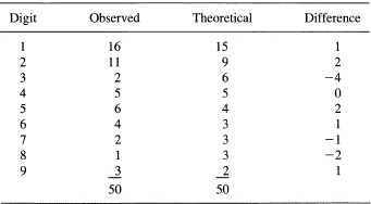
which seems to verify the model for physical constants. The distribution also applies to such widely diverse sources of numbers as the binomial coefficients, the factorials, the powers of any number whose logio is not a rational number, and so on.
The nonuniform distribution of the numbers has a number of consequences. For example, the effect of roundoff propagating through a sequence of multiplications depends, on the average, on the distribution of the leading digits, since if we have two numbers with corresponding small errors
![]()
and form their product, we get
x1x2 + x1![]() 2 + x1
2 + x1![]() 1 +
1 + ![]() 1
1![]() 2
2
Neglecting the last term as being too small to matter, we see that the expected value of the xi gives the effective multiplier of each propagated error for randomly chosen numbers.
Example 14.8-1
Find the expected value of a number from the reciprocal distribution. We have
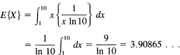
which is a good deal less than the 5.5 that is given by the model of a uniform distribution.
1. Make a table of the distribution of the first digit of the function 2n for n = 1, … ,25.
2. Same for y = 3n.
3. Same for y = 5n.
4. Compute the distributionof leading digits forthe base 8.
5. Compute the expected propagationcoefficient for base b and examine the results for the bases 2, 4, 8, 10, and 16.
6. Find the variance of the reciprocal distribution.
14.9 IMPROPER INTEGRALS
Up to this point we have insisted that the integral have two properties. First, that the range of integration, typically from a to b, be finite. Second, that in the range of integration the integrand be finite. Without these two conditions the derivations we made in connection with the development of the concept of the integral would not be valid.
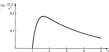
Figure 14.9-1 ![]()
However, frequently problems arise where one or the other (or both) of these conditions is violated. As an example of an infinite range, consider the area under the curve
![]()
from x = 1 to x = ∞ (see Figure 14.9-1). An example of an infinite integrand is the area below the curve
y = –ln x
above the x-axis and between x = 0 and x = 1 (see Figure 14.9-2). We treat both cases by the following very reasonable device. We ask, “What is the integral when the range is chosen to be slightly less?” and then we examine the answer as the range is increased to the limit, either (1) for infinite range or (2) to where the integrand becomes infinite.
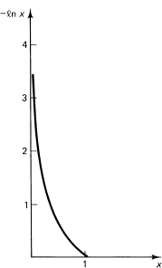
Figure 14.9-2 y = —ln x
This process of handling the infinite by dropping back to the finite, working out the result, and then taking the limit is a basic approach, which we have already used many times. When in doubt, it is a sound rule: “Do the finite case, and then examine how it behaves as you approach infinity.” If the result appears strange, then you are in a position to see whether it is your intuition or an error that bothers you.
Example 14.9-1
We first consider the case of an infinite range. In this example we begin by considering the integral over the finite range
![]()
(Figure 14.9-1). When we get the answer in terms of N, we will then let N approach infinity. To do the integration, we use integration by parts with
The indefinite integral becomes
We have now to put in the limits 1 and N. We get the definite integral
![]()
We are now ready to let N approach infinity. The first term, – (In N)/N, requires attention. As before, the denominator N dominates the slower growing numerator In N, and the quotient goes to 0. The final answer is, therefore,
J(∞) = 1
The area under the curve y = (In x)/x2 from x = 1 to infinity is exactly 1.
Example 14.9-2
An example of the infinite integrand is the area between
y = –ln x
the x-axis, and in the interval x = 0 to x = 1 (see Figure 14.9-2). We have to creep down to the origin, so we start with the integral (with a > 0):
We now let a approach 0. Again the a dominates the In a as a approaches 0. The final result is
J(0) = 1
There is one unit of area below the -In x curve and above the x-axis while lying between x = 0 and x = 1.
Example 14.9-3
Suppose the curve y = –ln x for (0 < x ≤ 1) is rotated about the y-axis to form a volume of rotation (see Figure 14.9-3). What is the volume? Again, there is an improper integral to evaluate. From the figure, the elements (of volume) we are summing are cylinders, each of volume
2πxy dx
Thus we have (and we eliminate, except in our minds, all the details of letting the lower value approach 0)
![]()
We get
![]()
for the volume of rotation. The direct substitution of the value 0 masks the careful process of examining the value obtained. This can at times lead to troubles, for example, when terms from two different places both cancel before putting in the limit. You should be prepared to follow the longer path of carefully filling in all the details in any doubtful situation.
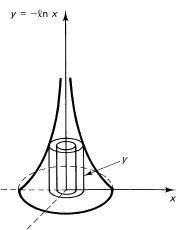
Figure 14.9-3 Method of cylinders
The same problem can be done using discs instead of cylinders (Figure 14.9-4). We have the element of volume
πx2 dy
so we have the integral
![]()
We will change the variable of integration from dy to dx using the equation
![]()
The limits, of course, also change. The infinity for y becomes x = 0, and y = 0 becomes x = 1. We have, therefore (remember the minus sign),
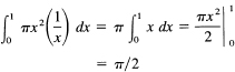
as before.
Figure 14.9-4 Method of discs
Example 14.9-5
Sometimes (as in Example 14.9-4) a change of variable will eliminate an improper integral. Another example is, given the integral
![]()
the change of variable x = 1/y, dx = –1/y2 dy will give
Evaluate the following:
1. ![]()
2. ![]()
3. ![]()
4. Find the area under H(P) = p ln 1/p + (1 – p) between 0 and 1.
5. Integrate ![]()
6. Eliminate the improper integral ![]() by the substitution x = 1/y.
by the substitution x = 1/y.
14.10 SYSTEMATIC INTEGRATION
As you approach the problem of integration, it usually appears as a vast morass of special cases, some of which can be done by one trick, some by another, and some which cannot be done within the framework of a given set of functions. For example, the integral
![]()
cannot be done in closed form (a finite combination of elementary functions). On the other hand, the integral
![]()
But we have preached the necessity of the larger view, the uniformization of special tricks, the need for abstraction to master the sea of details, and the corresponding hopelessness of going down the path of special tricks for the endless number of special cases. It is necessary, therefore, to look a bit more abstractly at the problem of integration of functions involving the function ln x. In particular, what broad classes of integrals can be integrated in closed form? There will still be special isolated cases that require tricks to integrate, but at least we will know some of the general cases we can hope to handle.
From the Generalization 14.7-3 that
![]()
![]()
where P(x) is any polynomial of degree n in x, can be integrated. We see that the form of the result is
![]()
If we apply the fundamental theorem of the calculus to this, we have (differentiate)
![]()
But we proved (Section 14.1) the important result that the ln x cannot be represented by a rational function (indeed we proved in Section 14.2* that the powers of ln x are linearly independent when the coefficients are polynomials). Therefore, we may equate all the terms in ln x to zero and the terms free of ln x to zero. We get
![]()
from which we get
We picked the lower limit in the first integral to be zero so that in the next integrand Q(x)/x is a polynomial.
Example 14.10-1
Integrate
![]()
We try the form
![]()
Upon differentiating both expressions, we get
![]()
Equating the coefficients, one by one, of the two In terms, we get
![]()
Now equating the terms without the ln function, we get, in sequence,
![]()
The integral is, therefore,
![]()
Upon differentiation, this easily checks.
This method of integration is a general one, but it is usually neglected in the standard textbooks. It is a powerful method worth remembering. First, you guess at the form (as you often do in the method of undetermined coefficients). Second, you apply the fundamental theorem of the calculus (differentiate both sides). Third, you equate the coefficients of the linearly independent functions to zero, thus getting as many conditions as there are unknowns in the form you assumed. As in the method of undetermined coefficients, if you guess the form wrong, you will find out that you are wrong and often get a clue as to where you were wrong. You can then either include more terms as suggested by the failure, or else set about proving that it cannot be done in the general form you are trying (see Sections 14.1 and 14.2*).
The approach depends on your understanding of what terms can possibly lead to the integrand you are given and what terms simply cannot be involved. Thus it should be clear that radicals when differentiated lead to radicals and, therefore, cannot be involved in a problem where the integrand is rational. You can fill in the details of the argument to convince yourself that if you try such a term it will end up with a zero coefficient (when you equate such linearly independent terms to zero).
Evidently, the method that assumes the form is often easier to carry out than the equivalent method of direct integration (using repeated integration by parts in this case).
The method is easily extended to
![]()
and then you see that the entire class
![]()
can be done, where now P(x, ln x) is the polynomial in two variables x and In x.
Why can these integrals be done? One partial explanation is that the ln x function arises from the integration of a rational function 1/x, and therefore when we either integrate by parts or differentiate in the above method, the In function effectively disappears.
1. Write out the form you would assume for the integration of P(x, ln x).
2. Carry out the details for the integrand P(x) ln2x.
3.* Following the pattern of Section 14.2*, show that ∫ 1/ln x dx ≠ N (x, ln x)/D (x, ln x), where N(x, ln x) and D(x, ln x) are polynomials.
14.11 SUMMARY
We introduced and studied a new function ln x. It was defined by an integral, which we proved could not be done in a closed rational (or algebraic) form. We further showed that the powers of ln x were linearly independent, and this is useful in the later stages of the systematic integration of integrals with powers of ln x.
We also examined the use of the new function in a number of old and new applications, including compound interest, the distribution of numbers, and the entropy function.
The powerful method of integration by parts was introduced; it is simply the inverse of the derivative of a product. The method enables you to replace a function by its derivative in the new integral, which is often, when combined with the integral of the other part of the integrand, such that you can carry out an integration. Integration by parts and the method of changing variables are two of the most powerful methods of integration available.
We also extended the idea of an integral to improper integrals by the usual method of examining the finite case and letting it approach infinity. In general, it is not the details but the methods used to develop new applications that are important.
Finally, we introduced the obvious “guess at the solution” method as another illustration of the usefulness of the method of undetermined coefficients. If you guess the correct form, then from the fundamental theorem of calculus you can equate the derivative of your guess to the original integrand. If the result is an identity, for a suitable choice of the undetermined parameters you introduced into the guessed form, then you have the integral. If it is not an identity, then you can guess again, guided by the failure to fit, or else abandon that approach.