18.1 INTRODUCTION
Now that we have a reasonable ability to integrate various functions, we can return to the applications of the ideas of the calculus. This time we do not need to pick the applications carefully, as we did earlier, so that the resulting integrals can be done by very limited tools. It is worth repeating that the calculus was developed, to a great extent, as a method for solving problems that arose in mechanics and related fields; but we will look only briefly at these applications.
We will first review a few of the kinds of applications that we have done, using our greater range of functions, and then turn to new applications. Thus we are partially reinforcing the earlier learning.
Calculus, probability, and statistics may each be studied for their own interest. For example, we looked at how little we had to initially derive (by the A process) in order to find all the derivatives we needed. Similarly, we looked slightly at the bases of both probability and statistics. On the other hand, these three fields may be looked at in terms of the problems they allow us to solve, the applications we can make. Both views are legitimate ones to take. They tend in practice to supplement each other.
18.2 WORD PROBLEMS
When we apply mathematics we form a model of the situation (see Figure 9.3-2). Mathematics cannot be applied directly to the real world; it can only be applied to the model we form of reality. In practice, the model we form rests on intuitive bases, partly arising from experience and partly from fairly direct understanding of the world and the model. The purpose of this chapter is to increase your experience in using the mathematics that you already have learned (and to reinforce this learning).
The application of mathematics implies word problems. These problems are often difficult for the student to handle. Real-life problems are usually much more difficult than are textbook problems. The first, and usually the most difficult, step in real-life problems is to recognize that there is a problem to solve. The next most difficult step is to formulate the problem properly. When these two steps have been taken, you are at the stage of doing word problems.
The usual advice to the student is, “Understand the problem first before you try to solve it.” Unfortunately, these words are of little practical value since the main difficulty is that rereading the problem often produces no further understanding. There is no magic solution to the dilemma, but there are some helpful things you can do.
Read the problem and find out what is being asked. Give it a name, typically x; but if you see that you will need a coordinate system, maybe you should save x for the corresponding coordinate. It is surprising how powerful is the single step of naming things; it gives you a feeling of mastery over the situation, it is the first step in any science. Then reread the problem assigning names to the various items, a, y, c, and so on. Along with the naming process, you make a picture of the situation. Together, the two processes of naming and drawing a picture often produce an increased understanding of the problem, at least enough to allow you to go forward. It is quite common that you have to abandon one or more of the figures and redraw them as your understanding of the problem progresses. Sometimes you will also have to relabel things a bit. With luck, after several iterations of this process, you will have a fairly clear idea of the problem.
However, some problems do not permit drawing useful pictures, as the following classic example shows. In this problem, you merely rewrite the original statements of the problem in equivalent, more useful, forms, a characteristic feature of mathematics.
Example 18.2-1
If a hen and a half lays an egg and a half in a day and a half, how long does it take for 6 hens to lay 8 eggs?
The problem is designed to be confusing! Therefore, we read it carefully, translating the words to more common usage as we go. “If a hen and a half lays an egg and a half …” means the same as “If one hen lays one egg … Now, “If one hen lays one egg in a day and a half …” means “One hen lays 2/3 of an egg per day … .” Hence, 6 hens will lay 6(2/3) = 4 eggs in one day. From this it follows that to lay 8 eggs will take 8/4 = 2 days. The answer is, therefore, two days.
Once the textbook problem is understood and properly formulated, it is a matter of applying the techniques you have just learned, or possibly slightly extending them, to get the answer. Of course, the solution may also depend on things that you learned long ago in this course or earlier courses. But usually in textbooks the mathematical tools required are related to the material just covered.
In real life this sorting out of the problems according to the tools needed for their solution does not occur. Even when you have a clear formulation of a problem you may still not know what mathematical tools will be needed to solve it. Giving you carefully selected word problems is about as close as an elementary textbook can come to real-world situations.
The calculus not only opens the door on the solution of word problems, but you have also arrived at the stage where applications to new kinds of questions can be made easily. Hence many of the new applications in this chapter should be viewed as merely larger-than-usual word problems.
18.3 REVIEW OF APPLICATIONS
The applications of derivatives were to (1) curves, especially curve tracing, (2) maxima and minima problems, (3) rate problems, (4) generating functions, (5) least squares, (6) maximum likelihood, and finally (7) indeterminate forms. The applications of integration included the computation of (1) areas, (2) volumes of rotation, and (3) probability. We do a few examples for purposes of review.
Example 18.3-1
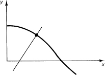
Given the curve
y = cos x
is there a normal line that passes through the origin? See Figure 18.3-1. We know immediately that we need the derivative
y′ = −sinx
Figure 18.3-1 Normal line
At the point (x1, y1 the normal line has the negative reciprocal slope of the tangent line; hence the equation of the normal line is
![]()
If this line is to pass through the origin, then the point (0, 0) must lie on the line
![]()
sin 2x1 = 2x1
The only solution of this equation is x1 = 0. This line, x = 0, is a vertical line through the origin.
Example 18.3-2
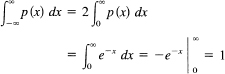
Sketch the normal distribution
![]()
The curve will later be shown (Example 19.4-4) to have an integral equal to 1; thus y(x) can represent a probability distribution. First, since x occurs only in even powers, there is symmetry about the y-axis. Next, we compute y′(x) and y″(x). We get
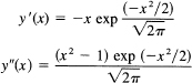
We see that ![]() y′ = 0; and
y′ = 0; and ![]() . The inflection points occur where y″ = 0 and these are x = ± 1. The value of the function
. The inflection points occur where y″ = 0 and these are x = ± 1. The value of the function ![]() . The slope
. The slope ![]() at the inflection points is also useful for plotting the curve. With this tied down, and the knowledge that as x → ∞ the curve rapidly approaches 0, we can draw Figure 18.3-2.
at the inflection points is also useful for plotting the curve. With this tied down, and the knowledge that as x → ∞ the curve rapidly approaches 0, we can draw Figure 18.3-2.
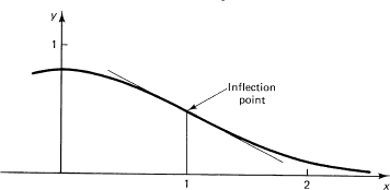
Figure 18.3-2 Error curve
The applications of integrals is much more varied, and we give only a few examples.
Example 18.3-3
Find the maximum area of the ellipse
![]()
when a + b = 1. We must first find the area of the ellipse. We have (from symmetry)
![]()
In this we set x = a sin θ. We get
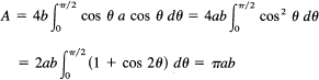
We now know that the area of the ellipse is ∏xsab; hence we have the simple problem of finding the maximum of a product when the sum a + b = 1. We have the area
![]()
from which it follows that a = ½ = b, and we have a circle whose area is A = π/4
Example 18.3-4
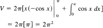
Find the volume of one arch of y = sin x between 0 and π when the curve is rotated about the x-axis. The volume is given by (see Figure 18.3-3), using discs as shown,
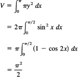
which is less than the enclosing cylinder, π2, by a reasonable amount. A lower bound of an enclosed double cone is easily found to be π2/3.
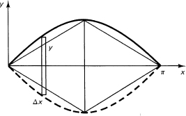
Figure 18.3-3
Example 18.3-5
Find the volume generated by the area under y = sin x, from 0 to π, and above the x-axis, when rotated about the y-axis (see Figure 18.3-4). The volume is, using the element of volume as a cylinder (as shown),
Figure 18.3-4
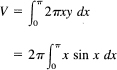
We naturally apply integration by parts to remove the x factor.
The volume of the enclosing cylinder is π3.
Example 18.3-6
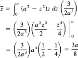
What is the variance of the distribution
![]()
First, we need to check that it is a distribution. We have, due to the symmetry and the obvious convergence of the integral,
Again, by symmetry, the first moment is zero; hence the variance is
![]()
1. Find the tangent line to y = xn at x = 1.
2. Find the tangent line to x2 + y2 − 4x + 3 = 0 through the origin.
3. Find the equations giving the positions of the max-min and inflection points for the curve y = exp (−ax) cos bx.
4. Find the formula giving the shape of the maximum volume for a cylindrical block fitting inside one arch of y = sin x rotated about the x-axis.
5. Given the curve (0, ∞) y = exp (−ax) sin bx (a >0), find the area under the square of the curve.
6. Rotate the curve y = xn exp (−x)/n! about the x-axis. Find the volume from 0 to infinity. (Hint: Remember the gamma function.) Use Stirling’s formula to approximate the answer for large n.
7. Sketch y = exp (−x4 / 4).
8. Given y = ln x(0 < x ≤ l) rotated about the y-axis. Find the rate at which the surface falls when x = 1 / 2 and the rate of decrease in the volume is 4 units per second.
9. Approximate y = sin x (0, π / 2) by a straight line in a least squares sense.
10. Show that ![]()
18.4 ARC LENGTH
We now turn to new applications that use the same ideas as we developed earlier. These applications are slightly more difficult to do than the above word problems. However, you need practice in applying what you have learned to situations that have not been previously explained in detail to you.
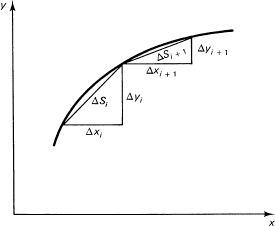
A topic that will arise, sooner or later, is that of the length of a curve. Just as we extended the idea of area from triangles and rectangles to curved regions, so too we now extend our ideas of the length of a straight line segment to curved lines. The basic definition of length is that of a line segment. The extension to a circle in geometry comes from taking the limit of secant lines through points on the circle as the largest interval approaches zero length. This is analogous to what was done for areas. Intuitively, the length of the circumference of a circle comes from the feeling of rolling the circle along a plane surface and measuring how far the rim goes while completing a full revolution of the circle. For curves other than convex ones, we cannot do this. We can, of course, imagine a string that is glued to the edge and later unwound. This is very much like using short secant lines. As with areas, we propose to use a general approach, and not one tied to a particular curve.
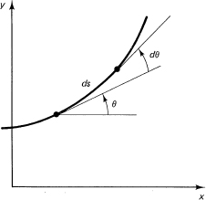
Consider a curve (Figure 18.4-1) with the short secant lines drawn in. We see many small triangles each with the property that the horizontal distance is ![]() xi, the vertical distance is
xi, the vertical distance is ![]() yi and the hypotenuse is
yi and the hypotenuse is ![]() si. This is the elementary triangle. We have, dropping the subscripts,
si. This is the elementary triangle. We have, dropping the subscripts,
![]()
If we divide this by (![]() x)2 and take the limit, we get the relationship between the derivatives:
x)2 and take the limit, we get the relationship between the derivatives:
![]()
assuming that they exist. We could, instead, have divided by the (![]() y)2 term to get
y)2 term to get
Figure 18.4-1 Are length
![]()
We could also have divided by (![]() t)2 to get
t)2 to get
![]()
These three formulas, when integrated, enable us to find the length of a curve. The first formula (18.4-2) becomes
![]()
for the arc length along the curve y = y(x) from x0 to x1.
It is always wise to check any extension by trying it out on known cases. Thus we try the formula on the straight line and the circle before using it more generally.
Example 18.4-1
Find the length of the line y = mx from the origin to x = 2. We have y′ = m, and formula (18.4-5) becomes
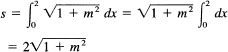
The base of the triangle is 2, the height is 2m, and we have, therefore, the hypotenuse we just computed.
Example 18.4-2
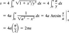
Find the circumference of a circle of radius a. We represent the circle in the form
![]()
We use the form for the arc length (18.4-5) and compute (using symmetry) four times the length in the first quadrant:
![]()
We must find y′. By implicit differentiation of the equation for the circle, we get
![]()
and the formula for the arc length becomes (using the equation of the circle)
which is what it should be.
We conclude that the definition we made for the length of a curve is reasonable. It assumes that at every point the derivative of the curve exists. At comers, we simply break up the curve into pieces each of which has a derivative in the interval (although the ends do not have a two-sided derivative). This is simply our usual (in this course) piecewise decomposition of curves into a finite number of pieces. We are now free to apply it to other functions, but we should still keep an eye on the results to be sure that they are reasonable. Beware of positive and negative lengths that cancel!
Example 18.4-3
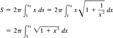
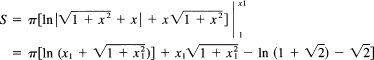
Consider the function y = In x. Suppose we want to measure its arc length, from x = 1. We have
![]()
and therefore we have
![]()
This integral is one of those we can hope to do, so we persist with
![]()
Make the usual transformation
![]()
to get rid of the radical (we could also use 1 + x2 = u2 instead if we wished). We have (dropping the limits for the moment)
between the limits 1 and x1. The result of some algebra is, on dropping the subscript on the upper limit,

At x = 1, we of course get 0. For large x we find that the increase in arc length is mainly from the first term and grows like x; and, since the In curve flattens out as x gets large, this is what we expect.
From this simple example we see the nature of the problem: the formula for arc length often leads to integrands that are hard, or impossible, to integrate in closed form. It is rare that arc length problems are nicely integrated. Thus for arc length problems we are often forced to numerical integration (Section 11.11). There is a collection of nice problems that have been found over the years and occupy the exercises in the standard textbooks. Few are of real importance beyond their use as exercises.
Example 18.4-4
Find the length of the four–cusp hypocycloid
![]()
We need ![]() for formula (18.4-5):
for formula (18.4-5):
![]()
Does this seem reasonable? If we look at the circle of radius a and compare it to the four–cusp hypocycloid (Figure 18.4-2), we see that the arc lengths should be much the same. The circle has 2πa length, which is close to 6a. Yes, the answer seems to be reasonable.
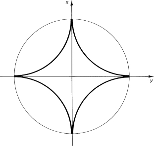
Figure 18.4-2 Four–cusp hypocycloid
Example 18.4-5
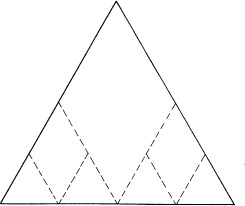
Lest you think that the length of a curve is a very simple idea, we give the following example of a sequence of curves each having a length that is the same fixed number; hence the sequence has this same limit. But the sequence aproaches a curve that has a different length!
Consider the line segment from 0 to 1. It has length 1. Erect an equilateral triangle on it (see Figure 18.4-3) whose two sides have a combined length of 2. Now “fold” the peak down to the line, making the path the edges of two equilateral triangles whose combined length is still 2. Now we fold down the two peaks to get the next curve of the sequence of curves. And so on. Each time the length of the broken path is 2, but the sequence of curves approaches the line segment. The limiting broken line has length 2, but it approaches the line of length 1.
You see what is wrong. Among other things, the limiting curve no longer has a derivative in the whole interval. In some sense the broken line is not approximating the straight line, although it is getting closer and closer, as measured by the maximum distance away, to the straight line. When we picked secant lines, then in the limit the secant lines approached the direction as well as the position of the curve. This is the
Figure 18.4-3 Arc length
essential difference between what we have been doing to approximate the arc length and this example.
1. In Example 18.4-3 makethe 1 + x2 + u2 substitution.
2. Find the arc length of y2 = 4x3 from x = 0 to x = x1.
3. Find the arc length of x2 = 9y3.
4. Find the length of the curve y = In cos x from x = 0.
18.5 CURVATURE AGAIN
We studied curvature in Section 8.4 by fitting a local circle to the curve and using the reciprocal of the radius of the circle as a measure of the curvature at that point. The formula for the curvature kappa was
![]()
Now that we have the concept of arc length, an alternative definition of curvature suggests itself; how fast does the angle of the tangent line change as a function of the arc length? This definition appears to be independent of the coordinate system and hence to measure something intrinsic to the curve itself. (When we studied the ellipse in Section 6.5, we had two different measures of the deviation of an ellipse from a circle, the eccentricity e and the ratio r of the two major axes of the ellipse.)
From Figure 18.5-1 we have
![]()
or
![]()
Figure 18.5-1 Curvature
The rate of change of the angle θ with respect to the arc length s is simply
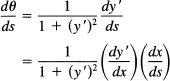
Since dy’ / dx = y″ and
![]()
we have
![]()
which is the same formula (almost) as before. This time the two definitions lead to essentially the same formula for computing the curvature and are therefore equivalent.
18.6 SURFACES OF ROTATION
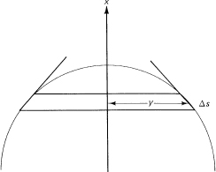
It is natural to pass from arc length to the surface S of a volume generated by rotating a curve around an axis. If we look at a picture of what an element of arc length does as it is rotated about a line, we see that it is closely approximated by the surface of a local tangent cone. In Figure 18.6-1, where the rotation is about the y-axis, we see that the surface is reasonably approximated by
![]()
where S is the surface generated and s is the arc length.
It is reasonable to test this idea on a cylinder (the result is obvious) and on a sphere.
Figure 18.6-1 Surface area
Example 18.6-1
Find the surface of a sphere of radius a. We rotate the circle
x2 + y2 + a2
about the x-axis (see Figure 18.6-1). By implicit differentiation we have y' = −x y. The formula for the surface, therefore,
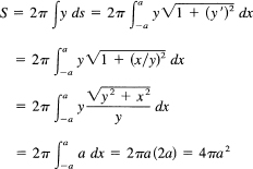
This checks our known result and gives us confidence in the method for finding the area of surfaces of revolution. A few other check cases are left as exercises.
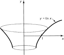
Example 18.6-2
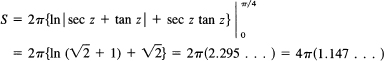
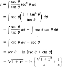
Suppose the curve y = In x is rotated about the y-axis. Find the surface generated by the segment between x = 1 and x = x1 (see Figure 18.6-2). The formula for the surface is
We naturally set x = tan θ; hence dx = sec2 θ dθ, and
![]()
which is an integral we have done (Example 16.5-8). Thus we have
Figure 18.6-2
![]()
to convert back to the variable x. We get
Example 18.6-3
Find the surface of the volume formed by rotating the curve y = sin x about the x-axis from x = 0 to x = π (Figure 18.6-3). We have immediately
![]()
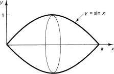
Figure 18.6-3
Set cos x= t then dt = −sin x dx and we have, on changing the limits,
![]()
Now set t = tan z; then dt = sec2 z dz, and the integral becomes
![]()
We know (from the integral table if no place else) that this is
which is slightly more than the surface of an enclosed sphere, 4π.
Example 18.6-4
Find the volume generated by rotating the area above y = −exp (−x) and below the positive x-axis about the y-axis (see Figure 18.6-4). We choose the cylinder method as shown (and use −y to get a positive volume):
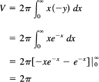
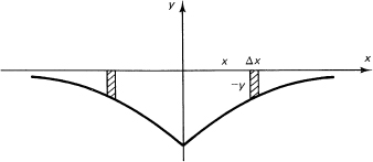
Figure 18.6-4
Note that the volume is finite, but that the surface, being at least as large as the whole plane, must be infinite! As they say, “You can fill the container full of paint, but you cannot paint the whole surface!”
This last remark shows some of the dangers of the immediate identification of the results of the mathematical model with the real world. The difficulty is that in mathematics the infinite surface generated by the rotating curve does not make a volume; it merely bounds a volume at best. You tend to think of the coat of paint as having some thickness (volume) and are led astray by the confusion between the mathematical and real models.
This is an interesting example, so we ask, “Can we make up another example of this type, this time having a container with finite maximum diameter, but having (necessarily when restricted to our class of functions) an infinite depth?”
Example 18.6-5
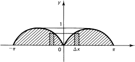
We begin with the reasonable choice of a curve to rotate about the y-axis as (0 < x ≤ 1)
![]()
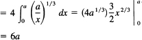
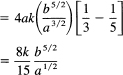
where we must require a > 0 to have the shape shown in Figure 18.6-5. The volume is given by
![]()
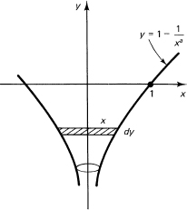
Figure 18.6-5
We compute dy, put that in the integral, and change the limits to the variable x:
provided we make 2 – a > 0 so that the improper integral will have the lower limit vanish. Thus the volume is finite when
0 < a < 2
and we cannot have the equality at either end, as you can show by considering those cases.
Next, we compute the surface area. We get
This integral is not easy to do. But all we need are bounds, so we think as follows: in the range (0 ≤ x ≤ 1) the factor x2 is not more than 1 while the other factor is large, especially near x = 0. Hence we drop the x2 term and write
![]()
and use this in the integrand for a lower bound on the integral. We get
![]()
provided 1 — a >0. For a < 1, it is easy to get a bound on the other side (since x2 < 1 and a2 < 1):
![]()
which will change the answer by a multiplicative factor of ![]() . Thus the surface area is infinite for 1 < a < 2, while for this range the volume is finite. Both the surface and the volume are finite for 0 < a < 1.
. Thus the surface area is infinite for 1 < a < 2, while for this range the volume is finite. Both the surface and the volume are finite for 0 < a < 1.
1. Check the formula for the surface of a cone.
2. Check the formula for the surface of a cylinder.
3. Find the surface generated by rotating y = exp(-x)(0 ≤ x ≤ 1) about the x-axis.
4. Find the total surface of the four-cusp hypocycloid x2/3 + y2/3 = a2/3 when rotated about the x-axis.
18.7 EXTENSIONS
When finding areas and volumes, we have taken rectangular strips, discs, and cylinders as our elements to sum. In the limit the sum passes over into the integral. Similarly, we took short line segments and strips of cones to find lengths of lines and surfaces of volumes of rotation.
But the integral is a limit of a sum, as was proved in great generality; although we began with areas, the elements in the sum were not tied to any specific quantities. This suggests that we can use any shaped sections we want in finding a volume (and other quantities). They can be similar shapes or not, as the following examples show.
Example 18.7-1
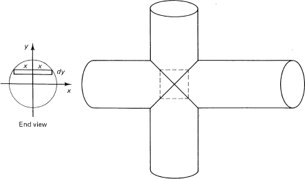
Two circular cylinders of the same diameter have their axes intersecting at right angles; find the common volume. The main problem is to visualize and draw the figure. Looking from the top of the intersecting cylinders, we get Figure 18.7-1, where, after some thought, we see the two lines of intersection meeting at right angles.
How to cut the common volume up into computable parts is the problem. After some thought we see that squares parallel to the top will lead us to elements of volume for which we can write a formula. Looking at the end view down one cylinder, we see that a side of a square is 2x; hence the element of volume is
(2x2) dy
Figure 18.7-1
where the variables are related by the equation
x2 + y2 = a2
The volume we want is, therefore,
![]()
Does the answer seem reasonable? The enclosing cube has volume 8a3, which makes the answer seem reasonable.
Example 18.7-2
A volume has a base that is circular,
x2 + y2 = a2
and the top is a line above the y-axis at a height h. The cross sections perpendicular to the y-axis are isosceles triangles with their bases on the circle. Find the volume (Figure 18.7-2).
The elements of volume are triangles with heights h, bases 2x, and thickness dy,
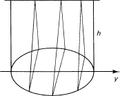
Figure 18.7-2
dV = hx dy
to sum. This leads to the integral
![]()
Put y = a sin θ to get rid of the radical.
![]()
and we recognize a Wallis integral. Hence the answer is
![]()
Thus the volume is one-half of the enclosing cylinder. A little thought about a cylinder, and the parts cut off, shows that this is indeed the answer.
Example 18.7-3
Find the volume of the ellipsoid
![]()
We cut the ellipsoid by planes parallel to the x—y axes. The section is
![]()
where z is a constant for the moment. We put this in the standard form for an ellipse:
![]()
The area of the ellipse is (see Example 18.3-3) tt times the product of the two semiaxes; hence the element of volume is
![]()
and the volume is given by
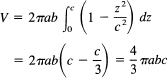
When a = b = c, we get the volume of a sphere; and when we think about it, the formula is just what it must be.
1. The cylinder x2 + y2 = a2 above the x–y plane is cut off by the plane z = x + a. Find the volume. Why is the answer obvious?
2. A volume has a base that is circular, x2 + y2 = a2, and cross sections are right triangles of sides h with the hypotenuse in the circle. Find the volume.
3. Do Example 18.7-2 when the base is an ellipse.
4. A volume has a base that is circular of radius a. Cross sections in a vertical plane perpendicular to the x-axis are parabolas centered above the x-axis with the top along a line c units above the x-axis. Find the volume.
5. A solid has square cross sections perpendicular to the x-axis with the bases on an ellipse. Find the volume.
18.8 DERIVATIVE OF AN INTEGRAL
It frequently happens that the integrand of an integral depends on a parameter c. In mathematical notation, we have
![]()
An example was the T(n) function (Section 15.11), where, since n can be any real, positive number, we write c in place of n:
![]()
where now c is a real number greater than 0. This gives a reasonable extension of the notion of the factorial to all positive real numbers.
It is natural to ask about the derivative of F(c) with respect to c in (18.8-1). To answer the question, we go back to fundamentals and write out the details of the four-step process. At the third step, we have
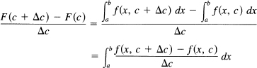
By the mean value theorem (Section 11.7) applied to the function f(c), the integrand has the value
![]()
for some θ in the interval from c to c + ![]() c, provided there is a continuous finite derivative of f(x, c) with respect to c in the whole interval [a, b]. The
c, provided there is a continuous finite derivative of f(x, c) with respect to c in the whole interval [a, b]. The ![]() c cancels out
c cancels out
of numerator and denominator. Now when we let ![]() c → 0, the left side approaches the partial derivative, and the integrand approaches its partial derivative. Hence we have the formula
c → 0, the left side approaches the partial derivative, and the integrand approaches its partial derivative. Hence we have the formula
![]()
provided ∂f/∂c is finite and continuous in the finite interval [a, b]. Why all these conditions? Some come from the hypotheses of the mean value theorem, and some come from the fact that we want a bound on the final integrand that is uniform in the interval lest at some place the values become unbounded. Finally, unless the interval is finite, we may be facing a situation where we have an error that is zero times an infinity, and the indeterminate value may not be zero. In loose words, you can differentiate under an integral sign with respect to a parameter provided the derivative is continuous in the interval of integration. In practice, you had best avoid improper integrals in both the original integral and in the derivative integral, or else be prepared to examine things much more closely than we have done.
Example 18.8-1
Consider the known integral
![]()
If we differentiate the left side with respect to c, we get
![]()
We can, of course, differentiate again and again, obtaining the integrals
![]()
The simple formula (18.8-3) allows us to generate new integrals from old ones (which contain a parameter) by the direct process of differentiation with respect to the parameter. Indeed, there is an art of changing variables to introduce the proper parameter into the integral so that the differentiation will lead you to the integral you want to solve. It is a powerful method for generating a table of integrals.
Example 18.8-2
Consider the integral
![]()
Differentiating once with respect to the parameter a and multiplying through on both sides by (–1), we get
Differentiating again we get (again multiply by —1)
![]()
and in general we get from the (n — l)th derivative
![]()
which is the ![]() (n) function of Section 15.11 and (18.8-2). What was obtained there by integration by parts is here found by simple differentiation. We ignored the warning about improper integrals, because in this case it is easy to start with a finite range, get the answer, and then let the range go to infinity.
(n) function of Section 15.11 and (18.8-2). What was obtained there by integration by parts is here found by simple differentiation. We ignored the warning about improper integrals, because in this case it is easy to start with a finite range, get the answer, and then let the range go to infinity.
Example 18.8-3
Consider the indefinite integral
![]()
Differentiate with respect to a:
![]()
where we have added the constant of integration, which vanished when we differentiated but is needed for indefinite integrals. Again, what you might have obtained by integratioi by parts is found by differentiation.
Since the method is clearly so powerful, we should look a bit closer and answe the question of partial differentiation when the parameter can also occur in the limits
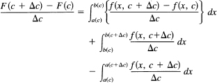
Example 18.8-4*
Suppose we have the integral
![]()
and want to differentiate with respect to c. One suspects how the formula will go, but to be safe we will go through the details of the four-step process. It is only algebra with nothing really new in the whole process, just the use of old ideas in a new situation.
![]()
But this can be written as the difference of two integrals over the common range plus the pieces over the extra ranges:
In the first integral we apply the mean value theorem (Section 11.7), and in the second two we apply the mean value theorem for integrals [Section 13.3: the average over an interval is some value of the integral in the interval with the g(x) = 1]:
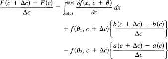
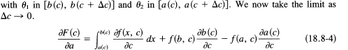
This is more or less what you would expect from the function of a function rule for differentiation, plus the rule for differentiation of an integral with respect to its limits. If we write the indefinite integral of f(x, c) as F(x, c), then the integral would be
![]()
and you see the derivative emerging. It is futile to try to remember the formula in detail; it is easy to remember if you ask, “What does it say?” It says that you differentiate with respect to the parameter wherever it occurs; in the integrand you copy the result with the partial derivative (as before), but for the parameter in the limits, remembering the fundamental theorem of the calculus, you get the integrand at the limits times the derivatives of the limits; the upper limit of course is positive and the lower is negative. Thus it includes the fundamental theorem of the calculus that the derivative of an integral with respect to the upper limit is the integrand.
EXERCISES 18.8
1. Given the integral ![]() , differentiate with respect to a once to get a new integral.
, differentiate with respect to a once to get a new integral.
2. Use the formula for ![]() to get new integrals.
to get new integrals.
3. The integral leading to the arctangent seems difficult to differentiate repeatedly. Note that, using complex numbers, l/(c2 + x2) can be factored into complex linear factors and you are led formally to the In of complex numbers, whose formal derivatives are easily found.
4. Discuss introducing a parameter by a change of variables and then using it to get new integrals.
18.9* MECHANICS
We earlier noted that the calculus was developed in terms of mechanics. It is mainly the words that are changed between mechanics and statistics, as we will now show.
We have already discussed velocity (Section 9.3) and acceleration (Section 9.4). The next application is to the center of gravity. At first we imagine a solid of uniform density (which for convenience we can take as 1) and ask where all the mass could be put so that it is equivalent to being at one single point. This is the same question as the mean value of a distribution. We can take the origin of the coordinate system at any place we please and measure the distance to the typical unit of mass from that point. This must be divided by the total mass (in probability theory the total probability was 1, so it was ignored). The formula for the x coordinate of the center of gravity is
![]()
We can think of dV = dx dy dz, and m as the element of mass. We will then be summing an element to get a row, the rows to get a plane, and the planes to get the volume. This will be studied in the next chapter; meanwhile we will only use elements of volume in the cases where we can get a suitably shaped element of volume directly. There are similar formulas for the other coordinates of the center of mass. This is also called the center of gravity if you prefer. Notice that the mass or density will drop out, and the result is independent of units used except for the distance unit. We can therefore drop the quantity m from the formula for the center of gravity if we wish, provided it is homogeneous material.
If the density is not uniform, then we merely have a weighted average in both the numerator and denominator to compute.
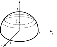
Example 18.9-1
Find the center of mass of a uniform hemisphere of radius a. We first pick the coordinate system at the center of the sphere. We have the equation
![]()
and use the upper half-plane as the hemisphere. The center in x and y lie on the axis of symmetry, and it is only the z coordinate that is needed. The formula, using discs as in Figure 18.9-1, is
![]()
Figure 18.9-1 Hemisphere
where we have used the fact that we know the volume of the hemisphere. When we recognize that we are using the circular symmetry found by rotating the circle
x2 + z2 = a2
about the z-axis, we can use the fact that
x2 = a2 − z2
The integral becomes
This seems like a reasonable result; the average of the mass is slightly below the midpoint on the z-axis.
Another mechanical concept is the moment of inertia about a line through the center of mass. This is exactly the same as the variance (about the mean) in statistics, again remembering to divide by the total mass. In place of the first moment used for the center of gravity, we use the second moment about the axis of rotation.
Example 18.9-2
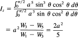
Moment of inertia of a sphere. The moment of inertia of a sphere rotating about, say, the z-axis can be found by cutting the sphere up into cylinders (Figure 18.9-2) and noting that all points on the cylinder have the same distance from the axis of rotation. Thus the ratio of the second moment divided by the volume (mass) gives the moment of inertia about the z-axis:
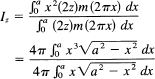
Set x = a sin θ, dx = a cos θ dθ, to get
Another concept that is often used in mechanics is the center of pressure, say on a dam. We picture the cross section of the water against the dam as a parabola (Figure 18.9-3). The pressure of the water is proportional to the mass in a column above the element shown. Thus the pressure is the first moment about the top of the water. Nothing else is new.
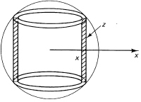
Figure 18.9-2 Moment of inertia of a sphere

Figure 18.9-3 Pressure on a dam
Example 18.9-3
Using the parabolic shaped dam
y = ax2
we have the total pressure as
![]()
where k is some suitable constant (see Figure 18.9-3). We can either substitute for the x values the corresponding values in y or else change from y to x as the independent variable. We do the latter.
You see that, if you understand the physical concepts, then it is a matter of using the same sort of calculus as you have been doing to get the answers. Of course, the details may be messier, but the calculus ideas are the same. If you do not understand the field of application, then it all becomes hazy to say the least! To use mathematics successfully, you need to know what you are talking about, both the mathematics and the field of application.
1. Find the center of gravity of a cone.
2. Find the center of gravity of half an ellipsoid of revolution.
3. Find the moment of inertia of a cylinder rotated about the axis of symmetry.
4. Find the moment of inertia of a cone rotated about its axis ofsymmetry.
5. Find the force on a semicircular dam filled to a height h.
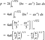
18.10* FORCE AND WORK
Force is another topic that arises in mechanics. Forces play a central role in mechanics. Any force can be broken up into a pair of forces in different directions, such that the original force is the diagonal of the parallelogram formed by the two derived forces (Figure 18.10-1). See Section 9.4.
Newton’s law
f = ma
connects mass with weight. In a gravitational field, such as the earth, the weight of an object is the mass times the gravitational force, usually labeled g.
Force applied through a distance is called work, the force times the distance being the measure of the amount of work. If the force is constant and the motion is in a straight line, then the computation is easy. But if (1) the mass varies with time,
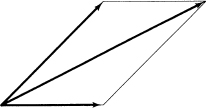
Figure 18.10-1 Parallelogram of forces
as in a rocket using up its fuel, (2) the force varies with position, or (3) the motion is along a curved line and the motion is not necessarily in line with the force, then the calculus is necessary. Notice that work can be positive or negative, meaning you put in work or get it out of the system studied. It is also true that the amount of mass moved, as well as the distance it is moved per unit time, may vary as the task proceeds.
Example 18.10-1
The force exerted by a spring, when displaced from its equilibrium position (of no force), is proportional to its displacement (extension) x (Figure 18.10-2). This is known as Hooke’s (1635–1703) law. Let the constant of proportionality be k; that is,
f = kx
If the end is moved from x = 0 to x = a, how much work is done?
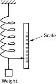
Figure 18.10-2 Spring scale
We have to compute
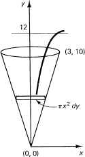
Example 18.10-2
How much work is required to lift the water (one cubic foot of water weighs 62.5 pounds) in a cone shaped as in Figure 18.10-3 to a level 2 feet above the rim? We take an element of volume it x2dy, and since the weight is 62.5 lb/ft3, we merely multiply by 62.5, and integrate it when multiplied by the distance the element of volume is moved; that is, 2 + (10 – y). We have
![]()
We need to get x in terms of y, and from the figure x = 3y/10. Hence we have
Figure 18.10-3 Work
where we have kept the weight separate so you can follow it easily.
Example 18.10-3
Show that the work done in emptying a volume is the same as moving the center of mass through the distance. We simply write out the two formulas, noting how the density term arises, and see the equivalence. Thus there is little new in the matter of emptying volumes of liquid.
1. Find the work done in emptying a hemispherical bowl when the water is lifted to a height h.
2. How much work is done when a hemispherical bowl is drained through a hole in the bottom?
3. How much work is done in bailing out a 1-foot cube of water when the water is lifted just over the upper edge of the cube?
18.11* INVERSE SQUARE LAW OF FORCE
Many phenomena, for example the force of gravity, the force between electrostatic charges, and light intensity, have an inverse square law
![]()
where d is the distance involved. For example, the force of gravity is given by
![]()
where G is a universal constant (depending on the units used to measure things), m1 and m2 are the two attracting masses, and d is the distance between them.
Example 18.11-1
Suppose you have wire of uniform density in the shape of a semicircle of radius a. What is the force on a unit of mass located as shown in Figure 18.11-1?

Figure 18.11-1 Semicircular wire
Each element ds along the circumference has mass proportional to a ds. The component of force along the axis is multiplied by cos 0/2 (since the angle is half the central angle). The distance comes from the law of cosines:
![]()
The element of force due to the element of mass along the circumference has some constant of proportionality, say k, and is given by
![]()
The total force is, therefore,
![]()
We use the half-angle formula on the denominator and symmetry to get
What is the attraction of a rod of length 2a on a point opposite its center and at a distance h? We draw Figure 18.11-2. Remember that the force is a vector, and by symmetry we see that only the component in the direction perpendicular to the rod will matter. The square of the distance to an element of mass of the rod is
x2 + h2
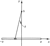
Figure 18.11-2 Attraction of rod
We must take the cosine component of the force:
![]()
and sum this up for each element dx. We have (k is the density of the rod)
![]()
Set x = h tan θ then dx = h sec2 θ dθ, and
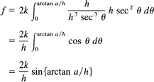
From Figure 18.11-2, we see that the answer is
![]()
which seems to be reasonable.
1. Find the force exerted by a wire ring on an element of mass located on the axis of the circle at a distance b away.
2. Using the result of Exercise 1, find the force of a disc on an element of mass on its axis.
3. Find the increase in velocity of a point mass in falling through a gravitational field from bio a. Let b approach infinity. This is also the “escape velocity” and can be evaluated from the gravitational force at the surface of a planet and the radius of the surface. For the earth, it is about 6.9 miles per second (neglecting all such details as air drag, rotational effects, etc.).
18.12 SUMMARY
In this chapter, now that we have a larger class of functions we can handle, we first reviewed a few of the standard applications of the calculus. Then we examined a number of new, but at this point not essentially difficult, applications. They depended mainly on a knowledge of the field of application. When you know your field well, then it is not as difficult as it may at first seem to make new applicaitons of the calculus to your field. It is necessary to practice converting word problems to mathematical formulas and the reverse, from the mathematics to get back to the words. By practicing these two steps, you prepare yourself for when the time comes for you to contribute to the advancement of knowledge.
Most of the material should be learned not in terms of the results, but in terms of the approach. Thus the elementary triangle, from which we derived the arc length and later the formulas for surface of revolution, is the basic concept and can hardly be called sophisticated or difficult. It is interesting that the two apparently different notions of curvature should turn out to be the same thing (almost).
Section 18.7, devoted to extensions, is based on the generalization we derived of the fundamental theorem that connected the summation of elements of any general form with the corresponding integral. It is another example of learning what the general formula says and then being willing to apply the generality, rather than being limited to the specific cases you began with. Thus you see, again, the value of generalization and the power that comes when you have investigated a result to understand essentially what it does and does not depend on. The author is convinced that (1) only by making these generalizations your own can you hope to make significant contributions to your chosen field, and (2) that it is often only this step that significantly advances a field. The world is rapidly changing, and the applications of the calculus, probability, and statistics will also probably be greatly extended and changed within your lifetime; so if you are to play a part in this process, it is wise to master not only the details, but the underlying assumptions that produced the current version of mathematics.
The differentiation of an integral is a natural question and generalizes the fundamental theorem that the derivative of the integral with respect to the upper limit gives the integrand at that point. We investigated the problem in some detail to familiarize you with the processes of abstraction, generalization, and extension. These are the heart of mathematics; these are what the book is really about.
The specific applications to mechanics, force, work, and inverse square law are interesting applications of mathematics and have shaped mathematics extensively; yet they are only the applications, not the essence of mathematics. We avoided the applications to probability and statistics in this chapter, but similar examples could be found easily.