23.1 WHAT IS A DIFFERENTIAL EQUATION?
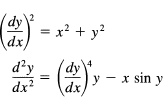
A differential equation is a relationship among x, y, y′,y″, … y(n), where the primes are derivatives of the function y = y(x). For example,
are differential equations. These are ordinary differential equations because they involve only ordinary derivatives. If there were partial derivatives, then the equations would be called partial differential equations, but we will not study these.
The order of a differential equation is the order of the highest derivative appearing. Thus the first example is of first order and the second is of second order. The degree of the equation is the power of the highest derivative appearing. The first is of second degree and the second is of first degree.
We have already studied the special case of
![]()
and found that the solution (the indefinite integral) involves an arbitrary additive constant. In the more general case of a first-order first-degree equation
![]()
the solution will also involve a single arbitrary constant, but it need no longer be an additive constant C. In this chapter we will look mainly at first-order differential equations, but we will look briefly at two special cases of second-order equations of the form
![]()
whose solution will have two arbitrary constants in the general solution. The topic of differential equations is so vast that we can take only a very limited look at it in this book.
23.2 WHAT IS A SOLUTION?
There are three different kinds of answers we can give to the question, “What is meant by the solution of a differential equation?”
First, there is what might be called the algebraic answer, which is simply “A solution is a function that when substituted, along with its derivatives, into the equation exactly fits the equation.” As an example, we have
![]()
where C is an arbitrary constant. Direct differentiation and substitution into the differential equation gives an identity in x. Another example is
![]()
where both C1 and C2 are arbitrary constants. Again it is easy to check that this is a solution. In both cases it is a matter of simply differentiating the solution and then substituting into the differential equation to verify that you have a solution. In this respect it resembles verifying that you have found the right integral; you simply differentiate and note that you have the integrand.
Second, there is the geometric answer, “The solution of a first-order differential equation is a curve along which the slope at any point is exactly the derivative at that point as given by the differential equation.” (Similar results apply for higher-order equations.) This introduces the idea of the direction field of a first-order differential equation, which is a picture at each point of which the slope element (as sketched in the Figure 23.2-1) has slope given by the differential equation. An example is
![]()
We could take a close mesh of points, compute the slope at each point, and then draw the corresponding curves through the points such that at each point the curve has the indicated slope. Roughly, we would get a curve with the appropriate slope through each point of the picture (Figure 23.2-1).
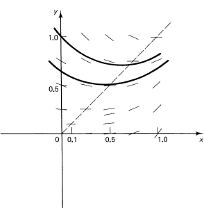
Figure 23.2-1 Direction field, y′ = x2 − y2
In this approach it is much easier, generally, to locate the curves along which the slope is a constant, the isoclines (iso-, same; clines, slope). For the above differential equation, the isocline curves are the hyperbolas
x2 – y2 = c
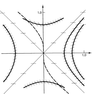
The slope along each of these curves is c. Figure 23.2-2 shows the direction field, and some possible solutions to the equation are sketched in.
In general, points on the isocline along which y′ = 0 represent local extremes of the solutions. In the above example, these curves of maxima and minima are the two straight lines
![]()
If you differentiate the differential equation to get the second derivative and then set this equal to zero (and eliminate the first derivative, if it occurs, by using the original differential equation), you get the curves along which the inflection points of the solution must lie. In the example this gives
![]()
Divide out the 2 and eliminate the y′ to get the curve
![]()
This curve is indicated by the dotted line in Figure 23.2-2.
Figure 23.2-2 Isoclines
There is a third answer to the question, “What is a solution?” The differential equation describes the local conditions that the function must obey at every point; the solution is the global answer. Thus solving a differential equation means going from the local description to the global description.
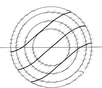
We have said that through each point in the plane there is a single solution, but this can be misleading. Consider the differential equation
![]()
Using isoclines it is easy to make a crude sketch of the direction field (Figure 23.2-3). We see immediately that outside the circle of radius 1 there is no solution since the slope is imaginary. The solution to this differential equation is confined to a limited area of the plane.
Sketch the direction fields and find the curve of max-min.
1. y′ = 1 – x2 – y2
2. y = xy′ + (y′)2
3. y′ = x/(x + y + 1)
4. Find the curve of inflection points of y′ = x2 + y2.
Figure 23.2-3 ![]()
23.3 WHY STUDY DIFFERENTIAL EQUATIONS?
A differential equation is a local description of how a system changes. Given that a system is in some state now and subject to a given set of “forces,” what is the immediate response of the system? When we solve this, we get the global description of the corresponding phenomenon.
As we currently understand the world, many of the things we are interested in fall into the general pattern of being expressed by a differential equation. In astronomy the planets are subject to various forces, chiefly gravitational. The planets have a present position and present velocity, and the gravitational interactions, via Newton’s laws of motion, describe the main part of the evolution of the solar system. Newton’s law
![]()
(where f = force, m = mass, and s = position) is a differential equation. Similarly, in physics and chemistry the basic laws (as we currently understand them) connect the present state of the system with the immediate future state. Even in biology we have such simple examples as the following: with an adequate food supply the growth of a bacterial colony is proportional to its size, or
![]()
where S = S (t) is the size of the colony at time t, and k is the constant of proportionality. In the social sciences we may have a situation that is more or less stable; then at a given date a new law becomes effective. As a result, the social (or economic) system reacts to the new conditions by making local changes. Thus the corresponding model of the social system is apt to be a set of differential equations connecting the variables and their rates of change.
Each field of application requires a knowledge of the details of the field, the rules (laws) of what will arise in the immediate future from the given state and given forces. Mathematics will seldom supply much help (beyond dimensional analysis) with the basic formulation of the model you are studying; but once the model is formulated, mathematics can tell you how the model would evolve, and hence (insofar as the modeling you have done is relevant and accurate) you will be able to anticipate the consequences that would occur if the proposed model is followed. In particular, in the social sciences it is necessary to model systems rather than experiment on real live models that include humans themselves. Modeling, or as it is often called, simulation, is the answer to the perennial question, “What if …?” Often differential equations will aid in answering such questions (provided you have made a relevant model).
23.4 THE METHOD OF VARIABLES SEPARABLE
The easiest differential equations to solve, beyond mere integration, are those in which the variables can be separated as in the following examples.
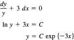
Example 23.4-1
Solve the differential equation
![]()
We write y′ as dy/dx and then separate the variables (using differentials) to obtain two integrals. The detailed steps are shown below.
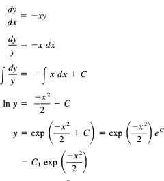
where we have written the constant ec = C1.
The constant of integration for differential equations no longer appears as an additive constant; it may appear almost any place and in any form. The disguise of a constant can cause the student trouble until it is realized that both results for the differential equation
![]()
whose solutions are
![]()
are the same; they differ by the meaning of the C. The C in the second solution is merely
C + a2
of the first solution. Both are constants, so for suitable choice of C in either case you can get the same solution.
Example 23.4-2
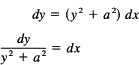
Integrate the differential equation
![]()
We have
Integrating both sides, we get
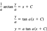
This is a one-parameter family of solutions of the differential equation. Often only one particular solution is wanted. We are in a position similar to that for the method of undetermined coefficients; we must impose the proper number of conditions to determine the unique solution. In this case, suppose we want the solution through the origin (0, 0). We then have
![]()
It is natural to pick C = 0, although other values such as C = kπ/a will give the same result. The particular solution is, therefore,
y = a tan ax
Direct substitution will verify that this fits both the equation and the assumed boundary (or initial) condition.
Integrate
![]()
Taking slightly larger steps, we get in sequence
where we have calmly written ec as a constant also labeled C. We could give one of the constants a subscript to distinguish the multiple use of the same symbol, but it is rarely done in practice. You simply replace any convenient form of a constant by C (being slightly careful not to confuse yourself in case there are several different Cs).
If we tried to find a solution to this differential equation that passes through the origin, we would have
0 = – 1
and the constant C does not appear. This, plus the simple fact that the equation is a contradiction, shows that there is no solution that passes through the origin. If we picked the point x = 1, y = 0, we would have
![]()
and hence C = e1/2 and the particular solution is
![]()
Example 23.4-4
Integrate
![]()
We separate the variables:
in the general solution of the differential equation. Direct substitution to check the solution gives
If we reduce the problem to integrals, then even if the integrals cannot be done in closed form we regard the solution of the differential equation as having been found. In this method of separation of variables, it is sufficient, in theory, to write out the integrals. In practice, of course, the integrals must be done, but that is now a technique that you have presumably mastered and to give the details at this point would obscure the ideas of how to solve differential equations. However, in the exercises you are expected to work out the integrals to give you further experience in this art. But do not confuse the basic simplicity of the method of solution with the complexity of some of its steps.
Example 23.4-5
The astronomer Sir John F. W. Herschel (1792–1871) gave the following derivation of the normal distribution. Consider dropping a dart at a target (the origin of the coordinate system) on a horizontal plane. We suppose that (1) the errors do not depend on the coordinate system used, (2) the errors in perpendicular directions are independent, and (3) small errors are more likely than large errors. These all seem to be reasonable assumptions of what happens when we aim a dart at a point.
Let the probability of the dart falling in the strip x, x + Δx be p (x), and of falling in the strip y, y + Δy be p(y) (see Figure 23.4-1). Hence the probability of falling in the

Figure 23.4-1
shaded rectangle is
![]()
where r is the distance from the target to the place where the dart falls. From this we conclude
Now g (r) does not depend on θ; hence we have
![]()
But we know that
![]()
and we can write
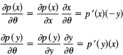
This gives
![]()
Separating variables in this differential equation, we get
![]()
Both terms must be equal to a constant K since x and y are independent variables. This is a crucial step, so think this through! Changing either variable cannot change the other term; hence each term must be a constant. The equations are essentially the same, so we need only treat one of them. We have
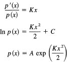
But since small errors are more likely than large ones, K must be negative, say
![]()
(thus we get the formula in the standard form). This means that
![]()
The condition that the integral of a probability distribution over all possible values must total to 1 means that we can determine the constant of integration A to be
which is the normal distribution with mean zero and variance σ2.
This derivation is seductively innocent, but in the final analysis the normal distribution rests on arbitrary assumptions. The name, normal distribution, implies that somehow you should “normally” expect to see it, but often random variables come from other than normal distributions. Furthermore, experience shows that, while the main part of the distribution often looks like a normal curve, the tails of the distribution may be either too small or too large. There are other sources of the normal distribution. For example, the central-limit theorem, which we do not prove here, states loosely that the sum of a large number of small independent errors will closely approximate the normal distribution. We saw something like this in Example 12.6-1.
Integrate the following using the variables separable method.
1. y′ = c
2. yy′ = x
3. xy′ = y
4. y′ = xy
5. xy′ = (1 + x)(1 + y)
6. y′ = xy − x −y + 1
7. y′ = y lnx
8. y′ = xmyn
9. Show that the sum of 12 independent random variables, from a uniform distribution ![]() , minus 6 has mean zero and variance 1.
, minus 6 has mean zero and variance 1.
23.5 HOMOGENEOUS EQUATIONS
There is a large class of differential equations that can be solved by reducing them to variables separable. They are of the form of homogeneous equations, where by “homogeneous equations” we mean that all the terms are of the same degree in the variables. Thus the terms
![]()
are all homogeneous of degree 2. The test is that, on substituting xt for x and yt for y, the variable t factors out of all the terms and emerges, in this case as t2, multiplying the original expression.
If the equation is homogeneous, then the change of variable, y = vx, to the new variable v in place of y will produce an equation whose variables are separable, and we are reduced to the previous case.
Example 23.5-1
Integrate
![]()
This is a homogeneous equation of degree 1. Set y = vx and get

An alternative expression, and one that you might prefer, is to solve for y. We have
Example 23.5-2
Integrate
![]()
for a continuous function f(y/x). We make the usual change of variables
y = vx
to get
![]()
and separate variables
![]()
and we have reduced the problem to quadratures.
Unless we are given a particular function f(y/x), we can go no further.
It is worth noting that the use of polar coordinates
x = r cos θ, y = r sin θ
will also lead to a variables separable equation, and at times the use of polar coordinates may shed more light on the situation than the use of the more compact change y = vx.
Example 23.5-3
Using the equation of Example 23.5-1, we get
![]()
and the equation becomes
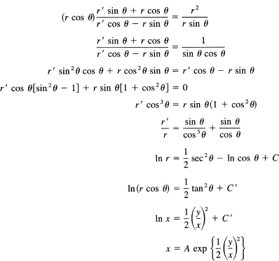
as before. In this case the amount of algebra is distinctly larger than before.
Solve the following equations.
1. y′ = (x + y)/x
2. y′ = xy/(x2 + y2)
3. y′ = (x2 + y2)/2x2
4. (x + y)y′ = x − y
5. (2x2 − y2)y′ + 3xy = 0
23.6 INTEGRATING FACTORS
It is evident that we can write a first-order, first-degree, differential equation in the form
![]()
Sometimesthis can be put in the form of the derivative of a function of the variables x and y. For example, if we had
![]()
then multiplying through by x gives
![]()
and this is the derivative of
![]()
When we have the situation where the equation is the derivative of a function, we call it an exact differential of the function, and we can solve the problem.
Example 23.6-1
Solve
![]()
This is the derivative of
![]()
and we have the solution. (It could also have been solved by the variables separable method.)
Example 23.6-2
Solve
![]()
This can be written in the form
If you want the particular solution passing through the point x = 0, y = 1, then you must have
1 = C
Therefore, the particular solution through (0, 1) is
![]()
Often the equation as it stands is not an exact derivative of some function, but by multiplying by a suitable function it can be made exact. Such a function is called an integrating factor.
Example 23.6-3
Solve xy’ + ny =f(x). A little study suggests the product form; hence we need to multiply through by xn-1 to get
![]()
We now have
![]()
and integrating both sides gives us
![]()
as the solution.
Example 23.6-4
Integrate
![]()
Rewriting this in the form (multiply by cos x)
![]()
leads to
![]()
and integrating this we get
![]()
![]()
Example 23.6-5
Integrate
![]()
The difference in signs between the two terms on the left suggests a quotient, so we divide by x2 to get
![]()
from which we get

Finding an integrating factor is evidently an art requiring experience with derivatives so that you can imagine how to construct a function which upon differentiation will lead to your expression. There is not a unique integrating factor, and different ones can lead to different forms of the answer.
The condition that there exists an integrating factor depends on the fact that the exact differential equation must come from the solution
![]()
by differentiation. Hence, if the integrating factor is called r(x, y), then
![]()
means that
![]()
This is only slightly useful in searching for an integrating factor.
When we have the differential equation in the exact form, it remains to find the solution. Since we know
![]()
if the derivatives exist and are continuous, then
This provides us with a method for solving the equation when it is an exact differential. Integrate
![]()
inserting a function of y for the arbitrary constant. Substitute this into
![]()
and determine the arbitrary function of y. The solutions is then
u = C
By symmetry we could, of course, reverse the order and integrate with respect to x first.
Example 23.6-6
Integrate
![]()
We have
![]()
which shows that the equation is exact. From
![]()
we have, upon integration with respect to x,
![]()
Then we have
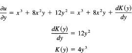
The solution, is therefore,
![]()
Integrate the following:
1. xy′ + 4y = 3
2. xy′ − 4y = 3
3. y + ctn xy′ = cos x
4. (x + y)2)dy + (y − x2)dx = 0
5. (xy + 1)/y dx + (2y − x)/y2 dy = 0
6. (4y2 − 2x2)/(4xy2 − x2)dx + (8y2 − x2)/(4y3 − x2y)dy = 0
23.7 FIRST-ORDER LINEAR DIFFERENTIAL EQUATIONS
An important class of differential equations has the form
![]()
This equation is called a linear first-order differential equation. It is linear in y and its derivatives and is of first order. We look for an integrating factor, and after a few moments we see that if we multiply through by
![]()
we will have
![]()
This can be written as
![]()
Upon integration, this becomes
![]()
where we have had to change to the dummy variable s in the integral on the right-hand side to avoid confusion between what are the variables of integration and of the problem. Of course, as indicated, the variable x is to be put in the integral in the exponent when it is done.
We have reduced the problem of solving first-order linear differential equations to a matter of doing two quadratures (ordinary integrations), as they are called. We conventionally regard the problem as solved as a problem in differential equations. Of course, in practice a great deal more work may be required to get the solution in a useful form. The habit of regarding the problem in differential equations as solved when it is reduced to quadratures is an example of “divide and conquer”—attack one phase of the problem at a time. The general solution looks messy, but when we can solve ∫[P(x) dx] in closed form, it often makes things look simple. We do not try to remember the form of the result and substitute into it, but rather remember the method of derivation and repeatedly use it. It is the methods of doing mathematics, rather than the results, that are important.
Example 23.7-1
Integrate
![]()
We first put it into the standard form
![]()
We have
![]()
and
![]()
Hence
![]()
Multiply the standard form through by this integrating factor to get
![]()
Integrate both sides to get
![]()
Or
![]()
At this point we check that we have no errors by differentiating and manipulating the terms that emerge.
as it should.
Example 23.7-2
Integrate
![]()
The integrating factor, upon integrating P(x) = 2x, and taking its exponential, is
![]()
and we have
![]()
and we can now do the indicated integration on the left to get
![]()
The integral on the right cannot be done in closed form.
An alternative approach to first-order linear differential equations, and one which has the great advantage that is generalizes to nth order equations, is the following. Given the equation
![]()
we first study the homogeneous equation (the right-hand side set equal to zero)
y′ + P(x)y = 0
This is easily solved as follows:
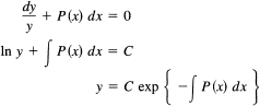
Suppose, next, that we can find one solution Y(x) of the original complete equation; that is, we can find a particular y(x) such that
Y′ + P(x)Y = Q(x)
Then the general solution of the complete equation is
![]()
We check this by substitution into the original equation:
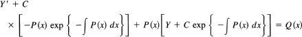
The terms with the constant C term all cancel out, and the other terms in Y also cancel since they are a solution of the complete equation. We see that one single solution of the complete equation causes the right-hand side to cancel, leaving the constant of integration term to satisfy the homogeneous equation.
How do you find the supposed solution Y(x)? By guessing! Or any other method you care to use (for example, the method of variation of parameters to be studied in Section 24.4).
Example 23.7-3
Consider the equation
y′ + 3y = x2
It is reasonable to guess the form for a solution of the complete equation as
Y(x) = ax2 + bx + c
This gives, on putting it into the given differential equation,
(2ax + b) + 3(ax2 + bx + c) = x2
Equating coefficients of like powers of x, we have

Their solution is easily found to be
![]()
hence the particular solution is
![]()
The solution of the homogeneous equation
y′ + 3y = 0
is
The general solution of the complete equation is therefore
![]()
Example 23.7-4
Consider the equation
y′ + y = sin x
We naturally try for the particular solution Y(x):
y(x) = A sinx + B cos x
Hence we get
A cos x − B sin x + A sin x + B cos x = sin x
and equate like terms in cos and sin (they are linearly independent functions). We get the equations
A + B = 0
-B + A = 1
The solution is A = ![]() , B = –
, B = –![]() , so we have
, so we have
![]()
We have now to solve the homogeneous equation
y′ + y = 0
It is easy to get the solution
y = Ce-x
So the complete solution is
![]()
This is easily checked by direct substitution.
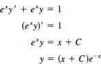
Example 23.7-5
Integrate
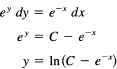
y′ + y = e-x
We try for the particular solution
Y(x) = Ae-x
This leads to
A(-e-x) + Ae-x = e-x
which is a contradiction, 0 = e -x. Next we try, after some thought,
Hence we get A = 1, and the particular solution is
Y(x) = xe-x
The homogeneous equation
y′ + y = 0
has the solution
y = Ce-x
So the general solution of the complete equation is
y(x) = xe-x + Ce-x = e-x(x + C)
This shows indirectly why the original trial for the particular solution failed; the trial solution was a solution of the homogeneous equation. When this occurs, putting an extra factor of x in front will lead to a solution.
Differential equations usually arise from the nature of the original problem, but at times they are “manufactured” by the mathematician, as the following example shows.
Example 23.7-6
Suppose you have the integral, as a function of the parameter a,
![]()
After other approaches fail, we try to find a differential equation for the function F(a) (assume for the moment that a > 0).
![]()
Now for a ≠ 0 set x = a/t. The integral becomes
![]()
Hence we have the differential equation
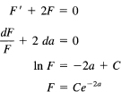
for a > 0. But we see immediately from the original problem that this form also applies for − a (we need to avoid a = 0). Hence the solution is of the form
F(a) = Ce–2|a|
To find C, we use a = 0, which is an integral we already know.
![]()
We have, therefore, the solution for the integral:
![]()
We seem to have the answer, but we made the transformation for a ≠ 0, and we used the value a = 0 to determine the constant of integration. So we need to examine the process a bit more closely.
Did the integral for the derivative F’(a) converge? Well, as x → 0 the exponent for a ≠ 0 beats out the factor 1/x2. But let us look at the integrand more closely. The main effect is the exponent, so we study the function (the exponent only)
![]()
The maximum occurs when the derivative
![]()
This occurs at ![]() this point the original integrand has the value
this point the original integrand has the value
e-2a
and while this is not the maximum of the integrand [only of the exponential factor g (x) that was used to locate the position], it gives us a clue as to the shape of the integrand. (We could find the actual maximum if we wished, but it is not worth the trouble as we want to understand the shape of the integrand, not its detailed behavior.) As a → 0, this tends to peak up, as does the true maximum of the integrand. Thus the peak of the integrand narrows as a → 0, and the integral approaches the limiting area ![]() . We are uneasy to say the least. Looking at the integrand at x = 0, we see that
. We are uneasy to say the least. Looking at the integrand at x = 0, we see that
![]()
The integrand value at x = 0 has a discontinuity as a → 0. However, the width of the peak approaches 0, and we think that we are safe in assuming that the integral itself is continuous at a = 0. We see from this one example the need for greater rigor, even if it happens to lie beyond the range of this book.
We can apply some reasonableness checks. We have the result
![]()
How does it check against what we can see? Examining the integrand, we see the symmetry implied by the |a| in the answer. As a gets large, we see that the result decays exponentially as we feel that it should from examining the integrand. It has the right value (we made it that way) at a = 0. Thus the answer is plausible, but we wish that we had more rigor to support the conclusion; it is the discontinuity of the integrand, as a function of a, at x = 0, that has us worried a bit. But the jump is of unit size and is confined to a small interval that decreases as a → 0, so it seems safe. The need for further study of mathematics is apparent.
Solve the following:
1. y′ + 1/xy = x
2. y′ + xy/2 = x
3. y′ + y = x2 − 1
4. y′ − 2y/x = x4
5. y′ − 3y = exp {3x} + exp {-3x}
6. y′ + ay = cos t
23.8 CHANGE OF VARIABLES
Just as with integration, a suitable change of variable can often reduce an apparently hopeless case to a tractable one. There are no simple rules in either case; only a careful examination of the equation can suggest a suitable transformation. We are therefore reduced to giving you a selection of possible substitutions to try.
Example 23.8-1
Integrate
![]()
Set ax + by + c = u; then the equation becomes
and we are reduced to quadratures.
Example 23.8-2
Integrate the Bernoulli equation
![]()
After some trial and error, we are led to try the substitution
y = zm
and we search for the m that will make the equation tractable. We get
![]()
mn − m + 1 = 0
or
![]()
the equation is then
![]()
and we have a linear first-order differential equation, which we know how to solve.
Solve the following:
1. y′ = y + y2
2. y’ + y2 = 1
23.9 SPECIAL SECOND-ORDER DIFFERENTIAL EQUATIONS
In this section we examine two special cases of second-order differential equations. They are of considerable importance, both theoretically and practically. The general second-order equation may be imagined to be solved for the second derivative (they usually arise in practice in this form)
y″ = f(x, y, y′)
The general case is too general for a first course, so we limit ourselves to two special cases.
The first case is
y″ = f(x, y′)
with no y term present. We merely set y′ = z. The equation is now a first-order equation
z′ = f(x, z)
When we find the solution of this equation (if we can), then it is a matter of one further integration with its corresponding additive constant to get the final answer.
Example 23.9-1
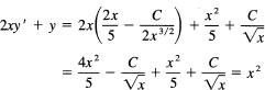
Solve
![]()

Divide through by x2 and you have the exact equation:

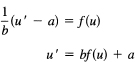
The second form of a second order differential equation we can handle is
y″ = f(y, y′)
with no x term present. We set y′ = ν(velocity if you wish for a mnemonic). We have
![]()
Hence the equation becomes
![]()
which is a first-order equation. We solve this (if we can) and then substitute v = dy/dx to get another first-order equation to solve.
Example 23.9-2
Consider the important equation
y″ + k2y = 0
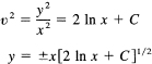
If we use this method (for this equation another method is preferable but it illustrates the method), we are led to
![]()
The variables are separable, and we get finally
ν2 + k2y2 = C2
where it is convenient to make the constant positive. Solving for v, we get (choosing the plus sign for the square root)
Again the variables are separable, and we have
![]()
Integrating, we get
![]()
Take the sine of both sides and solve for y:
![]()
But C / k is a constant, so we may write the solution in the forms
![]()
where C1 and C2 are suitable constants. Had we chosen the minus sign in the square root, things would not have come out differently.
In both of the cases we studied we have reduced the second-order differential equation to a sequence of two first-order differential equations. The importance of these special cases is that they occur frequently in practice.
Solve the following:
1. y″ + ay′ = f(x)
2. y″ + ay′> + by = c
23.10 DIFFERENCE EQUATIONS
Difference equations occur frequently in discrete mathematics, and it is fortunate that the method for solving them closely parallels that for differential equations. We will consider here only the simplest examples.
Consider the first-order linear difference equation
![]()
We do the same as we did for differential equations except that in place of emx we try rn as a trial solution (think of the constant r↔em). The first step is to examine the corresponding homogeneous equation, which is
We try a solution of the form y = rn. The result is
![]()
so r = –a. The general solution of the homogeneous equation is
![]()
The second step is to find one solution of the complete equation. One method is to guess at the solution of the complete equation, and when we find one, any one at all, then the general solution of the complete equation is this particular solution of the complete equation plus the general solution of the homogeneous equation.
Example 23.10-1
Solve
![]()
We naturally try, for the particular solution of the complete equation, an expression of the form
![]()
We get, upon direct substitution,
![]()
from which we get, when we equate the linearly independent terms,
a = 2a + 1, a + b = 2b
whose solutions are
a = –1, b = –1
Hence the particular solution is
![]()
The solution of the homogeneous part is easily found. Assume
![]()
You get
![]()
from which r = 2. The general solution of the complete equation is therefore
![]()
To fit the intitial condition y0 = 1, we have
y0 = 1 = C − 1
from which C = 2, and the final solution is
![]()
Suppose that there are a men and b women and that n chips are passed out to them at random. What is the probability that the total number of chips given to the men is an even number?
We regard this as a problem depending on n. We start with n = 0. The probability that the men have an even number of chips when no chips have yet been offered is
P(0) = 1
We next ask how can the stage n arise? It comes from the stage of n − 1 plus the process of passing out one more chip at random. The n − 1 state is either that the men have an even number of chips, P(n – 1), or that they have an odd number, 1 − P(n − 1). From these we build up the state n by taking these two probabilities and multiplying them by the corresponding probabilities of the nth chip going to a man or a woman. Thus we have the difference equation
![]()
We write this difference equation in the canonical form
![]()
For the moment call b – a)/(b + a) = A. The solution of the homogeneous equation is clearly
CAn
for some constant C. We next need a particular solution of the complete equation. With the right-hand side a constant, we try a constant, say B. We have
![]()
or
Thus th egeneral solution of the difference equation is
![]()
It remains to fit the initial condition P(0) = 1. This gives immediately C = ![]() , and the final solution is
, and the final solution is
![]()
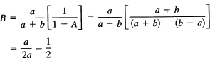
This can be written in a more symmetric form:
![]()
Let us examine this solution for reasonableness. if a = 0, no men, then the solution is
![]()
and certainly the number of chips given at random to the men is an even number (0 is an even number). If a = b, then we have
![]()
and this by symmetry is clearly correct. Finally, if there were no women, b = 0, then
![]()
which alternates between 0 and 1 and again is correct. Thus we have considerable faith in the result found.
1. Suppose that a system can be in one of two states, A or B, and that if it is state A then at the next time interval it has probability pA of going to state B; while if it is in state B it has probability pB of going to state A. Find the probability of being in state A at time n. Check your answer by the three cases you can easily solve: (a) pA = 0, (b) pA = pB, (c) pA = 1, pB = 0.
2. Using complex notation, find the integrals ![]() and the corresponding one with cos x by means of differentiating.
and the corresponding one with cos x by means of differentiating.
23.11 SUMMARY
Differential equations are of fundamental importance in many fields of application of mathematics. Generally, a good deal of knowledge of the field of application is needed to set up the initial differential equations that represent the phenomenon you are interested in. Once set up, it becomes, to a great extent, a matter of solving them using the mathematical tools available.
The method of direction fields tends to be forgotten as trivial and uninteresting, but on several occasions the author has disposed of an important physical problem over lunch by sketching the direction field on the back of a place mat; the sketch showed the nature of the solution, and that was all that was needed to understand the phenomenon.
It is surprising how many practical problems yield to the elementary methods of (1) variables separable and (2) homogeneous equations leading to variables separable, or (3) have an obvious integrating factor. The method of change of variables depends, as it does in integration, on a sudden insight into what might make the problem solvable, and there are few general rules.
Linear differential equations are very important, and their study will be continued in the next chapter.
Finally, we examined linear first-order difference equations. The theory is almost exactly parallel to the theory of linear differential equations. We have not pursued the corresponding analogies between the other methods of solving differential equations and the corresponding difference equations. Generally, integration is replaced by summation, and there are only a few other changes to be considered. You can make an abstraction based on the two special cases, linear differential equations and linear difference equations, to get at the general linear problem, but this lies properly in a course in linear algebra, not in a first course such as this one.