A perfect formulation of a problem is already half its solution.
DAVID HILBERT
All models are wrong, but some are useful.
GEORGE E. P. BOX
In this chapter, we begin the development of the mathematical formalism that answers the four fundamental questions we raised in chapter 1. As noted, none of the mainstream economic theories or the econophysics models or the philosophical frameworks answer these questions.
The goal of our model society, a hybrid utopia called BhuVai, is to empower all citizens to pursue their visions of happiness and to realize those visions in practice. The happiness thus enjoyed by everyone is at the same level. While overall happiness certainly depends on a number of factors such as physical, emotional, and economic health, we restrict ourselves to economic health as our focus is on distributive economic justice. We assume that the citizens in BhuVai are physically and emotionally healthy and therefore are happy as far as these factors are concerned. Our focus is entirely on a person’s work—what it contributes to the society and the happiness derived from it in the form of economic rewards. Since our focus is on distributive economic justice, particularly how income would be distributed in a just manner in our model society, we assume that all other requirements of social justice have already been satisfied in BhuVai.
How, then, would distributive justice be realized in BhuVai? As noted, since different people have different skills and therefore make different contributions to a society, we expect people to be compensated unequally monetarily. So a certain level of income inequality is to be expected. But what is the fairest level of income inequality?
Recall that our hybrid utopia is part Rawlsian and part Nozickian. Following the Nozickian feature, we let this income distribution be achieved through the free-market mechanism. As Nozick argues, whatever income distribution that naturally arises as a result is the fairest outcome according to his libertarian justifications. As noted, the only modification we make to his purely free-market view is to introduce a Rawls-like condition that there is a minimum-wage floor to protect the working poor. Most free-market democracies exhibit these two characteristics. Therefore, the distributive justice question is: In our ideal hybrid free-market environment, what level of inequality should arise naturally? This is the question we address in this chapter and chapter 5.
Note that in our utopia, different levels of incomes do not result in different levels of happiness. For instance, even though an artist may make less than, say, a hedge fund manager, they are both equally happy. This is the key feature of our hybrid utopia (this feature is explored in greater detail in section 8.3 after we have introduced and discussed our framework).
3.1.1 Ideal Versus Real-Life Free Market
To determine this income distribution, we propose the following gedankenexperiment, in which we study a competitive, dynamic free-market environment in BhuVai, comprising a large number of utility-maximizing rational agents as employees and profit-maximizing rational agents as corporations. Let us assume an ideal environment in which the free market is perfectly competitive, transaction costs are negligible, and no externalities are present. There are no biases due to race, gender, religion, etc. We assume that no single agent (or small group of agents), whether an employee or a company, can significantly affect the market dynamics; i.e., there is no rent seeking or market power. In other words, our ideal free market is a level playing field for all its participants. We also assume that neither the companies nor the employees engage in illegal practices such as fraud, collusion, and so on. We also assume moderate scarcity of resources. We do not consider extreme situations in demand or in supply. We do not consider cases wherein there is an extremely high demand, or extremely low demand, for any skills. Similarly, we do not consider cases wherein there is an abundant supply, or an extreme scarcity, of skills. We consider such situations as exceptions rather than the norm in a typical market. We do not consider the effect of taxes as we compare our predictions with real-world pretax income distribution data from Piketty and coworkers in chapter 6. (We plan to address the effect of taxes and transfers in future work, which we discuss in chapter 8.)
In our ideal free market, employees are free to switch jobs and move between companies in search of better utilities. Similarly, companies are free to fire and hire employees to maximize their profits. We also assume that a company needs to retain all its employees in order to survive in this competitive market environment. Thus, a company will take whatever steps necessary, allowed by its constraints, to retain its employees. Similarly, all employees need a salary to survive, and they will do whatever is necessary, allowed by certain norms, to stay employed.
It is important to emphasize that the free market itself, ideal or otherwise, is a human creation and “does not exist in the wilds beyond the reach of civilization” (Reich 2015, 4). As Reich (2015, 3–5) observes, “Few ideas have more profoundly poisoned the minds of more people than the notion of a ‘free market’ existing somewhere in the universe, into which government ‘intrudes.’…A market—any market—requires that the government make and enforce the rules of the game. In most modern democracies, such rules emanate from legislatures, administrative agencies, and courts. Government doesn’t ‘intrude’ on the ‘free market.’ It creates the market.” In our utopia, the government has defined the rules of the game in such a way that the resulting free market behaves ideally.
Real-life free markets are, of course, not ideal. Biases of various kinds are common. As Bebchuk and Fried (2006), Reich (2015), and Stiglitz (2015) argue, rent-seeking behavior by executives has contributed to excessive CEO compensation in recent years, while the deteriorating bargaining power of rank and file employees due to weakened unions has resulted in their diminished share of the income pie. Nevertheless, it is useful to analyze the behavior of an ideal free market as it provides a reference state, identifying what the outcome should be under ideal conditions. We can then compare this result with the outcomes seen in real life, and both assess and correct nonideal behavior through appropriate policy prescriptions. Simply put, we need to understand how an ideal free market behaves before we can analyze all the complexities of a real-life free market.
3.1.2 A Gedankenexperiment in the Ideal Free Market
In this ideal free market, consider a company, named iAvatars Inc., with N employees and a payroll of M, with an average salary of Save = M/N. We assume that there are n categories of employees, ranging from low-level employees to the CEO, contributing in different ways to the company’s overall success and value creation. All the employees contribute to the company’s overall success in their own ways. The cleaning crew keeps the premises neat, the secretarial staff helps with organization and communication, engineers develop products and services, marketing and sales personnel bring new orders, accounting and finance personnel mind the books, management focuses on a winning corporate strategy and execution, and so on. How do we value all employees’ contributions and reward them fairly?
All employees in category i contribute value Vi, i ∈ {1, 2,…, n} such that V1 < V2 < · · · < Vn. Let the corresponding value at Save be Vave, occurring at category s. Since employees are contributing unequally, they need to be compensated differently, commensurate with their relative contributions to the overall value created by the company. Instead, iAvatars has an egalitarian policy that all employees are equal, and therefore it pays all of them the same salary Save irrespective of their contributions. The salary of the CEO is the same as that of a janitor. This salary distribution is a sharp vertical line at Save, as seen in figure 3.1(a), which is the Kronecker delta function.
While this may seem fair in a social or moral justice sense (this distribution has a Gini coefficient of 0), clearly it is not in an economic sense. If iAvatars were the only company in the economic system, or if it were completely isolated from other companies in the economic environment, then the employees would be forced to continue to work under these conditions as there would be no other choice.
However, in an ideal free-market system there are choices. Therefore, employees who contribute more than the average, i.e., those in value categories Vi such that Vi > Vave (e.g., senior engineers, vice presidents, CEO), who feel that their contributions are not fairly valued and compensated by iAvatars will therefore be motivated to leave for other companies where they are offered higher salaries. Hence, to survive, iAvatars will be forced to match the salaries offered by others to retain these employees, thereby forcing the distribution to spread to the right of Save, as seen in figure 3.1(b).
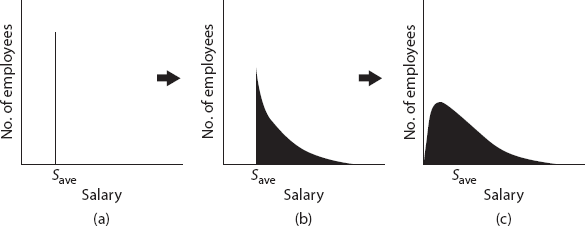
At the same time, the generous compensation paid to all employees in categories Vi such that Vi < Vave will motivate candidates with the relevant skill sets (e.g., low-level administration, sales, and marketing staff) from other companies to compete for these higher-paying positions in iAvatars. This competition will eventually drive the compensation down for these overpaid employees, forcing the distribution to spread to the left of Save, as seen in figure 3.1(c). Eventually, we will have a distribution that is not a delta function, but a broader one where different employees earn different salaries depending on the values of their contributions as determined by the free-market mechanism. The funds for the higher salaries now paid to the formerly underpaid employees (i.e., those who satisfy Vi > Vave) come out of the savings resulting from the reduced salaries of the formerly overpaid group (i.e., those who satisfy Vi < Vave), thereby conserving the total salary budget M.
Thus, we see that concerns about fairness in pay cause the natural emergence of a more equitable salary distribution in a free-market environment through its self-organizing, adaptive, and evolutionary dynamics. The point of this analysis is not to model the exact details of the free-market dynamics, but to show that the notion of fairness plays a central role in driving the emergence and spread of the salary (in general, utility) distribution through the free-market mechanism.
Even though an individual employee cares only about her utility and no one else’s, the collective actions of all the employees, combined with the profit-maximizing survival actions of all the companies, in an ideal competitive free-market environment of supply and demand for talent under resource constraints, lead toward a more fair allocation of pay, guided by Adam Smith’s “invisible hand” of self-organization. This is the invisible hand process that Nozick refers to in his libertarian proposal. So, instead of state-imposed maximin allocation aimed at achieving distributive justice, as Rawls recommends, the free-market dynamics determines the level of income inequality naturally. In chapter 5 we will prove that this is the fairest outcome not only in the Nozickian sense but also in the system-theoretic sense.
We have used salary as a proxy for utility (i.e., happiness derived from work) in this example to motivate the problem (we use the term utility to stand for happiness, welfare, or well-being in the rest of this book). In general, utility is a complicated aggregate that depends on a host of factors, some measurable, others not. Obviously, pay (i.e., total compensation including base salary, bonus, options, etc.) is an important component of utility, generally the dominant one. Other components include the quantity and quality of the effort, title and peer recognition, competition and job security, career and personal growth opportunities, retirement and health benefits, company culture and work environment, job location, and so on, not necessarily in that order.
Given this free-market dynamics scenario, three important questions arise: (1) Will the self-organizing free-market dynamics lead to an equilibrium salary distribution, or will the distribution continually evolve without ever settling down? (2) If there exists an equilibrium salary distribution, what is it? (3) Is this distribution fair? These are essentially the same as the first two questions from chapter 1, refined by our gedankenexperiment.
Our knowledge of the free-market dynamics, as well as of distributive justice, is incomplete, in a fundamental way, without an answer to these critical questions. This requires a theoretical understanding of the free-market dynamics, at a reasonable level of depth, particularly from the bottom up, agents-based, microeconomic perspective as described above. Given the obvious complexity of real-life free-market dynamics, it is unrealistic to expect to develop a theory, and the associated models, that will address all the details and nuances. Therefore, our goal is to develop an analytical framework that identifies the key concepts and general principles, that models free-market dynamics under ideal conditions, and that answers these central questions. We develop such a framework in the following sections.
We address these questions by developing a microeconomic framework based on potential game theory (There is a brief introduction to potential game theory below.) Continuing with the scenario described above, we assume that all employee agents get “dissatisfied,” now and then, in their current positions. After working in the same position for a while, every employee feels that she has learned all that could be learned and so it is time for her to move up in her career. Every employee feels, sooner or later, that she could be and should be doing better, given her talents and experience, in her company or elsewhere. As a result, employees are on the lookout for job opportunities to improve their utilities. That is, these utility-maximizing, fairness-seeking, teleological agents become restless, now and then, itching to move to a better position.
Let us now examine the basic question of why people seek employment. At the most fundamental level, survival is to be able to pay bills now so that they can make a living, with the hope that the current job will lead to a better future. One hopes that the present job will lead to a better one, acquired based on the experience from the current job, and to a series of better jobs in the future, hence to a better life. This opportunity for a better future, with the expectation of upward mobility, is valuable to most, if not all, of us. This is the utility of having a fair shot at better future prospects. We are, of course, prepared to put in the requisite effort to earn such a life. This effort includes not only the effort we would put into our present jobs but also the effort (and time and money) we invested in the past to acquire the requisite education, skills, and experience. Thus, the utility derived from a job is made up of two components: the immediate benefits of making a living (i.e., “present utility”) and the prospects of a better future life (i.e., “future utility”).
Hence, we propose that the overall or effective utility from a job is determined by three dominant elements: (1) utility from salary, (2) disutility from effort, and (3) utility from a fair opportunity for recognition and career advancement. By effort, we do not mean just the physical effort alone, as we discuss later, even though that is a part of it. This overall utility is the microeconomic foundation on which we build our theory to predict and explain the emergent macroeconomic consequences in pay distribution in an ideal free-market environment.
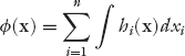
Thus, the effective utility for an agent is given by
where hi is the effective utility (i.e., happiness from work) of an employee earning a salary Si by expending an effort Ei, while competing with Ni −1 other agents in the same job category i for a fair recognition of one’s contributions. Here u(·) is the utility derived from salary, v(·) is the disutility from effort, and w(·) is the utility from a fair opportunity for a better future. Every agent tries to maximize effective utility by picking an appropriate job category i.
3.2.1 Utility of a Fair Opportunity for a Better Future
The first two elements are rather straightforward to appreciate, but the third requires further discussion. The first two elements model the tendency of an employee to maximize one’s utility from salary while minimizing the effort put into receiving it.
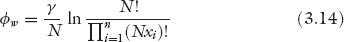
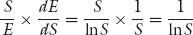
As for the third element, consider the following scenario. A group of freshly minted law school graduates (totaling Ni) have just been hired by a prestigious law firm as associates. They have been told that one of them will be promoted to partner in eight years depending on their performances. Let us say that the partnership is worth $Q. So any associate’s chance of winning the coveted partnership goes as 1/Ni, where Ni is the number of associates in her peer group i, her local competition. Therefore, her expected value for the award is Q/Ni, and the utility derived from it goes as ln(Q/Ni) because of diminishing marginal utility. Therefore, the utility derived from a fair opportunity for recognition and career advancement in a competitive environment is1

where γ is a parameter. This equation models the effect of competitive interaction among agents. In considering the society at large, this equation captures the notion that in a fair society, an appropriately qualified agent with the necessary education, experience, and skills should have a fair shot at growth opportunities irrespective of her race, color, gender, and other such factors; i.e., it is a fair competitive environment. This is the utility derived from equality of access for a better life, for upward mobility. This is the utility of having a fair shot at a better future. Category i would correspond to her qualification category in the society. The other agents in that category are the ones she will be competing with for these growth opportunities. We note that this mathematical expression captures what Rawls mentioned qualitatively in the first part of his second principle, fair equality of opportunity. We weren’t particularly looking to model this Rawlsian requirement, but, as we see, it emerges naturally in our formulation as an integral feature.
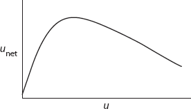
3.2.2 Modeling the Disutility of a Job: Net Utility’s Inverted U-profile
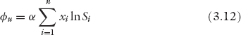
For the utility derived from salary, we employ the commonly used logarithmic utility function
where α is a parameter. As for the second element, every job has a certain disutility associated with it. This disutility depends on a host of factors such as the investment in education needed to qualify oneself for the job, the experience to be acquired, working hours and schedule, quality of work, work environment, company culture, relocation anxieties, etc., which are often difficult, if not impossible, to quantify accurately in real life. While there is considerable prior work on modeling the disutility of effort when a metric for effort is available (Fehr et al. 1998; Laffont and Tirole 1993; Cadenillas et al. 2002; Böhringer and Löschel 2013; Dossani 2002), there isn’t much when such a metric is absent.
In the absence of such a metric, typically one compensates for these different uncertain components of the disutility of a new job by negotiating a salary package that would make it worth the undertaking. Thus, in practice, one intuitively uses salary as a proxy to impute and estimate the “cost” of the job, thereby estimating the remuneration required to compensate for the disutility of effort. Note, again, that by effort we mean not just the hours put into performing the job, but all the prior investment in education and experience to qualify for the position as well as the other adjustments and sacrifices to be made in the new position. There is empirical evidence that supports this line of reasoning in the work of Stratton (2001) and Ahituv and Lerman (2007), who have demonstrated that effort correlates with ln(S).
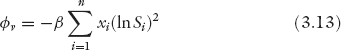
Combining this with the commonly used quadratic disutility from effort (Laffont and Tirole 1993; Cadenillas et al. 2002; Böhringer and Löschel 2013; Dossani 2002; Holmstrom and Milgrom 1991; Nalebuff and Stiglitz 1983; Laffont and Tirole 1988, 1987; Zabojnik 1996), we propose the following form for the second element:
where β is a parameter. Our formulation is also consistent with the conditions imposed on effort E as a function of salary, E(S). According to Katz (1986) and Akerlof and Yellen (1986), E(S) should satisfy the following conditions:
Our effort function E(S) = lnS satisfies all three conditions:
1. 
2. E(0) = −∞ < 0
3.  is decreasing.
There is also another simpler, more intuitive way to arrive at equation (3.4). Combine u and v to compute
which is the net utility (i.e., net benefit or gain) derived from a job after accounting for its cost. Typically, net utility will increase as u increases (e.g., because of salary increase). However, generally, after a point, the cost has increased so much—due to personal sacrifices such as working overtime, missing quality time with family, giving up on hobbies, job stress resulting in poor mental and physical health, etc.—that unet begins to decrease after reaching a maximum (see figure 3.2).
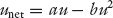
The simplest model of this commonly occurring inverted-U profile is a quadratic function, as in
Since u ∼ ln(S), we get equation (3.4). We believe this is the simplest expression that captures this typical, widely observed behavior of net utility—increasing first and then decreasing. Therefore, our formulation for effort is a reasonable one supported by empirical evidence as well as by intuitive and theoretical expectations.
Note that most things in life in which the benefit gained has a cost associated with it have this inverted-U curve trend seen in figure 3.2. Consider, e.g., taking some medicine to cure an ailment. If you are suffering from a severe headache, taking one Tylenol might make you feel a little better, but taking two might help more. This doesn’t mean that taking ten would help a lot more! It could actually make you sicker, triggering a whole set of other, more serious problems such as kidney disease and bleeding in the digestive tract. As the dosage increases beyond a critical point, the benefit begins to go down, sometimes dramatically. This is so because the cost of the treatment (in the form of negative side effects) begins to exceed the benefit.
Another such example can be seen in exercising. If running an hour per day is good for you, running ten hours per day, every day, is not necessarily great for you (i.e., for most people, excluding gifted long-distance athletes), because of the serious wear and tear on various body parts. The hedge fund titans who went bust in the subprime crisis learned this annoying little fact the hard way when they relied on excessive leverage to generate their outsized returns. Leverage of 2 to 3 (i.e., taking moderate risk) can be helpful to juice up the returns ordinarily, but when it is over 30, the downside is just disastrous. There are many such examples from all walks of life. In summary, more isn’t always better, because most benefits usually have costs associated with them. Our utility function captures and models this essential and near-universal trait in most things in life.
3.2.3 Effective Utility Enjoyed from a Job
Combining all three, we have
where α, β, γ > 0.
In general, α, β, and γ, which model the relative importance an agent assigns to these three elements, can vary from agent to agent. However, we first examine the ideal situation in which all agents have the same preferences and hence treat these as constant parameters. (In sections 5.10 and 6.5, we relax this requirement and consider other cases. We also discuss what these parameters imply in greater detail in section 8.4.) As noted, presumably there are other expressions one could use to model these three elements, but the choices we made have interesting properties, revealing important insights and connections, as we shall see shortly.
To move to a job with better utility, an agent needs job offers. So the employee agents constantly gather information and scout the market, and their own companies, for job openings commensurate with their skill sets, experiences, and career and personal goals. Similarly, the company agents (e.g., through the human resources department) also conduct similar searches, looking for opportunities to fire and hire employees so that their profits may be improved.
At any given time, an employee agent is faced with one of five job options: (1) no new job offer is available, (2) the new offer has the same utility as the current one, (3) the new offer has less utility than the current one, (4) the new offer has greater utility, or (5) the employee agent is let go from the current job (i.e., zero utility). The agent’s best strategies for the five options are as follows: for (1), (2) and (3), the agent stays put in the current position at the current utility; for (4) the agent accepts the new offer; and for (5) the agent leaves the company and looks for a new position. Each agent’s strategy is independent of what other agents are doing.
We are now ready to answer these questions: (1) Is there an equilibrium salary distribution? (2) If yes, what is it?
We answer these questions by using two different, but related, approaches. The first approach, which we call the bottom-up perspective, uses concepts and techniques from game theory. The second approach, which we call the top-down perspective, uses concepts and techniques from statistical mechanics and information theory. We develop the former in this chapter and the latter in chapter 5.
3.3.1 Game Theory: Players, Strategies, and Equilibrium
Before we jump into the technical details, let us start with an informal background to game-theoretic concepts for nonexperts.2 The problem from section 3.1 is the following: Given a set of strategically interacting rational agents (called players), where each agent is trying to decide and execute the best possible course of action that maximizes the agent’s outcome (called payoff) in light of similar strategies executed by the other agents, we are interested in predicting what strategies will be executed and what outcomes are likely. In other words, what are the possible outcomes of the strategic behaviors of the employees and the company in our thought experiment?
Game theory is a mathematical framework for answering this question by systematically analyzing and predicting the decision-making strategies, the dynamic behavior, and the likely payoffs of players, using models of conflict and cooperation. Just as probability theory originated from the study of pure gambling without strategic interaction, game theory originated from the formal study of strategic games, such as chess or Le Her, a card game. While some game-theoretic ideas could be traced as far back as the Babylonian Talmud (Walker 2012), most people generally credit the groundbreaking book The Theory of Games and Economic Behavior, by John von Neumann and Oskar Morgenstern, published in 1944, as the origin of the mathematical study of game theory. Great progress was made in the subsequent two decades, which is when famous game theory problems such as the prisoner’s dilemma3 were invented. This was also the period when John Nash made his seminal contribution (Nash 1950, 1951), which is central to the question we raised above.
Drawing the distinction between cooperative games, in which binding agreements can be made, and noncooperative games, where they are not feasible, Nash proved the existence of a strategic equilibrium, now called the Nash equilibrium, for noncooperative games. In a Nash equilibrium outcome, no player can unilaterally move to improve her own payoff. In other words, players have no incentive to change their actions, since their current strategy is the best they can do, given the actions of the other players.
The concept of an equilibrium, whose existence or nonexistence can be predicted through a systematic analysis of the game, is one of the most fundamental results in game theory with far-reaching implications in economics, sociology, political science, biology, and engineering. All these disciplines are riddled with situations in which one is interested determining the eventual outcome of a set of players making strategic decisions—one wants to know whether this ultimate outcome is an equilibrium state. This is exactly the same question we have in our problem above.
Interestingly, it is the same question that arises when one is dealing with a large number of entities that are interacting not strategically but randomly, such as molecules of a gas enclosed in a container. We want to know the equilibrium state for the gas and what criterion determines it. This problem is solved by using a mathematical framework called statistical mechanics, which is founded on probability theory. As noted, probability theory originated from the study of games of chance, whereas game theory originated from games of strategy. Since both mathematical frameworks define and determine an equilibrium state, it is natural to ask whether there is any connection between the two approaches. As it turns out, there is a deep, beautiful, and hitherto unknown connection with surprising and useful insights. We explore this in chapter 5.
Nash was recognized for his pioneering contributions with the Nobel Prize for Economic Sciences (officially, the Sveriges Riksbank Prize in Economic Sciences in Memory of Alfred Nobel), in 1994, which he shared with fellow game theorists John C. Harsanyi and Reinhard Selten. This was the first Nobel awarded for work in game theory. Some readers might recall that the life and achievements of John Nash were celebrated in the Hollywood movie A Beautiful Mind.
3.3.2 Population Games and the Potential Function
Among the many classes of games, there is a class called population games that is particularly relevant to the situation described in our gedankenexperiment.4 This class studies games with a large number of players, as in our example. It provides an analytical framework for studying the strategic interactions of a population of agents with the following properties, as described by Sandholm (2010): (1) The number of agents is large. (2) Individual agents play a small role—any one agent’s behavior has only a small effect on other agents’ payoffs. (3) Agents interact anonymously—each agent’s payoffs depend on only the opponents’ behavior through the distribution of their choices. (4) The number of roles is finite—each agent is a member of one of a finite number of populations. (5) Payoffs are continuous—this property ensures that very small changes in aggregate behavior do not lead to large changes in payoffs. We note that these properties more than adequately account for the features of our game played in the gedankenexperiment.
In games like prisoner’s dilemma, with a small number of players, the typical game-theoretic analysis proceeds by systematically evaluating all the options every player has, determining the payoffs, writing the payoff matrix, identifying the best responses of all players, and identifying the dominant strategies (if present) for everyone, and then finally reasoning whether there exists a Nash equilibrium (or multiple equilibria). However, for population games, given the large number of players, this procedure is not feasible for several reasons. For instance, a player may not know of all the strategies others are executing (or could execute), and their payoffs, in order for her to determine her best response.
Fortunately, as it turns out, for some population games one can identify a single scalar-valued global function, called a potential, that captures the necessary information about payoffs. The gradient of the potential is the payoff or the utility. Such games are called potential games. The origins of potential game theory can be traced to the concept of a congestion game proposed by Rosenthal (1973). Rosenthal proved that any congestion game is a potential game, and Monderer and Shapley later proved the converse (Monderer and Shapley 1996)—for any potential game, there exists a congestion game with the same potential function.
A SIMPLE EXAMPLE: TRAFFIC CONGESTION A congestion game commonly arises in analyzing problems such as congestion in traffic networks. We illustrate this with a simple example. Consider driving from home to work, where you have two route choices. Route R1 is wider with a width of a1, and route R2 is narrower with a width of a2 (that is, a1 > a2). Assume that the travel time t, from home to work, goes inversely as the width; i.e., the wider route tends to be faster than the narrower route. Let us further assume that both a1 and a2 have some lower and upper bounds. The bounds don’t really matter for the reasoning below; they are only there to avoid the unrealistic outcomes such as t1 = 0 or t2 = 0 when a1 = ∞ or a2 = ∞. Let us also assume that t increases linearly with the amount of traffic on the route, i.e., the congestion. In other words, t increases as the number of cars N on that route increases.
Initially, since R1 is wider and hence faster, many drivers will choose that as their best response. This would increase its traffic load, i.e., congestion, which in turn increases the travel time in that route. This will discourage other drivers from switching to it and will encourage them to choose R2 as their best response now. In this manner, drivers will self-organize and distribute themselves between the two alternatives, so that ultimately the travel time from home to work is the same in both routes, i.e., the equilibrium state. At equilibrium, there is no incentive for any driver to switch from his current route to the other, as the travel time is the same in both.
This is what we would expect to happen intuitively. Let us see whether the math bears this out. Given the problem description above, we have the following relations:
where t1 and t2 are travel times on routes R1 and R2, respectively. Variables N1 and N2 are the number of cars on the two routes, x1 and x2 are fractional allocations of cars, and N is the total number of cars on both routes.
The goal for every driver, of course, is to minimize her travel time t from home to work. By minimizing the travel time, every driver is maximizing her utility or welfare. The travel time is the cost of the commute, and negative cost is the utility or the benefit. Therefore, we write the utility h for the two routes as
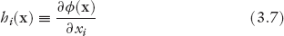
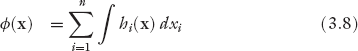
As noted, in potential games, a player’s payoff or utility is the gradient of potential ϕ(x), i.e., (3.7)
where xi = Ni/N and x is the population vector. Therefore, by integration [we replace the partial derivative with the total derivative because hi(x) can be reduced to hi(xi)], we have
The potential ϕ(x) is therefore
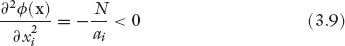
We can show that ϕ(x) is strictly concave:
Therefore, a unique Nash equilibrium for this game exists, where ϕ(x) is maximized, per the well-known theorem in potential games (Sandholm 2010, 60).
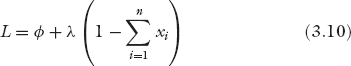
To determine the maximum potential, we use the method of Lagrange multipliers with L as the Lagrangian and λ as the Lagrange multiplier for the constraint  :
:
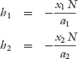
Solving ∂L/∂xi = 0, we obtain the following result at equilibrium:
We note that at equilibrium, the condition that h1 = h2 = λ, which is the same as t1 = t2, is exactly what was expected intuitively above—the travel times are the same in both routes. Furthermore, if both routes were equally wide, i.e., a1 = a2, then x1 = x2. So both routes will have the same number of cars as well, which is again what we would expect intuitively. So the math validates our intuition.
This is a useful result to explore further. You are told initially that there are two routes from home to work and that both are identical in all respects. You are also told there is a combined total of N cars traveling in both routes. Then you are asked how the cars are distributed between the two routes, i.e., how many cars are traveling in route R1 versus R2. Since both routes are identical, there is no reason to prefer one over the other, and hence you would answer that the cars are distributed evenly. This would be the fairest distribution of cars between the two routes. There is no reason to assign more cars to one route and fewer cars to the other route. Clearly that wouldn’t be fair.
Now, consider another scenario. You are told R1 is twice as wide as R2, or a1 = 2a2. You know this means R1 is twice as fast as R2, at least initially. That means it will attract more cars, which, of course, will slow it down. So, you’d reason that at equilibrium R1 will have twice as many cars as R2. This is the fairest distribution now. Keep these results in mind for now, particularly the relationship among a distribution, its fairness, and the problem constraints, for this connection is revisited in chapter 5.
This example is meant only as a simple illustration of best response dynamics in potential games, to give a nonexpert reader a quick introduction to the nature of the analysis. Interested readers are encouraged to see Easley and Kleinberg (2010) or Sandholm (2010) for a more thorough treatment of congestion games.
With this quick introduction to potential games, we now turn our attention back to the gedankenexperiment to answer this question: Is there an equilibrium income distribution?
Since our problem is a population game with features of a congestion game, we again use the potential game framework to address this question. Recall that an employee’s utility is the gradient of potential ϕ(x), or
where xi = Ni/N and x is the population vector. Therefore, by integration [again, we replace the partial derivative with the total derivative because hi(x) can be reduced to hi(xi), expressed in equations (3.1) through (3.4)]
We observe that our game is a potential game with the potential function
where
We can show that ϕ(x) is strictly concave:
Therefore, as before, a unique Nash equilibrium for this game exists, where ϕ(x) is maximized.
Thus, the self-organizing free market dynamics, in which employees switch jobs and companies switch employees in search of better utilities or profits, ultimately reaches an equilibrium state, with an equilibrium income distribution. This happens when the potential ϕ(x) is maximized.
This immediately raises two questions: (1) What is the equilibrium income distribution? (2) What is the economic meaning of the potential function?
The first question is, in fact, the first question in the original set of four questions we raised in chapter 1. The second question here is new, but it turns out to be crucial also. We discuss and answer both questions in chapter 5.
Readers familiar with statistical mechanics will recognize the potential component ϕw as entropy (except for the missing Boltzmann constant kB). This identification suggests that maximizing the payoff potential in game-theoretic equilibrium would correspond to maximizing entropy in statistical mechanical equilibrium, thereby revealing a deep and useful connection between these seemingly different conceptual frameworks. This connection suggests that one may view the statistical mechanics approach to molecular dynamics, also called statistical thermodynamics, from a potential game perspective. In this approach, one may view the molecules as restless agents in a game (let’s call it the thermodynamic game), continually jumping from one energy state to another through intermolecular collisions. However, unlike employees who are continually driven to switch jobs in search of better utilities they desire, molecules are not teleological, i.e., not goal-driven, in their constant search. As prisoners of Newton’s laws and conservation principles, constantly subjected to intermolecular collisions, their search and dynamical evolution are the result of thermal agitation.
We explore this connection in the next two chapters. In chapter 4, we first provide a simple, intuitive introduction to statistical thermodynamics and its key concepts, particularly entropy and statistical equilibrium. In chapter 5, we utilize this connection to derive formal and useful results regarding the income distribution in BhuVai.