What is involved in the engineering of a wireless system? When your mobile phone rings, a set of actions has already been put in motion to allow you to stay effortlessly connected to a vast communication network not dreamed of by your parents. Several disciplines, theoretical studies, technologies, and engineering developments have converged to create this wonder, and it starts with the invisible radio frequency (RF) link connecting your mobile phone to one of the ubiquitous base station towers around your town. To begin our study of wireless systems engineering, we first investigate RF links. The engineering of these connections will introduce the process of systems engineering that will take us through most of the physical system design.
Two fundamental and interrelated design considerations for a wireless communication system are
Note that capacity may be expressed in a number of ways. It may be expressed as the number of simultaneous two-way conversations that can take place, the average data rate available to a user, the average throughput for data aggregated over all users, or in many other ways, each related to the nature of the information being communicated. It should become apparent in later discussions that area and capacity criteria are interdependent from both technical and economic viewpoints. For wireless systems, coverage area and capacity are intimately related to the attributes of the RF link (or, in cellular telephone terminology, the "air interface"), and thus we begin our study with an overview of this type of link.
Most people have experienced the degradation and eventual loss of a favorite broadcast radio station as they drive out of the station's coverage area. This common experience clearly demonstrates that there are practical limits to the distance over which a signal can be reliably communicated. Intuition suggests that reliable reception depends on how strong a signal is at a receiver and that the strength of a signal decreases with distance. Reception also depends on the strength of the desired signal relative to competing phenomena such as noise and interference that might also be present at a receiver input. In fact, the robustness of a wireless system design strongly depends on the designers' abilities to ensure an adequate ratio of signal to noise and interference over the entire coverage area. A successful design relies on the validity of the predictions and assumptions systems engineers make about how a signal propagates, the characteristics of the signal path, and the nature of the noise and interference that will be encountered.
Among the many environmental factors systems engineers must consider are how a signal varies with distance from a transmitter in the specific application environment, and the minimum signal level required for reliable communications. Consideration of these factors is a logical starting point for a system design. Therefore, to prepare for a meaningful discussion of system design, we must develop some understanding of how signals propagate and the environmental factors that influence them as they traverse a path between a transmitter and a receiver.
In this chapter we investigate how an RF signal varies with distance from a transmitter under ideal conditions and how the RF energy is processed in the early stages of the receiver. Specifically, we first introduce the concept of path loss or free-space loss, and we develop a simple model to predict the increase in path loss with propagation distance. Afterward, we investigate thermal noise in a receiver, which leads to the primary descriptor of signal quality in a receiver—the signal-to-noise ratio or SNR. This allows us to quantitatively describe the minimum signal level required for reliable communications. We end our discussion with examples of how quantitative analysis and design are accomplished for a basic RF link. In the next chapter we will discuss path loss in a real-world environment and describe other channel phenomena that may limit a receiver's ability to reliably detect a signal or corrupt the information carried by an RF signal regardless of the signal level.
Electromagnetic theory, encapsulated in Maxwell's equations, provides a robust mathematical model of how time-varying electromagnetic fields behave. Although we won't deal directly with Maxwell's equations, our discussions are based on the behavior they predict. We begin by pointing out that electromagnetic waves propagate in free space, a perfect vacuum, at the speed of light c. The physical length of one cycle of a propagating wave, the wavelength λ, is inversely proportional to the frequency f of the wave, such that
For example, visible light is an electromagnetic wave with a frequency of approximately 600 THz (1 THz = 1012 Hz), with a corresponding wavelength of 500 nm. Electric power in the United States operates at 60 Hz, and radiating waves would have a wavelength of 5000 km! A typical wireless phone operating at 1.8 GHz emits a wavelength of 0.17 m. Obviously, the range of wavelengths and frequencies commonly dealt with in electromagnetic science and engineering is quite vast.
In earlier studies you learned how to use Kirchhoff's laws to analyze the effects of arbitrary configurations of circuit elements on time-varying signals. A fundamental assumption underlying Kirchhoff's laws is that the elements and their interconnections are very small relative to the wavelengths of the signals, so that the physical dimensions of a circuit are not important to consider. For this case, Maxwell's equations reduce to the familiar rules governing the relationships among voltage, current, and impedance. This case, to which Kirchhoff's laws apply, is commonly called lumped-element analysis. When the circuit elements and their interconnections are comparable in physical size to the signal wavelengths, however, distributed-element or transmission-line analysis must be employed. In such cases the position and size of the lumped elements are important, as are the lengths of the interconnecting wires. Interconnecting wires that are not small compared with a wavelength may in fact be modeled as possessing inductance, capacitance, and conductance on a per-length (distance) basis. This model allows the interconnections to be treated as a network of passive elements, fully possessing the properties of a passive circuit. It also explains the fact that any signal will be changed or distorted from its original form as it propagates through the interconnection in much the same way as any low-frequency signal is changed as it propagates through a lumped-element circuit such as a filter. Furthermore, when a circuit is comparable in size to a signal wavelength, some of the electromagnetic energy in the signal will radiate into the surroundings unless some special precautions are employed. When such radiation is unintentional, it may cause interference to nearby devices. In some cases, however, such radiation may be a desired effect.
An antenna is a device specifically designed to enhance the radiation phenomenon. A transmitting antenna is a device or transducer that is designed to efficiently transform a signal incident on its circuit terminals into an electromagnetic wave that propagates into the surrounding environment. Similarly, a receiving antenna captures an electromagnetic wave incident upon it and transforms the wave into a voltage or current signal at its circuit terminals. Maxwell's equations suggest that for an antenna to radiate efficiently its dimensions must be comparable to a signal wavelength (usually 0.1 λ or greater). For example, a 1 MHz signal has a wavelength of 300 m (almost 1000 feet). Thus an antenna with dimensions appropriate for efficient radiation at that frequency would be impractical for many wireless applications. In contrast, a 1 GHz signal has a wavelength of 0.1 m (less than 1 foot). This leads to a practical constraint on any personal communication system; that is, it must operate in a frequency band high enough to allow the efficient transmission and reception of electromagnetic waves using antennas of manageable size.
An electromagnetic wave of a specific frequency provides the link or channel between transmitting and receiving antennas located at the endpoints, over which information will be conveyed. This electromagnetic wave is called a carrier, and as discussed in Chapter 1, information is conveyed by modulating the carrier using a signal that represents the information.
Development of the range equation is greatly facilitated by considering how a signal propagates in free space. By "free space" we mean a perfect vacuum with the closest object being infinitely far away. This ensures that the signal is not affected by resistive losses of the medium or objects that might otherwise reflect, refract, diffract, or absorb the signal. Although describing the propagation environment as free space may not be realistic, it does provide a useful model for understanding the fundamental properties of a radiated signal.
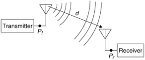
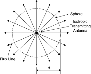
To begin, consider a transmitting antenna with power level Pt at its input terminals and a receiving antenna located at an arbitrary distance d from the transmitting antenna as shown in Figure 2.1. In keeping with our free-space simplification we consider that the transmitter and receiver have a negligible physical extent and, therefore, do not influence the propagating wave. We further assume that the transmitting antenna radiates power uniformly in all directions. Such an antenna is known as an isotropic antenna. (Note that an isotropic antenna is an idealization and is not physically realizable. Neither is an antenna that radiates energy only in a single direction.)
Figure 2.1. Free-Space Link Geometry
Imagine flux lines emanating from the transmitting antenna, where every flux line represents some fraction of the transmitted power Pt. Since radiation is uniform in all directions, the flux lines must be uniformly distributed around the transmitting antenna, as is suggested by Figure 2.2. If we surround the transmitting antenna by a sphere of arbitrary radius d, the number of flux lines per unit area crossing the surface of the sphere must be uniform everywhere on the surface. Thus, the power density p measured at any point on the surface of the sphere must also be uniform and constant. Assuming no loss of power due to absorption by the propagation medium, conservation of energy requires that the total of all the power crossing the surface of the sphere must equal Pt, the power being radiated by the transmitter. This total power must be the same for all concentric spheres regardless of radius, although the power density becomes smaller as the radius of the sphere becomes larger. We can write the power density on the surface of a sphere of radius d as
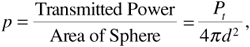
Figure 2.2. Isotropic Radiation Showing Surface of Constant Power Density and Flux Lines
where p is measured in watts per square meter.
Example
Suppose the isotropic radiator of Figure 2.2 is emitting a total radiated power of 1 W. Compare the power densities at ranges of 1, 10, and 100 km.
Solution
The calculation is a straightforward application of Equation (2.2), giving the results p = 80 x 10-9 W/m2, 800 x 10-12 W/m2, and 8 x 10-12 W/m2, respectively. There are two things to note from these results. First, the power density numbers are very small. Second, the power density falls off as 1/d2, as expected from Equation (2.2). Obviously transmission range is a very important factor in the design of any communication link.
A receiving antenna located in the path of an electromagnetic wave captures some of its power and delivers it to a load at its output terminals. The amount of power an antenna captures and delivers to its output terminals depends on its effective aperture (area) Ae, a parameter related to its physical area, its specific structure, and other parameters. Given this characterization of the antenna, the power intercepted by the receiver antenna may be written as

where the r subscript on the antenna aperture term refers to the receiving antenna.
At this point we understand that received power varies inversely as the square of the distance between the transmitter and receiver. Our formulation assumes an isotropic transmitter antenna, an idealization that models transmitted power as being radiated equally in all directions. For most practical applications, however, the position of a receiver relative to a transmitter is much more constrained, and we seek to direct as much of the power as possible toward the intended receiver. We will learn about "directive" antennas in the next section.
Although the design of antennas is a subject for experts, a systems engineer must be able to express the characteristics of antennas needed for specific applications in terms that are meaningful to an antenna designer. Therefore, we discuss some of the concepts, terms, and parameters by which antennas can be described before continuing with our development of the range equation.
A rock dropped into a still pond will create ripples that appear as concentric circles propagating radially outward from the point where the rock strikes the water. Well-formed ripples appear at some distance from the point of impact; however, the motion of the water is not so well defined at the point of impact or its immediately surrounding area.
A physically realizable antenna launches both electric and magnetic fields. At a distance sufficiently far from the antenna we can observe these fields propagating in a radial direction from the antenna in much the same fashion as the ripples on the surface of the pond. The region of well-defined radially propagating "ripples" is known as the far-field radiation region, or the Fraunhofer region. It is the region of interest for most (if not all) communication applications. Much nearer to the antenna there are capacitive and inductive "near" fields that vary greatly from point to point and rapidly become negligible with distance from the antenna. A good approximation is that the far field begins at a distance from the antenna of

where l is the antenna's largest physical dimension.[1] Often in communication applications, the antenna's physical dimensions, though greater than λ/10, are less than a wavelength, so that the far field begins at a distance less than twice the largest dimension of the antenna. For cellular telephone applications, the far field begins a few centimeters away from the handset.
A polar plot of the far-field power density as a function of angle referenced to some axis of the antenna structure is known as a power pattern. The peak or lobe in the desired direction is called the main lobe or main beam. The remainder of the power (i.e., the power outside the main beam) is radiated in lobes called side lobes. "Directive" antennas can be designed that radiate most of the antenna input power in a given direction.
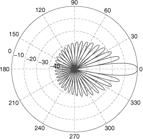
Figure 2.3 illustrates the beam pattern of a directive antenna with a conical beam. The antenna is located at the left of the figure from which the several lobes of the pattern emanate. The plot represents the far-field power density measured at an arbitrary constant distance d from the antenna, where d > dfar field. The shape of the beam represents the power density as a function of angle, usually referenced to the peak of the main beam or lobe. For the antenna represented in the figure, most of the power is radiated within a small solid angle directed to the right in the plot. In general, a convenient coordinate system is chosen in which to describe the power pattern. For example, one might plot the power density versus the spherical coordinates θ and Φ for an antenna oriented along one of the coordinate axes as shown in Figure 2.4. For each angular position (θ, Φ), the radius of the plot represents the value of power density measured at distance d. Since d is arbitrary, the graph is usually normalized by expressing the power density as a ratio in decibels relative to the power density value at the peak of the pattern. Alternatively, the normalization factor can be the power density produced at distance d by an isotropic antenna, see Equation (2.2). When an isotropic antenna is used to provide the reference power density, the units of power density are dBi, where the i stands for "isotropic reference." Figure 2.5 shows an antenna power pattern plotted versus one coordinate angle θ with the other coordinate angle Φ held constant. This kind of plot is easier to draw than the full three-dimensional power pattern and is often adequate to characterize an antenna.
Figure 2.3. Typical Antenna Power Pattern Showing Main Lobe and Side Lobes
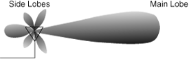
Figure 2.4. An Antenna Pattern in a Spherical Coordinate System
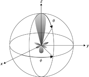
Figure 2.5. An Antenna Power Pattern Plotted versus θ for a Fixed Value of Φ
Example
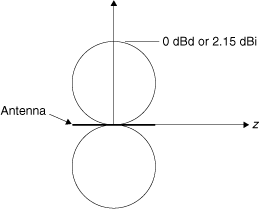
A "half-wave dipole" or just "dipole" is a very simple but practical antenna. It is made from a length of wire a half-wavelength long, fed in the center by a source. Figure 2.6 shows a schematic representation of a dipole antenna. A slice through the power pattern is shown in Figure 2.7. The dipole does not radiate in the directions of the ends of the wire, so the power pattern is doughnut shaped. If the wire were oriented vertically, the dipole would radiate uniformly in all horizontal directions, but not up or down. In this orientation the dipole is sometimes described as having an "omnidirectional" pattern. The peak power density, in any direction perpendicular to the wire, is 2.15 dB greater than the power density obtained from an isotropic antenna (with all measurements made at the same distance from the antenna). Dipole antennas are often used for making radiation measurements. Because a dipole is a practical antenna, whereas an isotropic antenna is only a hypothetical construct, power patterns of other antennas are often normalized with respect to the maximum power density obtained from a dipole. In this case the power pattern will be labeled in dBd. Measurements expressed in dBd can easily be converted to dBi by adding 2.15 dB.

Figure 2.7. Power Pattern of a Dipole Antenna
The antenna beamwidth along the main lobe axis in a specified plane is defined as the angle between points where the power density is one-half the power density at the peak, or 3 dB down from the peak. This is known as the "3 dB beamwidth" or the "half-power beamwidth" as shown in Figure 2.8. This terminology is analogous to that used in describing the 3 dB bandwidth of a filter. The "first null-to-null beamwidth," as shown in the figure, is often another parameter of interest.
Figure 2.8. Half-Power and First Null-to-Null Beamwidths of an Antenna Power Pattern

Since a power pattern is a three-dimensional plot, beamwidths can be defined in various planes. Typically the beamwidths in two orthogonal planes are specified. Often the two planes of interest are the azimuth and elevation planes. In cellular telephone systems, where all of the transmitters and receivers are located near the surface of the Earth, the beamwidth in the azimuth plane is of primary interest. The azimuth-plane beamwidth is shown in Figure 2.8.
The physics governing radiation from an antenna indicates that the narrower the beamwidth of an antenna, the larger must be its physical extent. An approximate relationship exists between the beamwidth of an antenna in any given plane and its physical dimensions in that same plane. Typically beamwidth in any given plane is expressed by
where L is the length of the antenna in the given plane, λ is the wavelength, and k is a proportionality constant called the "beamwidth factor" that depends on the antenna type. A transmitting antenna with a narrow "pencil" beam will have large physical dimensions. This implies that if the same antenna were used for receiving, it would have a large effective aperture Ae.
Example
The relation between beamwidth and effective aperture is easiest to visualize for parabolic antennas such as the "dish" antennas that are used to receive television signals from satellites. For a parabolic dish antenna, the term large aperture means that the dish is large, or, more precisely, that it has a large cross-sectional area. It is easy to see that when used for receiving, a large parabolic antenna will capture more power than a small one will. On the other hand, should the dish be used for transmitting, a large parabola will focus the transmitted power into a narrower beam than a small one.
Beamwidth is one parameter that engineers use to describe the ability of an antenna to focus power density in a particular direction. Another parameter used for this same purpose is antenna gain. The gain of an antenna measures the antenna's ability to focus its input power in a given direction but also includes the antenna's physical losses. The gain G is defined as the ratio of the peak power density actually produced (after losses) in the direction of the main lobe to the power density produced by a reference antenna. Both antennas are assumed to be supplied with the same power, and both power densities are measured at the same distance in the far field. A lossless isotropic antenna is a common choice for the reference antenna. To visualize the relationship between gain and beamwidth, consider the total power radiated as being analogous to a certain volume of water enclosed within a flexible balloon. Normally, the balloon is spherical in shape, corresponding to an antenna that radiates isotropically in all directions. When pressure is applied to the balloon, the regions of greater pressure are compressed, while the regions of lesser pressure expand; but the total volume remains unaltered. Similarly, proper antenna design alters the antenna power pattern by increasing the power density in certain directions with an accompanying decrease in the power density in other directions. Because the total power radiated remains unaltered, a high power density in a particular direction can be achieved only if the width of the high-power-density beam is small.
Beamwidth, antenna gain, and effective aperture are all different ways of describing the same phenomenon. (Technically, gain also takes into account ohmic losses in the antenna.) It can be shown that the gain is related to the effective antenna aperture Ae in the relationship[2]

where the losses are represented by the parameter η. For most telecommunications antennas the losses are small, and in the following development we will usually assume η = 1. The gain given by Equation (2.6) is referenced to an isotropic radiator.
Example
Suppose an isotropic radiator is emitting a total radiated power of 1 W. The receiving antenna has a gain described by Equation (2.6) with η = 1. Compute the required effective aperture of a receiving antenna at 10 km that will produce the same power Pr at the receiver input as would be produced by a receiving antenna with an effective aperture of Aer1 = 1 cm2 at a distance of 1 km.
Solution
The power density of the transmitted wave is given by Equation (2.2). As we showed in a previous example, p1 = 80 x 10-9 W/m2 at d = 1 km and p2 = 800 x 10-12 W/m2 at d = 10 km. According to Equation (2.3), the total power produced at the receiver input is the power density multiplied by the effective receiving antenna aperture. Thus, for the antenna at 1 km,

Now at d = 10 we have

Solving gives Aer2 = 0.01 m2. This equals an area of 100 cm2, a much larger antenna. Since gain is proportional to effective area, the second antenna requires 100 times the gain of the first in this scenario, or an additional 20 dB. Note that we could have predicted these results simply by realizing that the power density falls off as the square of the range.
Example
Continuing the previous example, suppose the communication link operates at a frequency of 10 GHz. Find the gains of the two receiving antennas.
Solution
From Equation (2.1), the wavelength is  . Now using Equation (2.6) with η = 1 gives
  or
or  . Similarly,
 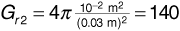 or
or  .
.
It is very important to keep in mind that although an antenna has "gain," the antenna does not raise the power level of a signal passing through it. An antenna is a passive device, and when transmitting, its total radiated power must be less than or equal to its input power. The gain of an antenna represents the antenna's ability to focus power in a preferred direction. This is always accompanied by a reduction in the power radiated in other directions. To a receiver whose antenna lies in the direction of the transmitter's main beam, increasing the transmitting antenna's gain is equivalent to increasing its power. This is a consequence of improved focusing, however, and not a consequence of amplification. Increasing the receiving antenna's gain will also increase the received power. This is because antenna gain is obtained by increasing the antenna's effective aperture, thereby allowing the antenna to capture more of the power that has already been radiated by the transmitter antenna.
It should be apparent from our discussion to this point that both transmitting and receiving antennas have gain, and both receiving and transmitting antennas have effective apertures. In fact, there is no difference between a transmitting and a receiving antenna; the same antenna can be used for either purpose. An important theorem from electromagnetics shows that antennas obey the property called reciprocity. This means that an antenna has the same gain when used for either transmitting or receiving, and consequently, by Equation (2.6), it has the same effective aperture when used for either transmitting or receiving as well.
Earlier we stated that under ideal conditions, and assuming an isotropic transmitting antenna, the power received at the output of the receiving antenna is given by
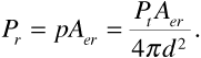
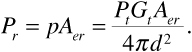
This relationship assumes that all of the power supplied to a transmitting antenna's input terminals is radiated and all of the power incident on a receiving antenna's effective aperture is captured and available at its output terminals. If we now utilize a directional transmitting antenna with gain Gt, then the power received in the direction of the transmitting antenna main lobe is given as
The term effective isotropic radiated power (EIRP) is often used instead of PtGt. EIRP is the power that would have to be supplied to an isotropic transmitting antenna to provide the same received power as that from a directive antenna. Note that a receiver cannot tell whether a transmitting antenna is directive or isotropic. The only distinction is that when a directive antenna is used, the transmitter radiates very little power in directions other than toward the receiver, whereas if an isotropic antenna is used, the transmitter radiates equally in all directions.
Example
A transmitter radiates 50 W through an antenna with a gain of 12 dBi. Find the EIRP.
Solution
Converting the antenna gain from decibels,  Then EIRP = 50 x 15.8 = 792 W.
Using the definition of EIRP, we can write Equation (2.10) as

Since the gain and effective aperture of an antenna are related by Equation (2.6), and since the gain and effective aperture are properties of the antenna that do not depend on whether the antenna is used for transmitting or receiving, it is not necessary to specify both parameters. Antenna manufacturers frequently list the antenna gain on specification sheets. If we replace Aer in Equation (2.11) using Equation (2.6) we obtain
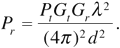
In applying Equation (2.6) we have set the loss parameter η = 1 for simplicity. We will include a term later on to account for antenna losses as well as losses of other kinds. It is instructive to write Equation (2.12) in the following way:

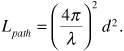
This form suggests that the received power can be obtained by starting with the transmitted power and multiplying by three "gain" terms. Since the reciprocal of gain is "loss," we can interpret the term (4π)2(d/λ)2 as a loss term. Let us define the free-space path loss Lpath as
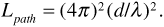
It should be observed that the free-space path loss Lpath varies directly with the square of the distance and inversely with the square of the wavelength. We can interpret the ratio d/λ in Equation (2.14) to mean that path loss is a function of the distance between transmitting and receiving antennas measured in wavelengths. It is important to note that the path loss is not an ohmic or resistive loss that converts electrical power into heat. Rather, it represents the reduction in power density due to a fixed amount of transmitted power spreading over an increasingly greater surface area as the waves propagate farther from the transmitting antenna; that is, just as G represents focusing and not actual "gain," Lpath represents spreading and not actual "loss."
Equation (2.12), the so-called range equation, can be written in any of the alternate forms

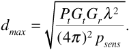
The first of these forms is known commonly as the Friis transmission equation in honor of its developer, Harald T. Friis[3] (pronounced "freese"). Subsequently we will see that there is a minimum received power that a given receiver requires to provide the user with an adequate quality of service. We call that minimum power the receiver sensitivity psens. Given the receiver sensitivity, we can use Equation (2.15) to calculate the maximum range of the data link for free-space propagation, that is,
In our analysis so far we have ignored any sources of real loss, that is, system elements that turn electrical power into heat. In a realistic communication system there are a number of such elements. The transmission lines that connect the transmitter to the antenna and the antenna to the receiver are slightly lossy. Connectors that connect segments of transmission line and connect transmission lines to antennas and other components provide slight impedance mismatches that lead to small losses. Although the loss caused by one connector is usually not significant, there may be a number of connectors in the transmission system. We have mentioned above that antennas may produce small amounts of ohmic loss. There may also be losses in propagation, where signals pass through the walls of buildings or into or out of automobiles. In mobile radio systems there can be signal absorption by the person holding the mobile unit. And so on. Fortunately it is easy to amend the range equation to include these losses. If L1, L2, ..., Ln represent real-world losses, then we can modify Equation (2.15) to read
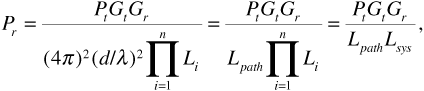
where in the last form we have lumped all of the real-world losses together into a single term Lsys, which we call "system losses."
In typical applications, signal levels range over many orders of magnitude. In such situations it is often very convenient to represent signal levels in terms of decibels. Recall that a decibel is defined in terms of a power ratio as

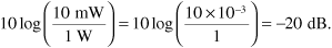
where P1 and P2 represent power levels, and the logarithm is computed to the base 10. For example, if the signal power is 1 W at 1 mile, and 10 mW at 10 miles, then the ratio in decibels is
Absolute power levels (as opposed to ratios) can also be expressed in decibels, but a reference power is needed for P1 in Equation (2.18). Reference values of 1 W and 1 mW are common. When a 1 W reference is used, the units are written "dBW" to reflect that fact; when a 1 mW reference is used, the units are written as "dBm." Expressing quantities in decibels is particularly useful in calculating received power and in any analysis involving the range equation. This is because the logarithm in the decibel definition converts multiplication into addition, and as a result the various gain and loss terms can be added and subtracted. Converting Equation (2.17) to decibels gives

Notice particularly the way in which the 1 mW reference power is handled in Equation (2.20). The reference power is needed as a denominator to convert the transmitted power Pt into decibels. The gain and loss terms are all ratios of powers or ratios of power densities and can be converted to decibels directly, without need for additional reference powers.
To make the dependence of received signal power on range explicit, let us use Equation (2.14) to substitute for Lpath in Equation (2.20). We have
The exponent of distance d in Equation (2.21) is called the path-loss exponent. We see that the path-loss exponent has the value of 2 for free-space propagation. The path-loss exponent will play an important role in the models for propagation in real-world environments that will be discussed in detail in Chapter 3. Converting Equation (2.21) to decibels gives

We see that in free space, the path loss increases by 20 dB for every decade change in range. Substituting Equation (2.22) into Equation (2.20) gives

where all of the constant terms have been lumped together as K. Note that Equation (2.23) is a straight line when plotted on semilog scale.
Example
A transmitter at 1900 MHz produces a power of 25 W. The transmitting antenna has a gain of 15 dBi and the receiving antenna has a gain of 2.15 dBi. System losses are 3 dB. If the range between transmitting and receiving antennas is 10 km, find the received signal power.
Solution
In decibels the transmitted power is  . The wavelength at 1900 MHz is given by Equation (2.1) to be
 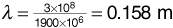 . The path loss can then be found from Equation (2.22) as
  . Now Equation (2.20) gives
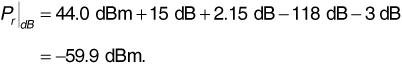
Note that system losses of 3 dB mean that half of the transmitted power is turned into heat before it can reach the receiver.
Example
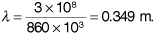
Suppose a transmitting base station emits an EIRP of 100 W. The handset receiver has a sensitivity of  . What is the maximum range for the mobile unit given the following selected antennas: a dipole having gain of 2.15 dBi, and an omnidirectional having gain of 0 dBi? The operating frequency is 860 MHz. Neglect system losses.
Solution
When working problems with the range equation, it is important to take the proper approach. In this problem, most of the data is given in decibel units, so it would make sense to start with a form of the range equation expressed in decibel units, such as Equation (2.20). Expressed in decibels, the EIRP is  . Recall that EIRP = PtGt, so in decibels,
  . Substituting into Equation (2.20) gives
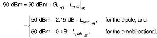
Solving for path loss gives
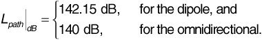
Now the wavelength λ is given by Equation (2.1):
Substituting in Equation (2.22) gives

Solving for range gives

A 2.15 dB difference in antenna gain can make a big difference in range (28% in this free-space example).
All communication systems, wired or unwired, are affected by unwanted signals. These unwanted signals are termed either noise or interference. There are no clear and universal definitions that distinguish noise from interference. Most often the term interference refers to unwanted signals entering the passband of the desired system from other systems that intentionally radiate electromagnetic waves. An intentional radiator is any radio system that uses electromagnetic waves to perform its function. The term noise often refers to unwanted signals arising from natural phenomena or unintentional radiation by man-made systems. Examples of natural phenomena that produce noise are atmospheric disturbances, extraterrestrial radiation, and the random motions of electrons. Examples of man-made unintentional radiators that produce noise are power generators, automobile ignition systems, electronic instruments, and microwave ovens. The distinction between noise and interference will become more evident when we discuss interference management in cellular systems.
The effects of interference and certain types of noise can often be mitigated and sometimes eliminated by appropriate engineering techniques and/or the establishment of rules to restrict both intentional and unintentional radiation. One particular type of electrical noise, however, is ubiquitous insofar as it arises in the very components used to implement a system. This noise, called thermal noise, arises from the thermal motion of electrons in a conducting medium and is present in any circuit consisting of resistive elements such as wires, semiconductors, and, of course, resistors. It is, therefore, present in any system that uses these components. The presence of thermal noise limits the sensitivity of all electronic wireless systems. Sensitivity is a measure of a system's ability to reliably detect a signal.
In addition to assuming that waves propagate in free space, our development of the range equation tacitly assumed ideal transmit and receive antennas and a lossless connection between the receive antenna and an ideal receiver. Under these optimal conditions there is no minimum limit to a receiver's ability to detect a signal, and therefore the operating range of such a system is limitless. Real antennas, receivers, and interconnecting circuits, however, all have resistive (lossy) elements and electronic components. These elements and components introduce thermal noise throughout a receiver and in particular in its front end, that is, the first stages immediately following the receiving antenna. When the information-carrying signal is comparable to the noise level, the information may become corrupted or may not even be detectable or distinguishable from the noise. The maximum range is, therefore, constrained by the need to maintain the information-carrying signal at some level relative to the noise level at the input to the receiver. This noise level is often called the noise floor.
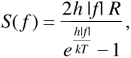
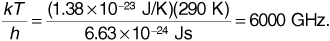
Taking into account the thermodynamic nature of the phenomenon, the noise generated by a resistor has a normalized power spectrum[4] given by
where
R is the resistance of the noise source in ohms
T is the absolute temperature in kelvin
f is frequency in hertz
k is Boltzmann's constant (1.38 x 10⁻²³ J/K)
h is Planck's constant (6.63 x 10⁻²⁴ Js)
Example
If we take T = 290 K (that is, 62.6°F, a chilly "room" temperature), then
All radio frequencies (but not optical frequencies) in use today are significantly below this value. Then for  we can write

Thus at practical radio frequencies Equation (2.29) becomes

which is independent of frequency. The units of normalized power spectrum are JΩ or, more appropriately, V2/Hz.
Noise having a power spectrum that is constant at all frequencies is called "white" noise, by analogy with white light, which has a constant power spectrum at all wavelengths. Equation (2.32) shows that thermal noise can be modeled as white noise for all radio frequencies of current practical interest. We often write the power spectrum of white noise as

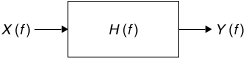
when we do not want to imply that the noise was necessarily generated by a resistor. Figure 2.9 shows a signal x(t) with Fourier transform X(f) passing through a filter with frequency response H(f). The output signal y(t) has Fourier transform Y(f). We know that
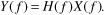
Figure 2.9. A Signal Is Passed through a Filter
Taking the magnitude squared of both sides of Equation (2.34) gives a relation between the energy spectrum of the input signal and the energy spectrum of the output signal:

Now noise does not have an energy spectrum, but it can be shown that an equation similar to Equation (2.35) applies to noise power spectra. Thus, if noise x(t) having a power spectrum Sx(f) is passed through the filter, then the power spectrum Sy(f) of the output noise y(t) is given by

Example
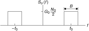
Suppose x(t) is white noise with power spectrum  Suppose the filter is a bandpass filter having the frequency response H (f) shown in Figure 2.10. Then the output noise y(t) has power spectrum Sy(f) given by
  . This power spectrum is shown in Figure 2.11.
Figure 2.10. Frequency Response of an Ideal Bandpass Filter of Center Frequency f0 and Bandwidth B
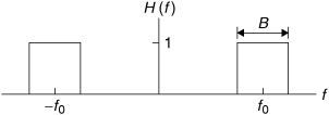
Figure 2.11. Power Spectrum of Noise at the Bandpass Filter Output
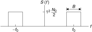
The average noise power at the filter output is the area under the power spectrum, that is,

Equation (2.37) shows that the average power in a noise signal depends not only on the spectral level N0/2 of the noise, but also on the bandwidth through which the noise is measured. It is important to emphasize that Equation (2.37) cannot be used to calculate the average noise power at the input to the filter. The unfiltered white noise at the filter input will appear to have an infinite power owing to its unlimited bandwidth. The fact that the noise power seems to be infinite is an artifact of the white noise model. As can be seen from Equation (2.29), the thermal noise power spectrum is not actually constant at all frequencies, and so thermal noise does not actually have infinite average power.
Equation (2.37) gives the average power of a white noise signal measured using an instrument of bandwidth B. If the noise is actually thermal noise generated by a resistor, then Equation (2.32) gives us

and

We need to be more precise about the meaning of the term average power, as several notions of average power will be used in the sequel. If x(t) is a signal, the average power is given by

This is actually the mean square value of x(t) or the average power that a voltage or current x(t) would deliver to a 1-ohm resistor. The average power Px is sometimes referred to as the "normalized" power in x(t) and is sometimes written <x2(t)> to emphasize the mean-square concept. We note that the square root of the mean-square value is the RMS value, so
J. B. Johnson of the Bell Telephone Laboratories was the first to study and model thermal noise (also known as "Johnson" noise) in the late 1920s. In his model, thermal noise arising from a resistance of value R is represented as an ideal voltage source in series with a noiseless resistance of value R as shown in Figure 2.12. The mean-square open-circuit voltage of the ideal voltage source is given by Equation (2.39).
Figure 2.12. Thermal Noise Model of a Resistor
Example
Suppose we have an R = 100 kΩ resistor at "room" temperature T = 290 K. Suppose we measure the open-circuit voltage across the resistor using a true-RMS voltmeter with a bandwidth of B = 1 MHz. Then

This gives

As was described earlier, thermal noise is generated by any lossy system, not just an isolated resistor. An interesting consequence of the thermal nature of the noise is that if we observe any passive system with a single electrical port, whatever noise there is appears to be generated by the equivalent resistance at the port. We will not attempt to prove this assertion, but we can illustrate it with several examples.
Example
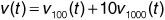
The circuit shown in Figure 2.13 consists of three resistors all in thermal equilibrium with their surroundings at temperature T. We wish to find the average power <v2(t)> in the noise voltage v(t).
Figure 2.13. A Three-Resistor Noise Source
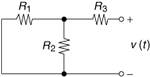
Method 1
Replace each resistor with a noise model as shown in Figure 2.12. The result is shown in Figure 2.14. This circuit can now be solved by standard circuit theory methods, say, superposition or the node-voltage method. We obtain

Figure 2.14. Resistors Replaced by Their Noise Models
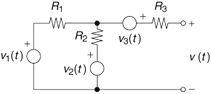
The mean-square value of v(t) is given by
where we have used the fact that the average of a sum is the sum of the averages. Now when the voltages from two distinct resistors are multiplied and averaged, we have, for example,

where we have taken advantage of the statistical independence of the voltages v1(t) and v2(t) and also of the fact that thermal noise has a zero average value. Applying Equation (2.46) to Equation (2.45) gives

We can now substitute for the mean-square noise voltages using Equation (2.39). We obtain
Method 2
As an alternate approach to finding the average power in v(t), let us replace the three resistors in Figure 2.13 with a single equivalent resistor R. To do this we first combine resistors R1 and R2 in parallel and then combine the result in series with R3. The result is
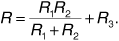
The average thermal noise power generated by the equivalent resistor R is given by Equation (2.39) as

As expected, Equation (2.50) expresses the same result as Equation (2.48), but with considerably less effort. Note that the average noise power is proportional to the measurement bandwidth B. To avoid the vagueness of a result that contains an unspecified bandwidth, we can specify the noise power spectrum rather than the average noise power. Comparing Equation (2.32) and Equation (2.39) shows that the noise power spectrum at the output of the circuit is

Example
Figure 2.15 shows a one-port passive circuit that contains a reactive element as well as a resistor. As before, the circuit is at thermal equilibrium with its surroundings at temperature T. We wish to find the power spectrum Sv(f) of the output voltage v(t) and also to find the average power Pv = <v2(t)>. As in the previous example, we will solve the problem two ways. The second solution will illustrate the "equivalent resistance" assertion.
Figure 2.15. A Noise Source Having a Reactive Element
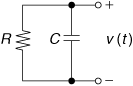
Method 1
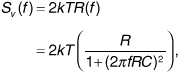
Begin by replacing the resistor with its noise equivalent as shown in Figure 2.12. The result is the circuit shown in Figure 2.16. The voltage vR(t) is the resistor noise voltage. The power spectrum of this voltage is SR(f) = 2kTR. The circuit of Figure 2.16 looks like an ideal voltage source driving an RC lowpass filter. We can, therefore, use Equation (2.36) to find the power spectrum of the noise at the output. First, the frequency response of the lowpass filter can be found by using a voltage divider. We obtain

Figure 2.16. The Resistor Is Replaced with Its Noise Model

Next, the magnitude squared of the frequency response of the filter is
Finally, we find the output-noise power spectrum, that is,

It is interesting to note that the noise at the output of the RC circuit is not white. At low frequencies the capacitor acts as an open circuit, and the noise power spectrum is essentially that of the resistor acting alone. At high frequencies the capacitor impedance becomes very small compared to the resistor and most of the noise voltage is dropped across the resistor rather than across the capacitor. The power spectrum reflects the capacitor voltage and decreases monotonically as frequency increases.
Method 2
The impedance of the circuit of Figure 2.15 as seen from the terminals is
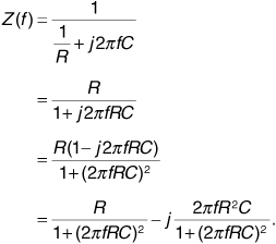
If we write

then the resistive part of this impedance is given by

Now the thermal noise at the output of the circuit appears to be generated by the equivalent resistance at the port. Substituting in Equation (2.32) gives
which is precisely the same as the answer given in Equation (2.54).
To find the average power at the circuit terminals, we can calculate the area under the power spectrum. This will give a finite result since the noise generated by the RC circuit is not white. We find
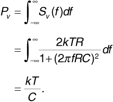
There is an interesting interpretation to Equation (2.59). If we multiply and divide by 4R, we obtain

where f3dB is the 3 dB bandwidth of an RC lowpass filter. Now refer to Figure 2.16. It appears that the average power of the noise generated by the resistor is being measured through an RC filter that sets the measurement bandwidth. If we compare Equation (2.60) with Equation (2.39), we see that the measurement bandwidth is given by

What sort of bandwidth this is will be the subject of a subsequent discussion.
Not all sources of noise are passive. Allowing amplification of the noise can produce interesting effects. An example will illustrate the idea.
Example
Figure 2.17 shows an amplifier with a room-temperature resistive noise source providing the input signal. Suppose the amplifier has a high input resistance, an output resistance of 100Ω, and a voltage gain of 10. We wish to find the average power in the output-noise signal v(t). We will consider only thermal noise in this example and will ignore any additional noise that may be contributed by transistors in the amplifier. Figure 2.18 shows the amplifier replaced by a circuit model.
Figure 2.17. An Amplifier with a Noise Source as Input
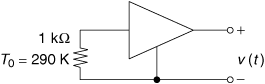
Figure 2.18. The Amplifier Is Replaced by a Circuit Model
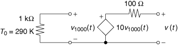
Now
where v100(t) and v1000(t) are the noise voltages across the 100 Ω and 1kΩ resistors, respectively. The average power at the amplifier output is given by
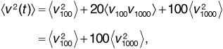
where the product of v100(t) and v1000(t) averages to zero because the noise voltages generated by physically distinct resistors are statistically independent and thermal noise has zero average value. Substituting Equation (2.42) for the mean-square resistor noise voltages gives

measured in bandwidth B.
A naive user looking back into the amplifier from the output terminals will see the Thevenin equivalent shown in Figure 2.19. The user will see a thermal noise voltage v(t) that appears to be coming from a 100 Ω resistor. The user will interpret Equation (2.64) as
Figure 2.19. Thevenin Equivalent of the Amplifier
and will conclude that the 100 Ω resistor must be at a temperature of 1001T0  290,000 K, but note details in the following discussion.
A white noise source is often characterized by a so-called noise temperature. This is the temperature at which a resistor would have to be to produce thermal noise of power (in a given bandwidth) equal to the observed noise power. The noise temperature of the circuit of Figure 2.17 is 290,000 K even though the circuit is physically at room temperature. Noise temperature is often used to characterize the noise observed at the terminals of an antenna. Antenna noise is usually a combination of noise picked up from electrical discharges in the atmosphere (static); radiation from the Earth, the sun, and other bodies that may lie within the antenna beam; cosmic radiation from space; and, of course, thermal noise from the conductive material out of which the antenna is made. At frequencies below about 30 MHz atmospheric noise is the principal component of antenna noise, and the noise temperature can be as high as 1010 K. Atmospheric noise becomes less important at frequencies above 30 MHz. A narrow-beam antenna at 5 GHz pointing directly upward on a dark night may pick up noise primarily from cosmic radiation and oxygen absorption in the atmosphere. The noise temperature in this case may be only 5 K.
Figure 2.20 shows a voltage source with a source resistance R driving a load resistance RL. This simple model might represent the output of an antenna or the output of a filter or the output of an amplifier. Two common situations arise in practice. In some circuits RL >> R and the load voltage is approximately equal to the source voltage. If the source and load voltages happen to be noise, it is meaningful to characterize these voltages by their mean-square values or, to use another term for the same quantity, by their normalized average power. A second important situation is the one in which we wish to transfer power, rather than voltage, from the source to the load. For a fixed value of source resistance R, maximum power transfer occurs when RL = R. Under this condition we have

Figure 2.20. A Signal Source Driving a Load
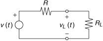
and the actual average power transferred to the load is

This quantity is called the available power.
Example
A resistor of value R at temperature T is a source of thermal noise. A model for the resistor has been given in Figure 2.12. Using Equation (2.67), we find the available noise power to be
The units of available power are watts. We can also find the available power spectrum:

The units of available power spectrum are watts per hertz. It is important to note that the available power spectrum depends only on the temperature of the source and not on the value of the resistor. This is further motivation for characterizing an arbitrary noise source by its noise temperature.
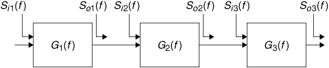
A two-port is a subsystem with an input and an output. Two-ports model devices such as filters, amplifiers, transmission lines, and mixers. In this section we develop ways to characterize the noise performance of two-ports. We are interested in describing the effect that the two-port has on noise presented at its input and are also interested in identifying the effect of noise added by the two-port itself. We will find that for noise calculations a two-port device can be characterized by three parameters: the available gain, the noise bandwidth, and the noise figure.
Figure 2.21 shows a two-port connected in a circuit. The two-port is driven by a source having source resistance Rs and the two-port in turn drives a load of resistance RL. Suppose that the source available power spectrum is Ss(f). Note that this available power spectrum characterizes the power that could be drawn from the source into a matched load. Although communication systems are often designed so that the input impedance of a two-port such as that shown in the figure is matched to the source resistance, this is not necessarily the case. That means that the source available power spectrum may not represent the power that is actually absorbed by the two-port device. Let us suppose further that the load available power spectrum is So(f). Again, the actual load resistor RL may or may not be matched to the output resistance of the two-port. The load available power spectrum may not characterize the power actually delivered to the load. Now the available gain G(f) is defined as
Figure 2.21. A Two-Port with a Source and a Load
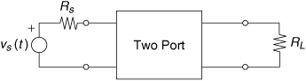
As the ratio of two power spectra, the available gain is a kind of power gain. Note that the available gain is a function of frequency. Some two-ports, such as transmission lines and broadband amplifiers, have available gains that are relatively constant over a broad frequency range. Other two-ports, such as filters and narrowband amplifiers, have available gains with a bandpass characteristic; that is, the available gains are constant over a narrow range of frequencies and very small otherwise. We will normally be interested only in the available gain in the passbands of such devices.
Figure 2.22 shows a cascade of three two-ports. Suppose the two-ports have individual available gains G1(f), G2(f), and G3(f) respectively, and we wish to find an expression for the overall available gain G(f) of the cascade. The available power spectrum at the input and output of each individual two-port is indicated in the figure. Note that the available power spectrum at the output of stage 1 is identical to the available power spectrum at the input to stage 2. Likewise, the available power spectrum at the output of stage 2 is identical to the available power spectrum at the input to stage 3. We have

Figure 2.22. Cascaded Two-Ports
Thus, two-ports can be combined in cascade simply by multiplying their available gains. The usefulness of the available gain concept can be seen in the following example.
Example
A two-port with available gain G(f) is driven by a white noise source having available power spectrum  . At the output of the two-port we have

The available noise power at the output is the area under the available power spectrum, that is,
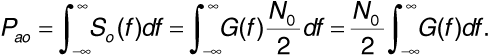
Many bandpass two-ports such as amplifiers and filters have an approximately rectangular passband. An idealization of such a passband is shown in the available gain plot of Figure 2.23. Suppose we have an actual two-port device and we model this device by adjusting the plot of Figure 2.23 so that the center frequency f0 and the midband gain G0 reflect parameter values of the actual device. Now suppose the actual device and the ideal model are both driven by identical white noise sources. The available power at the output of the actual device is given by Equation (2.73). To find the available power at the output of the ideal device we first find the available power spectrum at the output using Equation (2.72). This available power spectrum is shown in Figure 2.24. The available power at the output is the area under the available power spectrum, that is,
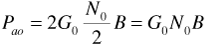
Figure 2.23. Available Gain of an Ideal Bandpass Filter
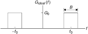
Figure 2.24. Available Power Spectrum at the Ideal Bandpass Filter Output
for the idealized model. Now we want the idealized model to predict the correct value for available power out, so Equation (2.74) and Equation (2.73) must give the same value of Pao. To make this happen, the bandwidth parameter B in the idealized model must be given by
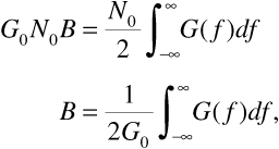
where G(f) is the available gain and G0 is the midband available gain of the actual two-port.
The bandwidth B given by Equation (2.75) is called the noise bandwidth of the actual two-port. When a two-port is characterized by a midband available gain and a noise bandwidth, available noise power at the output can be calculated by Equation (2.74), avoiding the evaluation of a sometimes messy integral. The noise bandwidth of a two-port usually has a somewhat different value from the 3 dB bandwidth and from the passband bandwidth. If the two-port has a sharp cut-off at its passband edges, however, then all of these bandwidths will have similar values.
The derivation above defined the noise bandwidth of a bandpass two-port. We can define the noise bandwidth for a lowpass two-port in an analogous way, as is shown in the following example.
Example
Consider an nth-order lowpass Butterworth filter, for which the available gain is

where f3dB is the 3 dB bandwidth. Note that the DC gain of this filter is unity. Then

For n =1 we have  (compare Equation (2.61)). As n → ∞ we find B → f3dB.
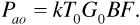
Now consider a physical amplifier with available gain G0 and noise bandwidth B driven by a room-temperature noise source. The arrangement is shown in Figure 2.25.
Figure 2.25. A Two-Port with a Room-Temperature Noise Source
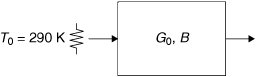
According to Equation (2.74), the available noise power at the amplifier output should be Pao = G0N0B. In fact, the output power will be larger than this owing to noise generated within the amplifier. There are two widely used conventions for accounting for this additional noise, the noise figure and the effective input-noise temperature. Noise figure is the older of the two conventions; it is widely used in terrestrial wireless systems. Effective input-noise temperature is more common in specifying satellite and other space systems that operate with extremely low antenna noise temperatures. We will introduce noise figure first and then we will present the effective input-noise temperature alternative.
Suppose, in the setup shown in Figure 2.25, the available power actually obtained at the output of the two-port is Pao. Then the noise figure is defined as

where G0 and B are the available gain and noise bandwidth respectively, that is,
It is important to note that Equation (2.79) is valid only when the noise source is at room temperature T0 = 290 K. It is common practice to express the noise figure in decibels, where

In some texts, F is called the noise factor and the term noise figure is reserved for FdB. Since a two-port can add noise, but not subtract noise, the noise figure F is always at least unity. This means that the noise figure in decibels FdB is never negative. If we rewrite Equation (2.79) as

we recognize the first term kT0G0B as the output-noise power caused by the room-temperature source. This means that the second term
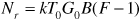
must be the noise power contributed by the two-port. If the noise source were at some temperature T other than room temperature, then the first term in Equation (2.81) would change, but the second would not. In general, for a source of noise temperature T we have

To help develop some intuitive feeling for the noise figure concept, let us consider the effect of two-port noise on signal-to-noise ratio. We shall see in subsequent chapters that signal-to-noise ratio is an important figure of merit for system performance. Suppose a two-port such as the one shown in Figure 2.25 receives a signal of available power Psi at its input. We will assume that the room-temperature white noise is also present. Assuming that the signal is within the passband of the two-port, the signal power at the output is given by

Since the output-noise power is given by Equation (2.79), we can write the signal-to-noise ratio at the output as
We would like to compare the signal-to-noise ratio at the two-port output with a similar ratio at the two-port input. At the input, however, the noise is white and the total noise power cannot be calculated. (Our white noise model would give a total input-noise power of infinity.) To allow the comparison, let us define an "input-noise power" that is the noise power in the bandwidth B. This is a plausible step, since only noise within the passband of the two-port will make its way through the two-port to the output. The input-noise power calculated this way is

Using this definition of input-noise power, we can find the input signal-to-noise ratio,

We can calculate the degradation in signal-to-noise ratio caused by the two-port if we take the ratio of SNRi to SNRo. We obtain

which is just the noise figure.
A low-noise amplifier will have a noise figure very close to unity. An alternative way of representing two-port noise that is useful in this case is the effective input-noise temperature Te. In this formulation we refer again to Figure 2.25, only in this case we do not require the input-noise source to be at room temperature. We write the available noise power at the output as

where T is the noise temperature of the source. Comparing Equation (2.89) with Equation (2.81), we can write
Pao = kTG0B + Nr,
where kTG0B is the available noise power at the output due to the input-noise source, and Nr is the available noise power at the output contributed by the two-port. We have

Example
Figure 2.26 shows a receiver "front end." This includes the amplifiers, mixers, and filters from the antenna to the demodulator. The antenna is shown as a source of noise having noise temperature Tant = 10 K.
Figure 2.26. Receiver Front End
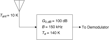
Now the available noise power spectrum from the antenna is
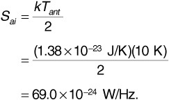
(We avoid calculating the available input-noise power.)
To include the amplifier noise, the output-noise power spectrum uses a temperature of Tant + Te = 10 + 140 = 150 K, that is,

We must also convert the available gain from decibels:  Then the available output-noise spectrum is

The available output-noise power is

Noise figure and available input-noise temperature are measures of the same quantity. Thus, Equation (2.82) and Equation (2.90) must give the same value for Nr. Then
Solving for Te gives
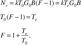
Figure 2.27 shows a system made up of a cascade of three noisy two-ports. In an actual receiver these might be, for example, a low-noise amplifier, a transmission line, and a high-gain amplifier-filter. Each of the individual stages is characterized by an available gain and a noise figure. We assume that one of the stages limits the bandwidth of the cascade, and we use the symbol B to represent that bandwidth. Our object is to combine the three stages and obtain an equivalent single two-port having an available gain G0, a noise figure F, and bandwidth B.
Figure 2.27. A Cascade of Noisy Two-Ports
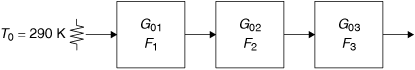
We already know from Equation (2.71) that the combined available gain is

To ensure the proper use of noise figure, the input to the cascade is a noise source at room temperature T0 = 290 K.
The available noise power at the output of the cascade is the sum of the noise power contributed by the source plus the noise power contributed by each individual stage. We can write

where the noise from each stage is amplified by the stages that follow it. Using Equation (2.82), we obtain

Now for the equivalent single two-port,

with G0 given by Equation (2.97). Equating Equation (2.99) to Equation (2.100) and dividing by kT0G0B gives
The extension to an arbitrary number of stages should be obvious.
If we wish to work with effective input-noise temperature rather than with noise figure, then we can substitute Equation (2.90) into Equation (2.98) to obtain

where Te1, Te2, Te3 are the effective input-noise temperatures of the three stages respectively. For the equivalent single two-port,
As before, we equate Equation (2.102) to Equation (2.103) to obtain
Equations (2.101) and (2.104) are sometimes known as Friis formulas, after Harald Friis, who developed the theory of noise figure at the Bell Telephone Laboratories in the 1940s. (This is the same Friis who brought you the Friis transmission formula!)
Equation (2.101) (or Equation (2.104)) contains an important message. If the three stages have comparable noise figures, then the dominant term in Equation (2.101) will be the first term. This suggests that if the first stage of a receiver has a low noise figure and a high gain, then the noise figures of the subsequent stages do not matter much. It is common practice for the first stage in a receiver to be a "low-noise" amplifier (LNA).
Example
Figure 2.28 shows the first two stages in a receiver. The first stage is a low-noise amplifier, and the second stage is a mixer. The available gains and noise figures are as given in the figure. The antenna noise temperature is also specified. No bandwidth is given in this example, as the bandwidth-limiting stage would normally be the intermediate-frequency (IF) amplifier that would follow the mixer.
Figure 2.28. The First Two Stages in a Receiver
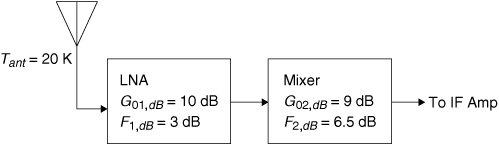
The overall gain of the system is given by

We must begin the noise analysis by converting the gains and noise figures from decibels. We obtain G01 = 10 and F1 = 2 for the LNA, and G02 = 8 and F2 = 4.47 for the mixer. Next we can find the overall noise figure from Equation (2.101):
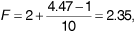
or

Notice how close the overall noise figure is to the noise figure of the LNA.
Since the input noise is not coming from a room-temperature source, we cannot use the overall noise figure to find the available output-noise power spectrum directly. One alternative approach is to use the effective input-noise temperature, which does not presume the use of a room-temperature noise source. From Equation (2.96) we obtain

Then

A transmission line is a coaxial cable or waveguide used to connect a transmitter or a receiver to an antenna and sometimes to connect other stages in a communication system. Transmission lines are lossy, particularly at the frequencies used in cellular and personal communication systems. Consequently the losses of the transmission line must be taken into account in any system design. Losses in the receiving system are particularly damaging, as losses are a source of thermal noise.
Let us consider a length of transmission line of characteristic impedance Z0. In most practical circumstances we can take Z0 to be a real number. We will look at a transmission line from two points of view. First, a transmission line is a two-port, and therefore it has an available gain and a noise figure. We note, however, that the available gain will be less than unity. Expressed in decibels, the available gain will be a negative number. It is customary to drop the minus sign and describe the transmission line in terms of its loss; that is, letting G represent the gain and L represent the corresponding loss,

and
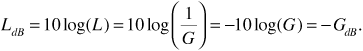
Now suppose the transmission line is terminated at its input end in a resistor of value R = Z0. We will assume that the input resistor, and in fact the entire transmission line, is in thermal equilibrium at room temperature T0. Figure 2.29 shows the setup. The available noise power at the output of the transmission line is

Figure 2.29. A Lossy Transmission Line at Room Temperature
measured in bandwidth B.
For our second point of view we will take the transmission line with the input resistor connected to be a one-port circuit. We observe that since the input resistance equals the characteristic impedance of the transmission line, the impedance seen looking into the output end of the line is Z0, which we are taking to be a real number. Now recall that for a passive circuit, whatever noise there is, appears to be generated by the equivalent resistance at the port. This means that the available power at the output of the transmission line is just the power generated by a room-temperature resistor. We have

Now Equation (2.112) and Equation (2.113) describe the same quantity. Equating these gives us the noise figure of the lossy line:

As an intuitive description of the operation of a lossy transmission line, consider what happens when a signal in room-temperature noise is introduced at the input of the line. The signal is attenuated in passing down the transmission line. The input noise is attenuated also, but the transmission line adds noise of its own, to exactly make up the noise that is lost. At the output, then, we have a reduced signal that is still in room-temperature noise. The signal-to-noise ratio is reduced in the transmission line by exactly the loss in the signal. If the noise figure represents the degradation in signal-to-noise ratio, we are led immediately to Equation (2.114).
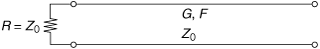
As a practical example of applying these concepts, we calculate the noise figure and effective input-noise temperature for the front end of a mobile telephone receiver. The receiver is shown in Figure 2.30. In the following analysis we derive expressions for the effective input-noise temperature at each interface. Most of the components shown in the figure are straightforward, but the mixer requires a comment. Since the mixer is specified as having loss LC, a passive mixer is assumed. A passive mixer contains diodes, and so it is not a linear system. Consequently the analysis that we used to find the noise figure of a lossy transmission line cannot be applied to the mixer without some modification. It turns out, however, that for most practical mixers the noise figure is only very slightly higher than the loss. Consequently it is common practice to set F = LC for a passive mixer with only negligible inaccuracy.
Figure 2.30. The Front End of a Mobile Telephone Receiver
Let us now proceed from right to left through the receiver system:

 . Substituting gives
  .
.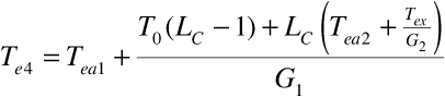
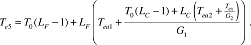
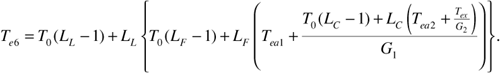 .
.LL = Antenna cable loss = 3dB (2)
G1 = LNA gain = 30dB (1000)
TeA1 = LNA noise temperature
FA2 = IFA noise figure = 1.0 dB (1.3)
LC = Mixer conversion loss = 6dB (4)
Tex = Noise temperature rest of receiver
LF = Filter loss = 3dB (2)
FA1 = LNA noise figure = 1.5dB (1.4)
G2 = IFA gain = 30dB (1000)
TeA2 = IFA noise temperature
Fx = Noise figure rest of receiver = 16dB (40)
Using these values, we compute the effective input-noise temperature at each interface, but first let us calculate the effective input-noise temperature for those components that are specified in terms of their noise figure:
The effective input-noise temperature at each interface is computed:
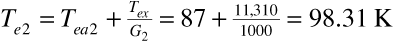

The overall effective input-noise temperature of the receiver front end, Ter, is 1339 K. It is interesting to note how low the effective input-noise temperature is at interface 4. At this point Te4 is only one degree higher than the effective input-noise temperature of the low-noise amplifier alone. Having 6 dB of transmission line and filter loss ahead of the LNA has a very deleterious effect, increasing the effective input-noise temperature by more than an order of magnitude. Clearly if noise were the only design consideration, it would make sense to place the LNA right at the antenna, ahead of the transmission line and filter.
The overall receiver noise figure is given by Equation (2.95). We have
At the start of our discussion of thermal noise we stated, "When the information-carrying signal is comparable to the noise level, the information may become corrupted or may not even be detectable or distinguishable from the noise." It might at first seem plausible, then, that, given a fixed receiver noise level, a key objective of our radio link design should be to maximize the information-carrying signal power delivered to the receiver. On further reflection, however, we see that this is not precisely the case. For any communication system, the most important goal is to ensure that the user is provided with an adequate quality of service. For a telephone connection, the received voices should be intelligible, and the identity of the speaker should be discernible. Calls should not be interrupted or dropped. For a data connection the received data should be accurate and timely. Images should be clear, crisp, and with good color. Music should have good fidelity and there should be no annoying hisses or whines in the background. Stating design goals in terms of user perceptions, however, raises immediate issues about what is meant by "intelligible," "accurate," "clear," and "good fidelity." Not only must all of these "quality" terms be quantified, but they must also be expressed in terms of parameters that engineers can control. To guarantee intelligibility and fidelity, we must provide a certain bandwidth and dynamic range. To guarantee accuracy and timeliness, we must provide a low rate of data errors. Systems engineers describe the engineering parameters that directly affect user perceptions as quality of service (QoS) parameters. In a digital transmission system, several QoS parameters are related to a particularly important parameter of the data link, the bit error rate (BER), which is a measure of how often, on the average, a bit is interpreted incorrectly by the receiver. In a later chapter we will show that bit error rate is directly related to the ratio of the received signal level to the noise and interference level at the receiver's input terminals. Thus the design goals are more appropriately stated like this: To provide intelligible voice, or clear images, there will be a maximum acceptable bit error rate. To achieve this bit error rate, there will be a minimum acceptable signal-to-noise-and-interference ratio (SNIR), or just signal-to-noise in the absence of interference. We now see that a design objective that is more appropriate than maximizing received signal power is to ensure that an adequate SNR is achieved at the receiver input. Delivering more power than that required to meet this SNR objective is actually undesirable from a system perspective. In this section the reasons for using this design objective and its intimate relation to link design are investigated.
For discussion purposes, we consider our system as a basic radio link, that is, a system consisting of a transmitter and receiver, with intervening free space as the channel. To optimize the performance of this link, we must first determine the specific performance objectives to be optimized, and we must then identify all of the relevant parameters affecting these performance objectives. For a wireless system, particularly a mobile system such as a cellular telephone, cost and size, weight, and power are equally important as SNR. Optimization, then, has much broader scope than many other technical treatments might consider. From a systems-engineering point of view, optimization should be holistic, considering not only how well a system operates but also all of the other relevant attributes that might constrain a design. For example, designers should consider battery life and portability as constraints for optimizing the more common performance objectives such as data rate and bit error rate.
System design, then, is a process of optimizing a system's technical performance against desired and quantifiable constraints, such as cost, size, weight, and power. So, from a systems engineer's point of view, the design problem should be restated, "Given all of the system constraints, how do we guarantee that an adequate SNR is delivered to the receivers via the radio links?" (Yes, there are two links, forward and reverse, and they are not symmetric.) Given the importance of features such as size, weight, cost, and battery life, maximizing the power delivered to a receiver without considering constraints on these other features is not a well-founded design objective. The consequences of transmitting more power than necessary will certainly affect all of the system attributes as well as contribute to the overall background of RF energy, thereby causing unnecessary interference.
As stated previously, the measures of goodness or QoS provided by a system are often related to the SNR. At this point in our study, however, we will not discuss the relationships quantitatively. For the present discussion, it is sufficient to assume that if the SNR is adequate, the relevant QoS objectives will be met. In later chapters we will show how the choice of modulation and signaling type is related to SNR. Understanding the relationships allows a link analyst to determine the SNR required to achieve a given level of performance. For a digital system, a typical performance parameter might be bit error rate at a particular transmission rate (e.g., a BER of 10-7 at 100 kbits/s), a parameter of particular interest at the most basic level of analysis.
A simplified description of a typical RF link design process is as follows. Once the key link performance parameters are identified and detailed objectives are established (bit error rate, data rate, etc.), a signaling scheme is chosen. Given a chosen signaling scheme, the required baseband SNR is calculated and adjusted for the implementation loss of the actual receiver. The result is a prediction of the actual SNR that the receiver requires to achieve the performance objectives. Noise power levels are calculated for typical operating environments and are then translated back to the receiver input to produce a prediction of the required SNR at the input to the receiver. (If interference is present, we also calculate the interference power levels to determine the required signal-to-noise-and-interference ratio at the input to the receiver.) Given the SNR and noise power, the corresponding minimum required power psens at the input to the receiver is then calculated. The power psens is known as the receiver sensitivity and is the minimum power required to meet the given performance objective (such as bit error rate or data rate). Systems engineers use the range equation to ensure that this power level is achieved over the range of interest and over all expected operating conditions.
Overdesigning the link by delivering more power than required could introduce difficulties in meeting objectives and constraints involved in the system implementation. For example, too much power radiated from an antenna could violate license parameters or even pose a health risk. Excessive power feeding the antenna will cause unnecessary battery draw in a portable unit or create excessive heat. Excessive transmitter power could also cause interference between the transmitter and receiving sections of a handheld unit, necessitating extra shielding and thus extra bulk and cost. Notwithstanding these considerations, a certain level of overdesign is usually mandated by good engineering practice: The link system engineer will provide for the delivery of the required minimum power to the receiver plus some extra power called "margin." Margin power ensures that the minimum required power is maintained in spite of design errors, aging effects, and manufacturing variations, as well as variations introduced by a real-world propagation environment, as will be discussed in the next chapter. Evidently, a systems engineer must have a good understanding of both the design objectives and system variables in order to optimize a system design to meet performance requirements within specific design constraints such as cost, size, weight, and battery life.
Given the discussion above, our design objective has been reduced to ensuring that some power Pr, which is the receiver sensitivity plus margin, is delivered to the receiver over the radio link. The range equation is the basic radio link model we developed earlier for predicting the variation in received power versus distance between a transmitter and a receiver. It is repeated here for convenience:

The range equation is expressed in terms of five variables that can be selected so that the power Pr is delivered to the receiver. Each of these variables may have design constraints that must be considered and traded off to optimize the link. For example, Gt is more than just a number representing the gain of an antenna. Its value has implications regarding the beamwidth, size and weight, and cost of an antenna. The system designer must work with subsystem and component designers to balance the performance and cost of each of the terms in implementing a solution. It is also important to note that for some applications the forward and reverse radio links may not be symmetric. For systems of interest to us the forward link, in the direction from a base station to a portable unit, looks much different from the reverse link. As such, a design must consider the requirements of each link as well as of the system as a whole. An examination of each term in the range equation will reveal how link design is performed.
First, consider the top-level link design parameters. One of the first terms to consider is actually one that is least obvious in Equation (2.115). Specifically, the operating frequency (wavelength) is woven into each of the variables of the range equation. For example, the free-space loss term Lpath is obviously wavelength dependent, varying as the inverse of wavelength squared. The antenna gain terms have wavelength dependence as well. Even the transmitter power term may have some wavelength dependence associated with the power delivery system between the transmitter's final amplifier and the transmitting antenna. In addition, the use of a radio link operating frequency is regulated by the FCC and must also be chosen to produce manageable antenna dimensions. Typically, the choice of operating frequency has as much to do with spectrum availability as with technical desirability.
Once the operating frequency is chosen, the design may proceed. As stated earlier, our goal is to produce the minimum power Pr (as specified by the minimum required SNR plus margin) at the receiver input terminals. The process of taking this initial requirement and decomposing it into specific requirements allocated to each of the various subsystems of the link is called "requirement flow-down" or "allocation." A systems engineer must have the experience and knowledge of a broad range of technologies to know how to best flow down or allocate requirements among the various subsystems. It is always good practice, however, to engage the subsystem designers to ensure that the most informed choices are made and ''buy-in'' is obtained on the requirements from the design team.
There are a number of practical considerations surrounding the transmitter and determining its transmitted power Pt. Figure 2.31 is a block diagram of a simplified transmitter RF stage, which is helpful when discussing some of the design considerations. As its name implies, the power amplifier (PA) increases the power of the signal to be transmitted to some level in excess of the desired level Pt. A matching network may be required to match the amplifier output impedance to the antenna feed, which carries the signal to the antenna. If the transmitter is a base station, the feed may be a 150-foot or longer cable, so that power loss in the cable and connections may be appreciable. The power at the output of the PA should be large enough to account for the losses in the matching network and feed system so that the power delivered to the antenna terminals is Pt as required. Of course, due care in the design and selection of these components is required to avoid wasting power, especially in a mobile unit.
Figure 2.31. Transmitter RF Stage Block Diagram
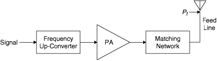
Amplifier design is important as well; an amplifier that wastes power (that is, one that has high quiescent power dissipation) is undesirable since it will drain the battery of a mobile unit. On the other hand, low quiescent power amplifiers tend to be nonlinear to some degree. In cell phones, low quiescent power amplifiers often introduce problems arising from nonlinearity of the power amplifier, which introduces unwanted frequencies in the transmitted spectrum. We will discuss this further in a later chapter on signaling. Although it is important to design matching networks and feed systems to minimize loss, wide-bandwidth, low-loss components are difficult to design and expensive to implement so that a prudent trade-off may be required between performance and cost. Therefore, a systems engineer should engage circuit designers to optimize the performance of these subsystems to ensure maximum power delivery to the antenna.
Example
Suppose a power amplifier is operated at its maximum linear power output point P1dB = 40 dBm. The matching network and connectors introduce a loss of 0.5 dB and the feed cable adds an additional loss of 3 dB. The transmitting antenna gain in the desired direction is 10 dBd. Find the EIRP for this radio transmitter.
Solution
EIRP is defined as the radiated power produced by an isotropic radiator producing the same power as the actual antenna in the desired direction. This is equivalent to calculating PtGt as defined previously, but several details must be considered first.
First, write the equation that will determine the EIRP in decibels relative to 1 milliwatt (dBm):

The first term on the right-hand side is the output power level of the power amplifier, which is given as 40 dBm. The last term is the gain of the transmitting antenna. Antenna gains are normally given in terms of either dBd or dBi references. To convert dBd to dBi, simply add 2.15 dB. This accounts for the gain of a dipole relative to an isotropic radiator. In this example, the EIRP is calculated as

Thus, the EIRP produced is 48.65 dBm or 73.3 W. (Note that another measure of radiated power is often used, the effective radiated power [ERP], which is the radiated power above that of a dipole. The ERP in this case would be 48.65 dBm - 2.15 dB = 46.65 dBm or 46.2 W.) This is a reasonable example of a single-channel radio transmitter performance for the base station of a cellular phone link. Note that a mobile unit cannot support this power level from either a battery or a heat dissipation perspective.
The transmitting antenna gain term Gt is also more than a number. Its value depends on the antenna design, dimensions, and use. For the forward link, there is greater flexibility at the base station to meet design constraints associated with the terms Pt and Gt than at the mobile unit. This reduces the need for high-gain, low-loss antennas in the mobile unit.
Similar considerations apply for the receiving antenna gain term Gr. For the mobile unit, the same antenna is used for both transmitting and receiving, and a device known as a diplexer is used to separate the signals. At the base station, separate antennas are used for transmitting and receiving, which eliminates the need for a diplexer and its associated loss.
Based on this discussion, it should be apparent that there is greater flexibility at the base station for implementing system components, especially in terms of transmit power and antenna gain. Mobile units are severely constrained by the amount of power they can radiate, the size of the antennas they can support, the volume of circuitry they can house, and the amount of heat they can dissipate. This allows the base station to "take up the slack" by providing more transmitter power in the forward direction and higher-gain antennas in both the forward and reverse links. Furthermore, since larger, higher-gain antennas and better receiver electronics can be accommodated at the base station, the return link can be designed to provide better receiver sensitivity. As a result, the mobile unit design constraints can be made less demanding.
As a first consideration, an inexperienced systems engineer might attempt to balance the forward and reverse links by making the transmitter and receiver designs equally demanding on both the base station and mobile units. Size, weight, cost, and power constraints, however, are far more difficult to meet for a mobile unit than they are for a base station. An asymmetric approach allows the apportionment of antenna gain and transmitter power in a manner that reduces the difficulty in meeting mobile unit performance requirements by shifting the "burden" to the base station where the design constraints are not as restrictive.
In this example, we will examine both the forward link (or downlink) from the base station to the mobile unit and the reverse link (or uplink) from the mobile unit to the base station. Although these links are asymmetric, there are elements in common—the link ranges will be identical and the handset antenna is the same for transmitting and receiving. The frequencies of the forward and reverse links may not be the same, but they are often very close.
For the forward link we use the transmitter and receiver architecture described previously. The reverse link will be specified in a similar manner, with the handset as the transmitter and the base station as the receiver, and with some modifications to the architecture as described. In this example we will find the maximum link range that can be achieved given the described hardware. We will assume an operating frequency of 1900 MHz.
The base station RF stage is described by the parameters listed in Table 2.1, corresponding to Figure 2.31. Note that the base station produces a higher EIRP than the handset, as would be expected from the considerations discussed above.
Table 2.1. Transmitter Parameters for Example Link Budget
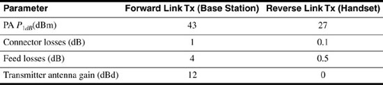
For the receiver analysis, we assume that the entire receiver has been analyzed as shown here and modeled as a single RF unit with a gain and noise figure, feeding a baseband detector as shown in Figure 2.32. The parameters for the receiver model for the forward and reverse link are given in Table 2.2. The receiver antenna gain is higher than the transmitter antenna gain for the base station owing to the common practice of using multiple receiving antennas. The base station and handset receivers are assumed to have identical gains and noise figures to simplify the example. The antenna noise temperatures for the base station and handset are different. Base station antennas are often tilted down slightly to limit interference with nearby cells. The base station antenna is thus "looking" at the Earth and sees Earth-temperature noise (290 K). The handset antenna, being small, is not very directional. It "sees" both Earth and sky and consequently will be assumed to have a lower antenna noise temperature.
Figure 2.32. Simplified Model for Receivers

Table 2.2. Receiver Parameters for Example Link Budget

We begin the analysis with the range equation, Equation (2.20), which we repeat here for convenience:

Note that we have added an additional loss term to the range equation, to allow for design margin, as described in our discussion of receiver sensitivity. For illustrative purposes we choose a design margin of 3 dB for both links. We perform the analysis twice, once for the forward link and once for the reverse link. Using the parameters of Table 2.1, we find that 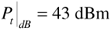 ,
,  ,
,  , and
, and  . If we can find the required signal power
  at the receiver input, we will be able to solve Equation (2.118) for the path loss. Then we can use Equation (2.22) to find the maximum range.
Determining the required signal power at the receiver input begins with a noise analysis. Since the antenna noise temperatures are not room temperature, we will use effective input-noise temperature to characterize the receivers rather than noise figure. Now a noise figure of  can be converted from decibels to a factor F = 6.31. The receiver's feedline loss of 0.5 dB implies a feedline noise figure of 0.5 dB, or Ffeed = 1.12. Combining the feedline and receiver noise figures using Equation (2.101) gives
  . Then Equation (2.96) gives Te = (Ftotal - 1) T0 = (7.08 - 1)290 = 1760 K. The noise power at the detector input is given by Equation (2.89) as

where the receiver noise temperature for the forward link is T = 60 K,  (including the feedline loss and RF unit gain of 40 dB), and B = 100 KHz. Expressed in decibels, the noise power at the detector input is

Now the required signal-to-noise ratio at the detector input is 12 dB. This means that the signal power required at the detector input is
Since the RF unit has a 40 dB gain, the signal power required at the receiver input is now determined to be

Given the required received signal power, we can substitute in the range equation and find
Once we have the maximum path loss, we are one step away from the maximum range. At a 1900 MHz frequency the wavelength is λ = 0.158 m. Then

Repeating this calculation for the reverse link, we start with the given items  ,
,  ,
,  , and
, and  . Using an antenna noise temperature of T = 290 K, we find the required signal power at the receiver input to be
  . The range equation then gives the maximum allowable path loss:
  . Finally, we can proceed as in Equation (2.124) to find the maximum range as a = 171 km.
We see from this analysis that the maximum range of the link is determined in this example by the reverse link and is d = 171 km. In practice it is usually considered desirable to adjust the forward and reverse link parameters so that the signal-to-noise ratios are the same in both cases. This gives users at both ends identical perceptions of the quality of service. The easiest way to "balance" the links is often to reduce the transmitted power in the forward link.
In this chapter the basic element of wireless communication, the radio link, was investigated. A combination of various kinds of expertise, including circuit design, antenna design, manufacturing, and basic link analysis, are utilized to "close the link" or guarantee that an adequate signal-to-noise ratio is delivered to the receiver detector. A systems-engineering approach allows for trading among the various system parameters to achieve a specific goal associated with the desired quality of service objectives.
The major topics covered in this chapter are each an introduction to a field of study. Students are encouraged to review current publications in each of the areas to obtain better understanding of each field as a prospect for specialization or to understand how recent advances can influence new designs. Suggested areas for study are
Throughout the rest of this text, many of the topics we introduced in this chapter will be refined and expanded to provide a more accurate representation of a physical radio link, thereby providing the basis for better design and prediction of radio link performance. In Chapter 3 we investigate electromagnetic wave propagation in a terrestrial environment. Our discussion will reveal that measurement, analysis, and modeling are required to account for the phenomena that influence electromagnetic transmission in natural and man-made environments.
Consider a transmitting antenna of extent L = 1 m located at the origin and aligned with the z axis of a right-hand rectangular coordinate system in free space. Two isotropic receive antennas are located at a distance of 2 km from the origin and at z = ±0.25 km above and below the x-y plane. The antenna has a beamwidth factor of 66°. What is the highest frequency that can be transmitted so that the power at the receive antennas is no less than half the peak value?
An isotropic antenna is radiating a total power of P0 W. A receive antenna is located 2 km from the radiator. It has a gain described by Equation (2.6) with loss factor η = 0.9 and an effective aperture of Aer1 = 600 cm2. How far away can a second antenna with η = 0.8 and effective aperture Aer2 = 1.0 m2 be located so that both antennas receive the same power at their output terminals?
Compute the gains of the two antennas in the previous example for the case where the transmitter frequency is 800 MHz. What are the gains if the transmit frequency is 1.9 GHz? Express your answers in dBi.
Assume that the antennas in Problem 2.3 are dish antennas such that  If the beamwidth factor for either antenna is 51°, find the beamwidth of each antenna for each frequency.
A receiver is located 5 km from a transmitter in free space. The output at the terminals of the receive antenna is -87 dBm. The receive antenna has a gain of 2 dBd and there is a total of 2.8 dB of system loss. Calculate the transmitter EIRP in watts given a transmit frequency of 890 MHz. If the transmit antenna has a gain of 7.5 dBi, what is the transmit power in watts?
A transmitter radiates an EIRP of 1 W into free space. A receive antenna located at 1 km from the transmitter has a gain of 5 dBi. Assume that there are 2 dB of system loss.
A. If the system operates at 900 MHz, what is the power level at the output of the receive antenna terminals?
B. What is the power level at the output of the receive antenna terminals if the system operates at 1800 MHz?
C. How does the received signal level vary between cases A and B?
Explain what physically causes the received power to be different in these two cases, even though all other parameters do not change.
A transmitter in free space has an output power of 5 W and operates at 1.9 GHz. The transmit antenna has an effective aperture of 0.9 m2 and the receive antenna has an effective aperture of 100 cm2.
A. Calculate the free-space path loss at 10 km.
B. Calculate the transmit and receive antenna gains assuming η = 1.
C. What is the EIRP in decibels above a milliwatt?
D. Assuming 2 dB of system loss, compute the power at the output of the receive antenna in decibels above a milliwatt.
A 5 W transmitter is operating in free space at a frequency of 1800 MHz. The transmitter uses a circular aperture antenna with a 0.3 m diameter, loss factor η = 1, and beamwidth factor 55°. A receiver uses a dipole antenna and requires a minimum of -80 dBm to reliably detect the signal.
A. What is the maximum distance that the receiver can be from the transmitter to ensure reliable detection?
B. Two identical receivers are placed as far apart as possible while remaining within the 3 dB beamwidth of the antenna. What is the maximum distance that each receiver can be from the transmitter?
C. What is the maximum distance that the receivers described in part B can be from each other?
The resistors in the network of in Figure P 2.1 are in thermal equilibrium with their surroundings at room temperature. Find the RMS noise voltage produced by the network if the noise is measured in a 100 kHz bandwidth.
Figure P 2.1. A Resistor Network
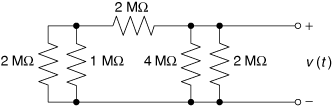
Find the lowest order lowpass Butterworth filter for which the difference between the 3 dB bandwidth and the noise bandwidth is less than 1%.
The RF amplifier for a certain receiver has a very simple two-pole bandpass filter with a 3 dB bandwidth of 2 MHz, centered at 10 MHz. The magnitude squared of the frequency response of the filter is
where f is the frequency in hertz. The input to the amplifier is white noise with power spectrum Si (f) = N0/2. Calculate the power spectrum at the output of the amplifier.
A certain receiver has a noise figure of 9 dB, a gain of 50 dB, and a bandwidth of 1 MHz. A resistive noise source in thermal equilibrium at 290 K feeds the input to the receiver.
A. Calculate the output noise contributed by the amplifier.
B. What is the total output-noise power in decibels above a milliwatt?
C. What is the equivalent total noise power referenced to the receiver input?
A receiver comprises four stages of amplification as follows:
Stage 1: 
Stage 2: 
Stage 3: 
Stage 4:= 
Noise at the receiver input comes from a source at noise temperature T0 = 290 K.
A. Compute the effective input-noise temperature of the receiver cascade.
B. Compute the noise figure of the receiver cascade.
C. If the last stage has a 1 MHz noise bandwidth, and the receiver sensitivity is 15 dB above thermal noise, what is the minimum detectable signal level in decibels above a milliwatt?
D. How does the minimum detectable signal change if the noise figure of the first stage is reduced to 2 dB?
For the system of Figure 2.30, assume that the IF amplifier has a 30 kHz bandwidth. Assume that the antenna noise temperature is 290 K and the receiver requires an SNR of at least 17 dB for reliable detection. What is the minimum required signal level?
Assume that the LNA in Figure 2.30 is moved to the antenna output terminals, just before the lossy transmission line. Under the conditions of Problem 2.16, what is the minimum required signal level? From the perspective of maximizing range, which arrangement is better and why?
A wireless link has the following parameters:
Effective isotropic radiated power, 
Path loss, 
System losses, 
Rx antenna gain, 
Rx noise bandwidth, BW = 100 KHz
Rx amplifier available gain, 
Rx noise figure, 
The noise temperature at the receiver antenna terminals is T0 = 290 K.
A.
B. A 300 ft feedline is added between the receiver's antenna and the amplifier input. The feedline has a loss of 1 dB/100 ft.
The uplink (mobile unit to base station) for an AMPS system has the following parameters:
Transmitter power, Pt = 3 W
Loss between Tx and antenna, 
Tx antenna gain, 
Rx antenna gain, 
Rx noise bandwidth, BW = 30 KHz
Rx noise figure, 
The noise temperature at the receiver antenna terminals is T0 = 290 K.
The base station uses two antennas to obtain a 3 dB received signal improvement called a diversity gain. This is included in the given value for Gr. Assuming a 6 dB margin and a 17 dB receiver sensitivity, what is the maximum range at which a mobile unit can be located to ensure good communications?