In the preceding chapter we developed the range equation assuming a free-space environment—that is, a perfect vacuum—with the nearest objects (other than the receiving antenna) being infinitely far away. Apart from applications such as communication between satellites, most wireless systems operate in a cluttered environment. We will refer to this environment as a "real-world" environment, since it represents the world in which we live. Unlike free space, a real-world environment includes an atmosphere through which radio waves must propagate and a variety of objects such as the Earth's surface, trees, and buildings.
The atmosphere and objects between and around the transmitter and receiver significantly affect a radio signal and may impair the overall system performance by attenuating or corrupting the signal. Objects in the propagation path may reflect, refract, and absorb some part of the signal. Signals may diffract around edges of buildings or other obstructions. Rough surfaces or groups of small reflecting surfaces such as the leaves on trees may scatter the signal in many directions. The Earth's surface can act as a reflector, producing a profound effect on path loss owing to destructive interference between a signal and its reflection. Over long propagation paths the atmosphere itself may absorb some of the electrical energy in a radio signal and dissipate that energy as heat. Variations in the density of the atmosphere may cause a signal to refract away from a preferred direction. The layered structure of the atmosphere may also cause a signal to be partially reflected.
Each of these real-world effects may be more or less significant depending on the specific application. For example, the effect of atmospheric absorption is much more troublesome for long-distance applications than for the shorter propagation distances normally associated with cellular telephone and personal communication applications. The varying density of the atmosphere allows radio waves to bend, leading to important applications in over-the-horizon communications and radar detection. Like atmospheric absorption, these refraction effects are of less importance for cellular telephone applications. For the applications that we will consider, atmospheric effects are negligible. This leaves reflection, diffraction, and scattering as the important short-distance real-world effects.
It is important to recognize that these real-world propagation effects are not entirely detrimental. In dense urban areas, and even in the downtown of a small city, buildings may obstruct the direct line-of-sight path between a mobile unit and any base station. In the absence of a direct propagation path to every location, one might expect that there would be many "shadowed" areas in which there would be no radio coverage. In practice, reflection, diffraction, and scattering "fill in the holes" and allow radio communication even when no direct path exists.
In the previous chapter we showed that the inevitable presence of noise in the receiver implies that a certain minimum power must be received to guarantee an acceptable quality of service. An important part of the design function performed by the systems engineer is to ensure that received signal power is adequate over the intended coverage area. In our development of the free-space range equation we showed that signal power decays with distance as d-2, where d is the free-space distance between the transmitter and receiver. The range equation thus provides a propagation model that can be used to predict received signal power, assuming, of course, that the propagation environment is adequately represented as free space. We will find, however, that in a real-world environment the free-space range equation is only a first step in modeling propagation between the transmitter and receiver. For example, when reflection from the surface of the Earth is taken into account, we find that the signal power may decay as d-4 rather than as d-2. Reflection, diffraction, and scattering caused by buildings and structures and by terrain features such as hills and ravines cause additional complexity in modeling propagation. It has been known for many years that at the carrier frequencies used for cellular and personal communication systems the received signal strength can vary significantly from point to point throughout the intended coverage area. These signal strength variations are so irregular, and so dependent on minute details of the physical environment, that it is practical to describe them only statistically. We will thus find that a systems engineer cannot as a practical matter guarantee adequate signal power over the entire coverage area. The best that can be done is to guarantee adequate signal power with high probability over a high fraction of the coverage area. Our aim in this chapter is to describe some of the phenomena that significantly alter signal propagation and to describe some of the models that can supplement the free-space range equation to enable systems engineers to design while taking these propagation effects into account.
Our chapter begins with an exploration of "macroscopic" or large-scale effects. We present a simple "two-ray" model that shows the consequences of reflection from the Earth's surface. A number of empirical models have been developed that relate average received signal power to propagation range, taking into account the heights of the transmitting and receiving antennas, the level of urban development, and features of the terrain. No single model has proved to be both simple enough to be usable and robust enough to be accurate under all circumstances. We will briefly describe the Okumura model and then present the Hata model and the Lee model in some detail. These models allow calculation of the median received signal power. Large-scale "shadowing" (including the effects of both reflection and diffraction) causes received signal strength to differ considerably from the median at different locations in the coverage area. We will introduce log-normal fading, a statistical model that gives a designer a basis for calculating the additional power needed to ensure a high probability of adequate coverage.
Next, the chapter moves on to "microscopic" or small-scale effects. The combination of reflection, diffraction, and scattering can cause multiple copies of the same signal to be received with different propagation delays. We again employ a simple two-ray model to show that this multipath reception can cause fading that, under certain circumstances, can be frequency selective. We follow our two-ray development with a more general model, the Rayleigh model, and introduce the concept of coherence bandwidth. The coherence bandwidth gives designers a basis for determining when frequency-selective fading will be an issue. Microscopic propagation effects also include fading caused by motion of a transmitter or receiver. We will find that this kind of fading is related to the Doppler spread of signals received over different propagation paths. We will once again demonstrate the effect by using a simple two-ray model, and then we introduce the concept of coherence time to provide a time reference for the speed with which fading occurs.
It is important to keep in mind that the motivation for developing the various propagation models is to give systems engineers the tools needed to design wireless systems that can meet quality of service objectives at an affordable cost. The chapter concludes with a continuation of the link analysis begun in Chapter 2 to show how a link budget can be developed that includes allowances for fading and coverage outages. In the subsequent chapter we will show how coverage can be extended to a large number of subscribers covering a virtually unlimited geographical area.
We observed in the introduction to this chapter that reflection from the surface of the Earth can significantly change the way in which received signal power depends on propagation range. We have several objectives in presenting a derivation of this effect. First, we will introduce the two-ray model, which we will use to good effect several times in this chapter. Next, reflection from the Earth's surface is one example of the reflection phenomenon; it illustrates what can happen when radio waves reflect from any surface. Finally, in showing how the variation of signal power with propagation range changes from d-2 in free space to d-4 above a reflecting Earth, we introduce the concept of path-loss exponent. We will show in a later discussion that signal power varies with propagation range as d-v in a real-world environment, where the path-loss exponent v typically takes values between 2 and 5.
Figure 3.1 is a representation of a uniform plane wave incident on the boundary between two different materials. In the most general case, some of the wave will be reflected from the boundary, and some of the wave will be transmitted. According to Snell's law, the angle of reflection from the boundary θr must equal the angle of incidence θi, where both angles are measured with respect to the normal to the boundary, as is shown in the figure. The angle of transmission into the second material θt will depend on the properties of the two materials. In general the incident, transmitted, and reflected signals will differ in amplitude and in phase, the relative amplitudes and phases depending on the properties of the materials and on the polarization of the incident wave. We will find it convenient to assume that the material labeled γ1 in the figure is air, whose properties for the purposes of the present discussion do not differ significantly from those of free space. If the material labeled γ2 in the figure is a perfect conductor, then there will be no transmitted signal, and the incident and reflected signals will have identical amplitudes. Alternatively, if the material γ2 is a perfect dielectric, then there can be both reflected and transmitted signals. In this case the amplitudes of the reflected and transmitted signals will depend on the dielectric properties of the two materials. The significant factor in this case is that there is no energy loss in the reflection, and all of the power in the incident wave will be either reflected or transmitted into the second material. In considering reflection from the Earth, we find that the second material, the Earth, cannot be taken as either a perfect conductor or a perfect dielectric. It turns out that the Earth is well modeled as a "good" conductor. This means that the amplitude of the reflected wave is nearly equal to the amplitude of the incident wave, particularly when the angle of incidence θi is near 90°. Nonetheless, some of the power in the incident wave will be transmitted into the Earth. The transmitted wave will be rapidly attenuated, however, and all of the power transmitted into the Earth is turned into heat.
Figure 3.1. Plane Wave Incident upon a Planar Boundary
Figure 3.2 shows transmitting and receiving antennas located above a conducting plane representing the Earth. For the propagation ranges commonly encountered in cellular and personal communication applications, it is reasonable to treat the Earth's surface as essentially flat. In the figure, the transmitting antenna represents a base station, and the receiving antenna a mobile unit, as might make up a typical cellular data link. The transmitting antenna is at height ht, the receiving antenna is at height hr, and the distance along the Earth from transmitter to receiver is d. The figure shows two rays extending from the transmitter to the receiver: a direct ray of path length Rdir and an indirect ray that reflects from the Earth and has path length Rind. Snell's law dictates that for the reflected ray ψr = ψi, a fact that can be used to find the location x of the reflection point. From the geometry of the figure, the length Rdir of the direct path is given by
Figure 3.2. Ground Reflections
For d >> ht + hr we can use a Taylor series to obtain a useful approximation:
The length of the indirect path is the sum of the path lengths of the incident and reflected parts. This length can be computed using straightforward geometry, but it is much simpler to recognize that the length of the indirect path can also be computed as the length of a path from the transmitting antenna to an "image" of the receiving antenna located hr below the surface of the Earth. Thus we have
Once again a Taylor series expansion gives the approximation
If the transmitted signal is a carrier wave of frequency fc, we can write the signal received over the direct path as

and the signal received over the indirect path as

In these expressions c is the speed of light and Φind is a phase change resulting from reflection from the Earth. Now the receiver obtains the sum of the signals specified by Equations (3.5) and (3.6), or
where the second line follows when we recognize that the sum of two sinusoids at a given frequency is another sinusoid at that same frequency. We are particularly interested in obtaining the amplitude A of the resulting sinusoid, as the average received signal power will be given by

Before combining the sinusoids, however, we observe that for reflection from a good conductor at a small grazing angle ψi, we have the approximation[1]

and

The simplest way of combining the sinusoids in Equation (3.7) is to express each sinusoid as a phasor and to add the phasors. If R is the phasor representing the total received signal, then
where we made use of Equations (3.9) and (3.10) in the second line, and in the third line we substituted the wavelength λ for c/fc. Next we make use of the identities
These give
The magnitude of the phasor R is the amplitude A that we seek. From Equation (3.13) we obtain

Observe that depending on the path length difference Rind - Rdir, the sine in Equation (3.14) can take any value between -1 and 1. When the sine takes the value 0, the direct and indirect rays arrive at the receiving antenna exactly out of phase and there is complete cancellation. When the sine takes the value ±1, the direct and indirect rays arrive exactly in phase, and there is complete reinforcement, leading to A = 2Adir.
To understand the consequences of Equation (3.14), let us make use of the approximations given in Equations (3.2) and (3.4). We find
so that Equation (3.14) becomes
Recall that sin θ ≈ θ for θ sufficiently small (for example, when θ = 0.5 radians the error is less than 5%). Then for  we may write
Substituting Equation (3.17) into Equation (3.8) gives
Now recall from Chapter 2 that for direct line-of-sight propagation the received signal power decreases as the square of the distance from the transmitter. In terms of amplitude, the value of Adir decreases as the distance, that is,

where the constant A0 may depend on transmitted power, antenna gains, and system losses, but not on distance. To be more explicit, if there were no reflection from the Earth, the received power would be given by
Using Equation (3.20), we can eliminate Adir from Equation (3.18):
Now the range equation tells us that for line-of-sight propagation over the direct path alone,
where we recognize that Rdir  d. Equating Equation (3.20) and Equation (3.22) gives us
Substituting Equation (3.23) into Equation (3.21) gives
Communications engineers would normally express Equation (3.24) in decibels, that is,

The factor of 4 in front of the 10 log (d) in Equation (3.25) is the so-called path-loss exponent.
The result we have obtained demonstrates the rather dramatic impact of placing a simple reflecting plane in the presence of a transmitter and receiver. Although the result is an approximation that assumes low grazing angles and a conductive Earth, it does represent a reasonable model for unobstructed terrestrial propagation. In the next section we will recognize that the real world places additional obstructions between the transmitter and receiver in wireless systems, and we will begin to consider more robust, but also more complex, propagation models.
Example
Suppose a wireless base station transmits 10 W to a receiver 10 km away over a flat, conductive Earth. The transmitting antenna has a gain of 6 dB, and the receiving antenna has a gain of 2 dB. The base station antenna is at the top of a 30 m tower, and the receiving antenna is on top of a pickup truck at an elevation of 2 m. The transmitting frequency is 850 MHz, and there are 2 dB of system losses.
Find the received signal power using Equation (3.25), and compare with the received power obtained from the range equation without considering reflection from the Earth. Evaluate the accuracy of the approximation made in getting from Equation (3.16) to Equation (3.17).
Solution
The transmitted power can be expressed in decibels as
Equation (3.25) gives
To compare with the result given by the range equation, we first calculate the wavelength as
The free-space path loss is then
The range equation gives
We see that ignoring reflection from the Earth gives an estimate of received power that is too optimistic by 13.4 dB (a factor of about 20).
To evaluate the approximation used to obtain Equation (3.17), we compute
Then
The approximation error is undetectable to three significant figures. Greater precision reveals an error of about 0.2%.
The purpose of macroscopic modeling is to provide a means for predicting path loss for a particular application environment. Any individual path-loss model has a limited range of applicability and will provide only an approximate characterization for a specific propagation environment. Nevertheless, modeling the communication path provides an extremely useful way to start a system design.
Modeling is useful for helping to understand how a proposed system will perform in a given environment, determining initial system layout, estimating the amount of equipment required to serve the application, and providing a means for predicting future expansion needs. The fact that predictions are only approximate, however, implies that results must be validated by measurement before financial investments are made to purchase equipment or obtain real estate. In the early days of cellular telephone development, base station equipment and purchase or lease of an antenna site could cost $1 million per cell. Clearly, confident predictions of how many cells are needed and their required locations and coverage areas can have a profound influence on the financial viability of a cellular system.
Although many models have been developed to cover the wide variety of environments encountered in wireless system design, we limit our discussion in this section to three outdoor models that are currently in use. These models are presented to demonstrate some of the current practice and to show how models can be used to perform radio system design in a real-world environment. All of the models we present are founded on the same set of underlying principles and the same approach to prediction. Although we present several models, our discussion is not meant to be a comprehensive treatment of all of the models available. To limit our discussion to a reasonable length we will not consider, for example, models that predict path loss in the indoor environment. These and other specialized outdoor models are well represented in the literature,[2] to which the reader is referred for further study.
The most widely used macroscopic propagation models are derived from measured data. Typically these models include the effects of terrain profile and some general characteristics of land use, such as whether the intended coverage area is urban or rural. In the previous section we found that a consequence of including reflection from the Earth in our propagation model was that the heights of the transmitting and receiving antennas became factors in determining the received signal power. The empirical models we will examine in this section also include the effects of antenna height, as well as the effects of carrier frequency. A typical formulation of an empirical model is to predict path loss based on measurements that use a specific reference system configuration, that is, a specific range of carrier frequencies, set of antenna heights, and terrain. Subsequently, correction factors are introduced to extrapolate the model to system configurations other than the reference configuration.
One of the most successful early attempts at providing a comprehensive model for the urban land mobile propagation environment was proposed by Okumura.[3] Using extensive measurements taken in Tokyo and the surrounding area, Okumura developed a set of curves that plot median signal attenuation relative to free space versus range for a specific system configuration. These curves span range values from 1 to 100 km and a frequency interval of 100 to 1920 MHz. Correction factors are provided to adjust the median path-loss value for differences in antenna height, diffraction, terrain profile, and land-use type. The Okumura model is entirely based on measured data and does not provide simple formulas for evaluation or extrapolation. Nevertheless, the Okumura model is considered simple to use and is widely employed for path-loss prediction in urban areas where it is most accurate. It is reported[4] to be accurate to around 10 dB to 14 dB compared with measurement.
The purely empirical nature of the Okumura model has made it difficult to incorporate into computer-based design tools. We will therefore focus our attention on two other models that are more analytic in nature and therefore more suitable for use in computer-aided analysis. These models are the Hata model and the Lee model.
The Hata[5] model is an analytical model that is based on Okumura's data. It produces path-loss predictions that compare favorably with those produced by Okumura's model. Because the Hata model provides formulas as approximations to Okumura's curves, it is well suited for computer implementation. The model is founded on a standard equation for the median path loss of a system in an urban environment. Median path loss means that for a given set of measurements, half of the data shows greater path loss than the median, and half less. The Hata model states
where the terms are as follows:
L50 (urban)|dB is the median path loss in decibels for an urban environment.
f0 is the carrier frequency in megahertz.
hte is the effective transmitting (base station) antenna height in meters.
hre is the effective receiving (mobile unit) antenna height in meters.
d is the range between transmitting and receiving antennas in kilometers.
a(hre) is a correction factor for mobile unit antenna height.
The mobile unit antenna height correction factor turns out to depend on the coverage area. For a large city it is given by
and for a small to medium-sized city it is given by

The Hata model contains additional correction factors for land use. In a suburban area

and in open and rural areas

The Hata model is applicable over the following range of parameters:
In all of these formulas, the logarithms are computed to the base 10. The "effective" antenna height is calculated by averaging the elevation of the terrain from 3 km to 15 km along the direction from the transmitting antenna to the receiving antenna. Antenna heights are measured as heights above this average.
The frequency range covered by the Hata model is not broad enough to include the PCS band at 1900 MHz. The European Cooperative for Scientific and Technical Research has proposed an extension to the Hata model that will extend its applicability to 2 GHz.
Example
A base station in a medium-sized city transmits from an antenna height of 30 m to a receiver 10 km away. The receiver antenna height is 2 m, and the carrier frequency is 850 MHz. Use the Hata model to determine the median path loss. Compare the median path loss with the path loss calculated using Equation (3.25) for propagation over a flat conductive Earth. How will the path loss predicted by the Hata model change if the receiving antenna is lowered to an effective height of 1 m?
Solution
For a medium-sized city, the mobile antenna correction factor is given by Equation (3.35), that is,
Then from Equation (3.33),
For comparison we take only the path-loss terms from Equation (3.25):
Note that in Equation (3.25) all distances are in meters. The Earth reflection model does not agree well with the Hata model in this instance. This suggests that the Earth reflection model is not sophisticated enough to be used for path-loss prediction in an urban environment.
In the Hata model only the correction factor a(hre) will change if the receiver antenna height is changed. For hre = 1 m,
This produces a median path loss of
Lowering the height of the receiving antenna increases the path loss by about 2.5 dB. Recall that 3 dB is a factor of 2, and that twice the path loss means that the receiver will receive half of the former signal power.
Example
The base station in the previous example transmits 10 W through an antenna of 6 dB gain. The receiver, at a height of 2 m, has an antenna gain of 2 dB. There are 3 dB of system losses. Using the results of the previous example, find the median received signal power.
Solution
The transmitter power in decibels is
Then the median received signal power is
The Lee model[6] is based upon extensive measurements made in the Philadelphia, Pennsylvania–Camden, New Jersey, area, and in Denville, Newark, and Whippany, New Jersey, by members of the Bell Laboratories technical staff in the early 1970s. Like the Hata model, the Lee model is widely used in computer-automated tools for radio frequency design of personal communication systems. Like the Okumura and Hata models, the Lee model provides a method for calculating path loss for a specified set of "standard" conditions and provides correction factors to adjust for conditions different from the standard.
The Lee model treats the area within one mile of the base station transmitter differently from the remainder of the coverage area. This is done for several reasons. First, proximity to the transmitter often ensures adequate signal strength. Next, there is a high probability that propagation to a receiver near the base station will be line-of-sight. Finally, a receiver near the base of the transmitting tower may be below the main beam of the transmitting antenna, causing the antenna gain to be lower than normal. The reference distance of one mile is a somewhat arbitrary standard, but it ensures that the influence of the environment near the transmitting antenna does not significantly bias the path-loss prediction over the entire coverage area.
Example
As a preliminary to introducing the actual Lee model, consider a system for which line-of-sight conditions hold out to a reference range of d0, after which there is a path-loss exponent of value ν. Let us evaluate the received signal power at a range d > d0.
The free-space range equation gives us, assuming free-space conditions out to range d,
If we replace the path-loss exponent of 2 with ν for propagation from d0 to d, then Equation (3.45) becomes
Let us define a "reference" received power Pr0 as the received power at distance d0. Then Equation (3.46) becomes

Converting to decibels, we can write
The Lee model follows the form of Equation (3.48) using a reference distance d0 of one mile. The reference power  and the path-loss exponent have been determined from measurements. The Lee model initially assumes a standard set of reference conditions and a flat terrain. Correction factors are added to account for differences from the reference conditions and to allow the path loss to be corrected on a point-by-point basis for the specific terrain profile. The standard conditions for the Lee model are as follows:
 .
. with respect to the gain of a half-wave dipole (8.15 dB with respect to an isotropic radiator). with respect to the gain of a dipole antenna (that is, 2.15 dB with respect to an isotropic antenna).
The Lee model has been shown to be applicable for frequencies up to 2 GHz. It is most often expressed in terms of the median received power level as
where
 is the median received power level in decibels above a milliwatt
 is the median received power level at the one-mile reference range in decibels above a milliwatt
v is the path-loss exponent for the specific type of area
d is the total range between the transmitter and receiver antennas
d0 is the reference range of one mile
αc is the correction factor in decibels for system parameters different from the standard
The correction factor αc provides a means for converting median received power level from a prediction based on standard parameters to a prediction based on actual parameters. The correction factor is given by
where the parameters  and
and  are the actual system parameters, and the parameter n is given by
The correction factors for antenna height are consistent with Equation (3.25). The Lee model assumes that the mobile receiver's antenna height is not greater than 10 feet. The model may also include a correction term for diffraction that applies when the propagation path is blocked by an obstruction such as a hill.
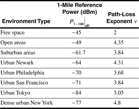
Based on measurements, Lee provides values for the one-mile reference power and the path-loss exponent for various types of environment. These values are given in Table 3.1.
Table 3.1. Measured Reference Power and Path-Loss Exponent for Various Environments
Lee's model as given by Equation (3.49) can be further corrected to include the effect of terrain that is not flat.[7] The additional correction factor is
where heff is an "effective" base station antenna height computed as shown in Figure 3.3. The two configurations shown in the figure are characterized by the property that the radio waves reflect from a slope rather than from a horizontal surface. In practice, terrain profiles can be determined using geographical databases that provide elevation versus geographic coordinates for the intended coverage area. Such databases are readily available for commercial applications in most areas worldwide. An array of "bins" can be defined along a radial line from the base station antenna. The average elevation and slope of each bin are taken as the elevation and slope at the center of the bin. An effective transmitter antenna height can then be calculated for the center of each bin. Once effective antenna height is determined, Equation (3.49) corrected by Equation (3.52) will give a prediction of median received signal power. Thus the local terrain profile can be used to modify the signal strength prediction.
Figure 3.3. Computing the Effective Base Station Antenna Height: (a) Mobile Antenna on a Slope; (b) Base Station Antenna on a Slope
Example
A base station in a medium-sized city transmits 43 dBm from an antenna height of 30 m to a receiver 10 km away over flat terrain. The receiver antenna height is 2 m, and the carrier frequency is 850 MHz. The base station antenna has a gain of 10 dBi, and the mobile unit antenna has a gain of 2 dBi. Use the Lee model to determine the median received signal power.
Compare the median received signal power with that obtained using the Hata model.
Solution
If we take urban Newark as a "medium-sized city" (compared to Philadelphia, Tokyo, or New York), then  and v = 4.31. Now 10 km is about 6.2 miles. Then
Equation (3.49) gives
To determine the correction factor, we observe that our 30 m base station antenna height is close to the 100 ft standard, and the 850 MHz carrier frequency also corresponds to the standard. The 2 m mobile unit antenna height is about 6.56 ft. We therefore have
As there is no correction needed for terrain, we obtain

To compare with the Hata model, we begin with the path loss obtained in Equation (3.39), L50 (urban)|dB= 160 dB. Then
The Lee and Hata models differ in their predictions by about 8 dB. Neither model is in error; the difference represents the limited accuracy that can be obtained from simple models of real-world propagation. Clearly systems engineers must apply considerable engineering judgment based on experience and backed by field measurements before investing money based on the predictions of these models. The fact that cellular telephone systems work as well as they do is testimony to the fact that engineers are in fact able to apply the necessary judgment and use the models to produce successful designs.
In the previous section we investigated a number of models that allow a systems engineer to predict median path loss as a function of the distance between transmitting and receiving antennas. The models also relate path loss to various system parameters such as antenna height and carrier frequency. The fact that these models predict median rather than absolute path loss suggests that measurements made at various locations at a given separation distance will produce a range of path-loss values. If we wish to design a communication system that will provide an acceptable quality of service not just "on the average" but at most locations in the coverage area, we will have to extend our path-loss models to enable us to predict not just median loss, but also the range of loss values we are likely to encounter at a given distance from the transmitter. One reason for the change in path loss with location at a given separation distance is that shadowing from various obstructions distributed over the signal path changes as the transmitter or receiver position is varied. It has been found that path-loss changes caused by shadowing are relatively gradual. This means that location must change by many wavelengths before a significant change in path loss will be observed. Another phenomenon, multipath propagation, is responsible for significant path-loss changes over distances of less than a wavelength. We will investigate these "microscopic" propagation effects in a later section of the current chapter.
In principle it should be possible to calculate the path loss for every location in the environment at a given distance between the transmitter and receiver. All that is needed is a detailed enough description of the physical environment between, and in the vicinity of, the transmitter and receiver, and powerful enough electromagnetics modeling software. In practice, of course, the detailed description of the environment is not available, and the calculations would be complicated. Consequently we will use a statistical model to account for the gradual variations in path loss produced by shadowing. In this model we will let the path loss  be modeled as a random variable. If the mean of this random variable is
  , then we can write
where the term  is a random variable with zero mean. The mean path loss is reasonably well predicted by the median path loss obtained from the Okumura, Hata, or Lee model. It remains for us to characterize the random part of the path loss. Extensive measurements for a wide variety of environments have consistently demonstrated that the path loss, when expressed in decibels, follows a normal, or Gaussian, distribution. The probability density function fl(ξ) for is therefore
where σpath is the standard deviation of the random variable . We say that the path loss , or equivalently its random part , follows a log-normal distribution, where the logarithm comes from the fact that path loss is expressed in decibels. Note that the received signal power at a given separation distance can be written
where  is the average received signal power at the given distance. Thus
  is also a log-normally distributed random variable with the probability density function fp(ρ) given by
Using the probability density function of Equation (3.60), we can express the probability that the received signal power is less than or equal to a given value as
Similarly, the probability that the received signal power is greater than is
The standard deviation σpath is a parameter that must be chosen to calibrate the statistical model for a given environment. Measurements and empirical studies of extensive data reveal that the standard deviation of the log-normal distribution is approximately 8 dB for a wide range of urban and suburban environments. The standard deviation may be 1–2 dB higher for dense urban environments and 1–2 dB lower for open and rural areas.
The integrals encountered in Equations (3.61) and (3.62) cannot be evaluated in closed form. Owing to the importance of these integrals in a variety of statistical applications, however, they are widely tabulated. Usually tables provide standardized versions of these probability integrals. One standardized form, the Q-function, is defined as
In terms of the Q-function, Equation (3.62) becomes
The Q-function has the useful property that
This allows Equation (3.61) to be expressed as
There is a table of Q-function values in Appendix A. Appendix A also presents an alternative standard form, the error function. The error function is tabulated in numerous mathematical tables and can also be evaluated using software applications such as MATLAB.
Example
A cellular base station transmits 20 W at 850 MHz from an antenna with 4 dBi of gain at a height of 40 m. A mobile receiver has an antenna gain of 0 dBi at a height of 1.5 m. There are 2 dB of system losses. The mobile unit is located at the perimeter of the cell, at a distance of 8 km from the transmitting antenna. The cell is in the suburbs of a small city.
Use the Hata model to find the median received signal power. Then find the probability that the received signal power will actually be 10 dB or more below the median. The standard deviation of received power is 8 dB.
Solution
Beginning with Equation (3.35), the correction factor for a small city is α (hre) = 0.0136 dB. Then Equation (3.33) gives L50(urban)|dB= 145 dB. Using Equation (3.36) to correct for land use, we obtain L50(suburban)|dB= 145 dB. Now we can use the median path loss to obtain the median received signal power:
We will take this median received signal power as the average received signal power in our log-normal statistical model, that is,

Now we wish to find  . Using Equation (3.66) with σpath = 8 dB,
using the Q-function table in Appendix A.
It is important to interpret the result given in Equation (3.69) correctly. The signal strength at any location near the cell boundary, whatever that strength happens to be, will not change, so long as the receiver and the surrounding environment remain motionless. If signal strength is measured at a number of locations near the cell boundary, however, the received signal power will be at or below -110 dB at about 10% of the locations. Our model tells us nothing about how far the receiver must be moved to go from a location with signal power above -110 dB to a location with power below -110 dB.
Example
A base station in a cellular system transmits at 890 MHz from an antenna of gain 6 dBi at a height of 35 m to a mobile unit with an antenna gain of 2 dBi at a height of 2 m. There are 1.5 dB of system losses. The cell is located in a large city. The mobile unit is at the edge of the cell, at a distance of 2 km from the base station. Suppose the receiver in the mobile unit requires a signal power of -90 dBm to provide the subscriber with an adequate quality of service (that is, the receiver sensitivity is -90 dBm). If σpath = 9 dB, determine how much power the base station must transmit so that the received power will be adequate at 80% of locations at the cell limit.
Solution
We want to guarantee that  . Now Equation (3.64) gives us
Using Equation (3.65), this becomes
From the Q-function table in Appendix A we find
Solving gives the average receiver power needed at the cell limit:
If we take the average receiver power as equivalent to the median power predicted, say, by the Hata model, we can write

Using the Hata model, we find that  , so that Equation (3.74) gives the required transmitter power,
  .
.
The difference between the average received signal power and the receiver sensitivity is called the fade margin. In this example a fade margin of 7.6 dB was needed to ensure adequate received power at 80% of locations 2 km from the transmitter.
In the previous section we developed a model to account for the variation of path loss with location, given a constant separation distance between the transmitting and receiving antennas. The primary physical phenomenon that was reflected in this model is shadowing by objects in the environment between the transmitter and receiver. The effect of shadowing is sometimes called macroscopic or macro-scale fading, or sometimes large-scale fading, as shadowing causes received signal strength to change as the receiver moves over distances that are long compared with a wavelength. The term log-normal fading is also used to describe this phenomenon, because the received signal power can be accurately modeled as a random variable with a log-normal probability distribution. In the current section we begin our examination of a different fading phenomenon. This fading is caused by multipath propagation, that is, reception of the same signal over two or more propagation paths. Multipath propagation causes the received signal power to change significantly as the receiver is moved over distances shorter than a wavelength and is consequently referred to as microscopic or small-scale fading.
Multipath propagation arises because of the presence of objects in the environment that can reflect or scatter the transmitted signal. Figure 3.4 suggests copies of a transmitted signal arriving at a receiver by multiple paths. Buildings and other man-made structures, hillsides, and the leaves of trees are examples of potential scatterers. In urban environments there may be many such scatterers, and copies of the transmitted signal may arrive at the receiver by a large number of simultaneous paths. When a signal reflects from a scattering surface, it may undergo a change in amplitude and a change in phase. Signals arriving at the receiver over multiple paths will then include these amplitude and phase changes. Further, each path will in general have a different length, so the received signals will arrive with slightly different delays. If the transmitter, the receiver, or any of the scatterers is in motion, signals will arrive at the receiver with a spread of Doppler shifts. This Doppler spread can cause the received signal strength to vary with time, even if the receiver's position does not change.
Figure 3.4. Multipath Propagation Caused by Reflection from Multiple Objects
We will begin our study of micro-scale fading by considering a two-ray propagation model. This model, though simple, will allow us to discover and begin to quantify a number of important attributes of multipath propagation. The two-ray model will illustrate how constructive and destructive interference causes the received signal strength to be a function of receiver position. The simple model will also illustrate that the path loss of a multipath communication channel is frequency dependent, even when the receiver's location is fixed. This frequency dependence adds a new wrinkle to our propagation model. In some cases the loss is relatively constant over the bandwidth used by a single transmitter and receiver. In other cases the loss will vary within this bandwidth, leading to distortion of the received signal. We will find that the band of frequencies over which the loss remains approximately constant is dependent on the difference in delay times between the two arriving signals.
Once we have used the two-ray model to demonstrate the underlying causes of small-scale fading and frequency-dependent path loss, we will introduce a statistical model for the real-world case in which there are many received signals. The statistical model is called the Rayleigh model, after the probability distribution that plays a significant role in characterizing the amplitude of the received signal. The Rayleigh model will allow us to calculate the probability of a fade, much as the log-normal model allowed us to make that calculation for shadowing. To design a data link that will provide users with a high quality of service, allowance must be made for both macroscopic and microscopic fading. The statistical model will also give us a framework for defining a root-mean-square (RMS) delay spread, which we will use to obtain a quantitative estimate of the coherence bandwidth, that is, the bandwidth over which the loss remains approximately constant.
After establishing the Rayleigh model and frequency-dependent loss, we shall return to the two-ray model for insight into the case in which the receiver is in motion. We will be able to easily show how motion of the receiver produces a time-varying path loss. We will be able to characterize the timescale over which the loss varies in terms of the Doppler shifts in the carrier frequencies of the two received signals. The statistical model, which we will not treat in detail, yields a coherence time, defined as the time over which the path loss remains approximately constant. We will use the coherence time as a boundary between the cases of "slow" fading, in which the path loss remains nearly constant during the time required to receive a single pulse, and "fast" fading, in which the path loss changes while the pulse is in flight.
Figure 3.5 shows a single transmitted signal traveling to a receiver over two propagation paths. To keep the model simple, we will assume that the transmitted signal is an unmodulated carrier. In practice, of course, the carrier will be modulated in some way with an information signal. One effect of modulation will be to give the transmitted signal a nonzero bandwidth. Although we do not show the modulation explicitly in the discussion to follow, we recognize that the transmitted signal's bandwidth makes the frequency response of the multipath channel a matter of concern.
Figure 3.5. A Signal Received over Two Propagation Paths
The received signal can be written

where
A1 and Φ1 are respectively the amplitude and phase of the signal received over path 1
A2 and Φ2 are the amplitude and phase of the signal received over path 2
t1 is the propagation delay corresponding to path 1
t2 is the propagation delay corresponding to path 2
f is the frequency
Following our approach in Equation (3.7), we will write the received signal as a single sinusoid:
We are particularly interested in the amplitude A of this combined received signal. Using phasors to combine the two sinusoids in Equation (3.75), we obtain

The magnitude of the resultant phasor R is a little easier to find if we factor out the first term. This gives
Expanding the exponential in the parentheses using Euler's identity and combining real parts and imaginary parts gives
Now we can compute the magnitude as the square root of the square of the real part plus the square of the imaginary part:
where we have simplified by combining cosine-squared and sine-squared terms. This result shows that the amplitude A of the received signal depends on the phase difference Φ2 - Φ1, on the delay difference t2 - t1, and, most interestingly, on the frequency f.
The amplitude of the combined signal given by Equation (3.80) can be larger or smaller than the amplitude of the signal received over either single path. If, for example, Φ2 - Φ1 = 0, and the path lengths differ by an integral number of wavelengths (that is, an even number of half-wavelengths), then the signals received over the two paths will combine constructively. In Equation (3.80) the cosine will take the value +1, giving A = A1 + A2. Alternatively, if Φ2 - Φ1 = 0 and the path lengths differ by an odd number of half-wavelengths, then the signals received over the two paths will combine destructively. In Equation (3.80) the cosine will take the value -1, and the amplitude of the combined signal will be A = |A1 - A2|. In general, the amplitude of the combined signal will take a value between these extremes. The amplitude of the received signal is not a function of time; this amplitude will remain constant as long as all of the parameters in Equation (3.80) remain constant. If the position of the receiver is changed, however, then the delay difference t2 - t1 will change, causing a change in the amplitude A. In an extreme case, with the two signals arriving from opposite directions, a change in receiver position of only a quarter-wavelength could cause one path to become a quarter-wavelength longer and the other path to become a quarter-wavelength shorter. The net effect could change the received signal strength from a maximum associated with constructive reinforcement to a minimum associated with destructive cancellation. This change in received signal strength with small changes in receiver position is often referred to as small-scale fading, since the distances over which the receiver must move to cause or end a fade are small compared with the wavelength. (At 850 MHz a wavelength is only 0.35 m.) It is important to note that the number of wavelengths by which paths 1 and 2 differ depends on the frequency f. This means that a small change in frequency can also result in a significant change in the amplitude of the combined received signal.
Example
Suppose the phase difference Φ2 - Φ1 is π/3, the amplitude difference is 2 dB, and path 2 is 150 m longer than path 1. Plot the received signal amplitude versus frequency, for frequencies from 850 to 855 MHz.
Solution
Let us suppose that path 1 produces the stronger signal. Then the 2 dB amplitude difference means that  , so A2/A1 = 0.794. The delay difference t2 - t1 is given by
  . Equation (3.80) now gives

Figure 3.6 shows A/A1 plotted against frequency. This figure is called a "standing wave pattern" in the electromagnetics literature. At 850.3 MHz the 0.5 μs difference in the propagation delays of the two paths represents an integral number of wavelengths, and the signals reinforce. At 851.3 MHz this same time difference corresponds to an odd number of half-wavelengths, and the signals partially cancel. We note that the ratio of maximum amplitude to minimum amplitude is  .
.
Figure 3.6. Received Signal Relative Amplitude versus Frequency
In Figure 3.6 the relative amplitude is periodic in frequency with a period of 2 MHz. This means that a transmitted signal with a bandwidth much less than 2 MHz will propagate over a communication channel whose path loss is relatively constant over the signal bandwidth. A transmitted signal with a bandwidth comparable to 2 MHz, on the other hand, will experience a communication channel whose path loss varies significantly with frequency. The former case is referred to as "flat fading" and the latter case as "frequency-selective fading."
Example
Plot the relative amplitude described in Equation (3.81) over two 30 kHz frequency bands, one centered at 851.5 MHz and one centered at 852.5 MHz.
Solution
The required plots are shown in Figure 3.7. These graphs depict flat fading over two 30 kHz wide "channels." They show that in the given example, the received signal amplitude varies very little with frequency over a 30 kHz band, although the amplitudes are significantly different at the two carrier frequencies spaced 1 MHz apart.
Figure 3.7. Flat Fading: Received Signal Relative Amplitude versus Frequency for 30 kHz Channels at Two Carrier Frequencies
In the example shown, the received signal amplitude varies with frequency in a periodic manner, with spectral nulls (fades) occurring every 2 MHz. Referring to Equation (3.80), we can see that in the general case the amplitude level will repeat whenever the frequency changes over an interval that causes the argument of the cosine to change by 2π radians. If fn - n represents the null-to-null frequency interval, then
or
We see that the null-to-null interval is inversely proportional to the "delay spread" t2 - t1. A modulated signal will experience flat fading if the signal bandwidth is much less than the reciprocal of the delay spread. Conversely, a modulated signal will experience frequency-selective fading if the signal bandwidth is comparable to or greater than the reciprocal of the delay spread.
It is common in dense urban environments for there to be no direct line-of-sight path from a transmitter to a receiver. In this case communication is made possible only by reflection and refraction from objects in the environment, particularly buildings. We will assume in what follows that the received signal is the sum of a large number M of waves all originating from the same transmitter, but all arriving from different directions, and each with its own amplitude, phase, and delay. Thus the received signal is
where the angle θk is given by

Following our usual procedure, we use phasors to add the sinusoids in Equation (3.84),
where  , and
, and  .
.
In a real-world environment we cannot measure the specific properties of all of the individual propagation paths that produce components of the received signal. We will therefore characterize the received signal statistically by representing Ak, k = 1, ..., M and θk, k = 1, ..., M as random variables. A few reasonable assumptions will greatly simplify our characterization.
These assumptions, together with the additional assumption that the number of signal components M is large, allow us to invoke the central limit theorem and consequently to assert that the random variables X and Y defined in Equation (3.86) are statistically independent Gaussian random variables, with zero means and equal variances σ2. The Gaussian model correlates well with measured data taken in representative environments.
The joint probability density function fX, Y (x, y) of X and Y is the familiar "bell curve," which can be written as
The cumulative probability distribution function FX, Y (x, y) is, for any real numbers x and y, the joint probability that X ≤ x and Y ≤ y, that is,
A little calculus reveals that
As in the two-ray model, we are interested in the amplitude A of the total received signal r (t). Recall that A is the magnitude of the phasor R, defined in Equation (3.86), that is,
The amplitude A is a random variable, which means that we need to find its probability density function fA (a) rather than its value. Our approach will be to first find the cumulative probability distribution function FA (a) and then take the derivative as in Equation (3.89) (a single derivative in this case) to find fA (a). Now the phasor R can be written in polar form as

where A is given by Equation (3.90) and

Using the dummy variables ξ, η, α, and θ, Equations (3.90) and (3.92) become

We wish to find

The region of integration is shown in Figure 3.8. Using Equation (3.93) to transform to polar coordinates gives us ξ2 + η2 = α2 and the area element dξdη = αdθdα.
Figure 3.8. Region of Integration for Cumulative Distribution Function of Received Signal Amplitude
Substituting in Equation (3.94) gives
Finally,
The probability density function fA(a) for the amplitude of the received signal is known as a Rayleigh density function. It has a mean value mA given by

and a standard deviation σA given by

Note that the standard deviation of the Rayleigh distribution is σA, given by Equation (3.98), and is not the parameter σ. A Rayleigh probability density function is illustrated in Figure 3.9 with σ = 1.
Figure 3.9. A Rayleigh Probability Density Function with σ = 1
Figure 3.10 shows 100 samples of a Rayleigh-distributed random variable plotted in decibels. The horizontal axis is the sample number and does not represent time or position. This figure shows values of received signal amplitude that might be obtained from measurements taken in a multipath environment at positions a few wavelengths apart. The mean of the received signal amplitude has been set at zero decibels. Notice that a few of the samples show very deep fades.
Figure 3.10. One Hundred Samples of a Rayleigh-Distributed Random Variable
Now that we have characterized the statistical behavior of the received signal amplitude, we can turn our attention to the received signal power. Average received power is related to amplitude by Equation (3.8), repeated here for convenience:

Since the amplitude A is modeled as a random variable in the current analysis, so is the power Pr. We must then determine the probability density function for Pr. As we did for amplitude, we begin by seeking the cumulative probability distribution function FP(p) = Pr{Pr ≤ p}. Now Equation (3.99) shows that Pr ≤ p whenever  (recall that A cannot be negative).
We then have
Following our customary practice, we obtain the probability distribution function for power by differentiating Equation (3.100):
The received signal power Pr is said to have an exponential probability distribution. The mean mP and standard deviation σP are equal and are given by

Example
A signal in a multipath environment is received with an average power of -100 dBm, where the average is based on a number of samples taken in a local area. Find the probability that an additional sample will measure no more than -110 dBm.
Solution
Since the samples are taken in a local area, we assume that the variation in measured power between samples is not attributable to changing distance from the transmitter or changes in shadowing. We therefore assume a Rayleigh model. Now -100 dBm is a power of 100 x 10-15 W. Using Equation (3.102), we have
Similarly, -110 dBm is a power of 10 x 10-15 W. We can write, using Equation (3.101),
Example
A mobile receiver in a wireless system has a sensitivity of -95 dBm. As the receiver is moved in a local area, we wish to provide an 85% probability that the received signal will remain above the receiver sensitivity. What average received signal level is required?
Solution
First we recognize that -95 dBm is 316 x 10-15 W. Next, using Equation (3.101),
Solving for σ2 gives σ2 = 1.95 x 10⁻¹² W. According to Equation (3.102), this is the average received signal power. Converting to decibels gives the answer as -87.1 dBm.
When one of the many signals that contribute to Equation (3.84) is much stronger than the others, the resulting composite signal can be modeled by a random variable having a Ricean probability distribution. This situation can occur, for example, when there is a direct line-of-sight path between the transmitting and receiving antennas in addition to multiple paths that involve scattering by reflection or diffraction. The Ricean distribution is named after S. O. Rice, who, in a classic paper,[8] used it to characterize a signal composed of a DC component plus thermal noise. The presence of a strong line-of-sight component implies that one of the components of Equation (3.86) will have a nonzero mean value. If we take the component with the nonzero mean as X, then Equation (3.87) must be modified to read
Following the steps in Equations (3.94) through (3.96) gives
where I0(η) is the zeroth-order modified Bessel function and is defined as the integral
Bessel functions can be evaluated using mathematical tables or software applications such as MATLAB or Maple.
It is convenient to describe the ratio of power in the line-of-sight component of a signal  to the power in the scattering components of the signal σ2. Specifically, we define
Figure 3.11 is a plot of the Ricean probability density function for several values of  . Note that when the level of the line-of-sight wave is small (i.e.,
  ), the density function approaches a Rayleigh density. As the line-of-sight component becomes large compared to the scattering components, the density function tends toward a Gaussian shape.
Figure 3.11. Ricean Probability Density Functions
When a large line-of-sight component is present in a received signal, the effects of small-scale fading are reduced. This is because the peaks and nulls caused by constructive and destructive interference are less significant in relation to the average or steady component of the signal.
We learned from the two-ray model that in a multipath environment, fading is not only a consequence of changes in receiver position but is also caused by changes in frequency. We found that the frequency interval over which the received signal level remains approximately constant is inversely proportional to the delay spread, which in the two-ray model was t2 - t1. In the general multipath case there are many copies of the received signal arriving over different paths, each with a different delay. Figure 3.12 shows a typical standing wave pattern in which received signal amplitude is plotted versus frequency. The graph shows the same general effect as does Figure 3.6: There are frequencies at which the received signal components tend to add constructively, giving a large received amplitude; and there are frequencies at which the received signal components add destructively, leading to a small received amplitude. The plot of Figure 3.12 is more irregular than the two-ray result plotted in Figure 3.6. With reference to the standing wave pattern of Figure 3.12, we can define the coherence bandwidth Bcoh as the frequency interval over which the received signal amplitude is relatively constant. The literature contains several definitions of coherence bandwidth, the difference depending on exactly what is meant by "relatively constant" signal amplitude. To get a quantitative sense of coherence bandwidth, we must examine the concept of delay spread a little more closely.
Figure 3.12. Received Signal Relative Amplitude versus Frequency for a Multipath Channel
Suppose the transmitted signal is an impulse. If there were a single path from transmitter to receiver, the received signal would also be an impulse, attenuated and arriving after a delay. In a multipath environment the total received signal will be a scattering of impulses, each arriving with a delay particular to the propagation path it traversed. Figure 3.13 shows a train of impulses having power levels p1,..., pM and arriving at times t1,...,tM respectively. In the figure, M = 5, and the plot is called the "power delay spread" function of the multipath communication channel. With reference to Figure 3.13, we can define the mean delay as
Figure 3.13. Power Delay Spread Function of a Multipath Communication Channel
Notice that this is a weighted average, so that the strongest impulses have the greatest influence in determining the value of the mean delay. For the purpose of computing this average and the one to follow, powers are not expressed in decibels. The mean square delay is defined to be

Note that in Equation (3.111) the delay times are squared but the powers are not. Using Equation (3.110) and Equation (3.111) to define the RMS delay spread σd, we obtain
The RMS delay spread is a measure of the spread centered on the mean delay  . Absolute delay values turn out not to be relevant.
When the total number M of received components is large, it is convenient to model the power delay spread function of Figure 3.12 as a continuous function. We will represent this function by p (t), where p (t) has been normalized (by dividing by  ) so that
  . There is some experimental evidence to show that a good model for p (t) is exponential, that is,
To formally treat the concept of "coherence,"[9] we consider the received signal at two neighboring frequencies f1 and f2. (We can arbitrarily choose f2 to be the larger frequency.) The corresponding phasors R1 and R2 are each given by an equation like Equation (3.86). Now Equation (3.86) contains the angles θk, which depend on frequency and on path delay through Equation (3.85). The real and imaginary components X1, Y1, X2, and Y2 of the phasors R1 and R2 are four jointly Gaussian random variables. The joint probability density function for these random variables can be written out once the variances and covariances of the random variables are known. It turns out that all of the necessary variances and covariances can be obtained from Equation (3.86) by averaging over the time delays using Equation (3.113). Once we have a joint probability density function for X1, Y1, X2, and Y2, we can transform to polar coordinates as we did in developing Equation (3.96). The result is a joint probability density function for the received signal amplitudes A1 at frequency f1 and A2 at frequency f2. Finally, this joint density function can be used to calculate the correlation coefficient ρ between A1 and A2. The math is a little bit tricky, but the resulting correlation coefficient is
We can see from Equation (3.114) that the amplitudes of the signals at frequencies f1 and f2 will be highly correlated if f2 - f1 is small. The signal amplitudes will become less correlated as the frequencies move apart. Now we can define the coherence bandwidth as the frequency interval f2 - f1 for which the correlation coefficient ρ is at least 0.5. Solving Equation (3.114) with ρ = 0.5 gives  . Writing Bcoh in place of f2 - f1, the coherence bandwidth is usually rounded off and written as

To appreciate the importance of coherence bandwidth, it is important to remember that the received signal is not a pure carrier (or an impulse) but a modulated carrier. As such the received signal will have some bandwidth of its own, Bsig. When Bsig << Bcoh we have flat fading. Although the received signal level may be enhanced by constructive interference or reduced by destructive interference, the signal level will remain nearly constant over the bandwidth Bsig. Alternatively, when Bsig >> Bcoh, we have frequency-selective fading. The signal level changes within the band Bsig, distorting the received signal.
It is interesting to compare the effects of flat and frequency-selective fading in the time domain. If the transmitted signals are digital, the duration of a pulse Tsig will be roughly  , give or take a factor of 2. Now for flat fading,
This means that the M copies of the received pulse all arrive within a time span that is short compared with the duration of a single pulse. As a result, when the M pulses are added at the receiver input, there is little distortion of the pulse shape. Now the time spread σd is short compared with the pulse duration, but it may not be short compared with the period of the carrier. Thus copies of the received pulse may arrive with carrier phases spanning all possible angles. The carriers may add constructively or destructively. This gives flat fading its characteristic property: There is little distortion to the shape of the received pulse, but its amplitude may be enhanced or decreased. For frequency-selective fading we have the opposite effect:
In this case the received pulses are spread over a long enough time span that individual pulses can be resolved at the receiver. This means that when the transmitter produces a continuous train of pulses, each pulse will be spread by the multipath propagation so that there is intersymbol interference at the receiver. A multipath channel with a large RMS delay spread is sometimes described as time dispersive. Intersymbol interference must be dealt with at the receiver much as it is dealt with in a telephone modem. An equalization filter is used to flatten the channel frequency response and thereby undo the effect of the frequency-selective fading. Since the way the received signal level varies as a function of frequency will change when the receiver is moved, the equalizing filter must be adaptive. Adaptive equalization is usually implemented with digital signal processors. Design of adaptive equalizers is a fascinating topic that space does not allow us to treat in this text. We will, however, revisit this topic when we examine the ability of spread-spectrum modulation systems to give good performance in frequency-selective fading conditions.
Figure 3.14 shows pulses received over a simulated multipath channel. The RMS delay spread in the simulation was set to σd = 0.5 μs. The left-hand column shows pulses having a width of about Tsig = 3.33 μs. Since Tsig >> σd, this case represents flat fading. Notice that the three pulses shown all have nearly the same shape but different amplitudes. The right-hand column shows pulses having a width of about Tsig = 0.33 μs. This case shows frequency-selective fading. Observe that individual pulses that arrive over different paths can be resolved.
Figure 3.14. Flat and Frequency-Selective Fading in the Time Domain; the RMS Delay Spread Is 0.5 μs
Example
Figure 3.15 shows the power delay spread for a particular multipath channel. The transmitter and receiver are both stationary. In the figure, the relative powers of the received impulses are  ,
,  ,
,  , and
, and
 . The corresponding arrival times are t1 = 2 μs, t2 = 2.8 μs, t3 = 3 μs, and t4 = 5 μs. Determine the RMS delay spread and the coherence bandwidth. If a communication signal using this channel has a bandwidth of Bsig = 30 kHz, will the signal experience flat fading or frequency-selective fading?
Figure 3.15. A Power Delay Spread Function
Solution
First we must convert the relative powers out of decibels. We obtain p1 = 1, p2 = 0.794, p3 = 1.141, and p4 = 1. Next we use Equation (3.110) to obtain the mean delay time:
Then we use Equation (3.111) to calculate the mean-square delay,
and Equation (3.112) to give the RMS delay spread,
Now the coherence bandwidth is given by Equation (3.115):
Finally, for a communication signal with Bsig = 30 kHz, we have Bsig << Bcoh, so the fading will be flat.
In a real-world communication environment it is unusual for the mobile radio to remain motionless. People using cellular telephones commonly walk or ride in vehicles while talking on the phone. If the mobile unit is in motion during communications, the mobile antenna travels through the standing wave pattern caused by multipath propagation. The effect is the same whether the mobile unit is receiving or transmitting: The received signal level at the mobile unit or at the base station fluctuates as the location of the mobile unit's antenna changes. This is our first encounter with a time-varying communication channel. We are concerned with the rate at which the received signal level varies. If the signal level changes slowly with respect to the time that it takes to receive a single pulse, then individual pulses will not be distorted. If the received signal level remains above the receiver's sensitivity, an acceptable quality of service can be maintained regardless of the time-varying fades. On the other hand, if the received signal level changes significantly during reception of a single pulse, then the pulse amplitude will be distorted. One way of dealing with this kind of distortion is to modulate the carrier in such a way that no information is contained in the amplitude of the received signal. We will explore this approach further in the chapter on modulation. In the present and following section we assume that the base station is transmitting and the mobile unit is receiving. This assumption serves to simplify the explanations; the phenomenon is the same regardless of which end of the communication link is in motion.
A moving mobile receiver experiences a Doppler shift in the frequency of the received carrier. The amount of frequency shift depends on both the receiver's speed and the direction of the received wave with respect to the receiver's velocity. In a multipath environment, each propagation path will experience its own Doppler shift. We will see in the sequel that the interval of time over which the received signal remains approximately constant depends on the Doppler spread. This is in contrast to the results of the previous section, where we showed that the width of the frequency band over which the received signal level remains approximately constant depends on the delay spread. There is a time-frequency duality at work here. Delay spread (a time spread) is reciprocally related to coherence bandwidth. We will see that Doppler spread (a frequency spread) is reciprocally related to coherence time.
As we did in examining delay, we begin with a simple deterministic example. In fact, we begin by assuming a single propagation path (the one-ray case) and derive the expression for Doppler shift. Now Doppler shift is not in and of itself a form of distortion, especially since the frequency shifts encountered in terrestrial wireless systems are small. We include this derivation as a way of introducing notation and of reminding the reader of the way in which Doppler shift depends on receiver speed and direction. Once we have examined the one-ray case, we will move on to the two-ray case in which there is an actual "spread" between the frequencies of the two received signals. We will derive an expression showing how the received signal level varies with time, and we will demonstrate the reciprocal relation between the Doppler spread and the time over which the received signal level remains relatively constant. Having established these fundamental relationships in a simple case, we will proceed to the next section, in which we will use statistical techniques to model a more realistic multipath situation.
Figure 3.16 shows a mobile receiver moving to the right with velocity v. A radio wave is being received from a base station antenna at some distance from the mobile unit. The received wave makes an angle of θ with respect to the velocity of the mobile unit. Let us consider what happens during a very short interval of dt seconds. During this short interval the mobile moves to the right a distance dx = v dt, as shown in the figure. This change in position causes a shortening of the propagation path from the base station to the mobile. The change in path length is approximately dl = dx cos θ = v dt cos θ. Now this change in path length is short enough that the received signal level does not measurably change. Nevertheless, there will be a change dΦ in the phase of the received carrier. This phase change can be calculated by the proportion

Figure 3.16. Geometry Illustrating the Doppler Shift
where λ is the wavelength of the received carrier. Solving for dΦ, we obtain
Even though the distance dx moved by the vehicle is short, as is the path length change dl, the phase change dΦ might be significant. This is because the wavelength λ is also short at the frequencies used for wireless and personal communication systems. Now the rate of change of phase with time is frequency. Therefore the frequency shift ωd experienced by the receiver is
or, in hertz,

Example
Suppose in the preceding derivation the carrier frequency is fc = 850 MHz, the receiver velocity is 70 mph, and the angle of the received wave is θ = 10°. Find the Doppler shift fd.
Solution
We can calculate the wavelength as
The velocity of the receiver is v = 31.3 m/s. Equation (3.125) gives the Doppler shift as
Now a frequency shift of 87.3 Hz is insignificant when compared with a carrier frequency of 850 MHz, or even when compared with a channel bandwidth of 30 kHz. We will see next, however, that the importance of the Doppler shift is greatly increased when there are multiple copies of the received signal.
Figure 3.17 shows a signal received over two propagation paths, with a receiver moving with velocity v as in Figure 3.16. We can write the received signal at time t0 using Equation (3.75) as

where
A1 and Φ1 are respectively the amplitude and phase of the signal received over path 1
A2 and Φ2 are the amplitude and phase of the signal received over path 2
t1 is the propagation delay corresponding to path 1
t2 is the propagation delay corresponding to path 2
fc is the carrier frequency
Figure 3.17. A Signal Received over Two Propagation Paths with the Receiver in Motion
If t is a short time interval, during which the receiver has moved through distance dx, then the received signal at time t0 + t is
where  are constant phase angles and
as in Equation (3.123). The phase changes dΦ1 and dΦ2 occur because the lengths of the propagation paths change as the receiver moves. Note that we are using t rather than dt to designate a "short" time increment. Although this change of notation will make the sequel easier to read, it does raise the issue of what we mean by "short." During the time interval t, the receiver moves a distance dx. We assume that dx is short enough that the receiver remains distant from the signal scatterers. We assume that the average loss over the path from the transmitter to the receiver does not change and that the receiver does not move into or out of shadows caused by buildings or other obstructions to propagation. We do not, however, require that dx be short compared with the wavelength λ. During the time interval t the receiver may move a number of wavelengths through the standing wave pattern, so that the received signal level may change significantly.
We now continue from Equation (3.129). As we have done previously, we wish to express the received signal as a single sinusoid
and, also as previously, we are particularly interested in the amplitude A. Using phasors to combine the two sinusoids in Equation (3.129) gives
As in Equation (3.78) we factor out the first term:
Expanding the exponential in the parentheses using Euler's identity and combining real parts and imaginary parts gives
As in Equation (3.80) the magnitude of the phasor is
where the phase difference  is constant, but the phase difference dΦ2 - dΦ1 increases with time t. Using Equation (3.125), we can write
where fd1 is the Doppler shift in the signal propagating over path 1 and fd2 is the corresponding Doppler shift for path 2. Substituting in Equation (3.135) gives the amplitude of the received signal as

Equation (3.137) should be compared with Equation (3.80). The two equations are nearly identical, except that the Doppler spread fd2 - fd1 has replaced the delay spread t2 - t1, and time t has replaced frequency f. The dependence of Equation (3.137) on time shows that the received amplitude A will vary as the receiver moves.
Example
Suppose that two received signal components differ in amplitude by 2 dB. The carrier frequency is fc = 850 MHz, and the phase difference is  . Further suppose that the receiver is moving at 70 mph, and the received signals arrive from 10° and 150° with respect to the receiver's direction of motion. Find and plot the relative amplitude A/A1 as a function of time. Determine how long it takes for the received signal level to pass through one complete fading cycle.
Solution
Let us suppose that path 1 produces the stronger signal. Then the 2 dB amplitude difference means that  , so A2/A1 = 0.794. The wavelength λ is given by
and the speed of the receiver is v = 31.3 m/s. The two Doppler frequencies fd1 and fd2 are given by
The Doppler spread is  . Substituting in Equation (3.137),

Figure 3.18 shows A/A1 plotted against time. It is clear that the relative amplitude fades from a peak of 1.8 to a minimum of 0.2 and back as the receiver travels. Compare Figure 3.18 with Figure 3.6. Both of these figures show standing wave patterns but from different perspectives. In Figure 3.18 the fading pattern is periodic in time. One complete fading cycle will occur when the argument of the cosine in Equation (3.140) varies through 2π radians. If we let tn - n represent the null-to-null time interval, then
Figure 3.18. Received Signal Relative Amplitude versus Time
Equation (3.141) shows that in the two-ray case, the received signal level is periodic in time with a period that is inversely proportional to the Doppler spread. The Doppler spread, in turn, depends on the speed of the receiver. In practice, two cases can be distinguished. Suppose the received signal is made up of pulses, each having a duration Tsig. If Tsig is very short compared with tn - n, then the received signal level will not change significantly during the arrival of a single pulse. This situation is known as slow fading. On the other hand, if Tsig is comparable to or larger than tn - n, then the received signal level will change during pulse arrival. This case is fast fading.
Example
In the previous example, received pulses occupy a bandwidth of 30 kHz. Is the fading fast or slow?
Solution
The pulse duration is inversely proportional the pulse bandwidth, give or take a factor of 2. If we take  , then, since tn - n = 6.09 ms, we have Tsig << tn - n. The received signal is experiencing slow fading.
Another perspective on the mechanism whereby a Doppler spread leads to amplitude fading can be obtained by referring to Figure 3.19. The figure shows 20 segments of two sinusoids that differ in frequency by 25 Hz. On the left side of the figure the two sinusoids are in phase. As time increases, the sinusoids gradually drift apart until, on the right side of the figure, the sinusoids are out of phase. If the received signal were the sum of these two sinusoids, as in Figure 3.19(c), there would be reinforcement near time zero, leading to a large received amplitude. By the time 20 ms has elapsed, however, there would be cancellation, leading to a small received amplitude. This is the variation of amplitude with time that is expressed in Equation (3.137). The larger the frequency difference, the more rapidly the sinusoids will drift apart in phase, and the more rapidly reinforcement will be replaced by cancellation.
Figure 3.19. Phase Drift in Sinusoids of Slightly Different Frequencies: (a) 1000 Hz; (b) 1025 Hz; (c) the Sum of the Two Sinusoids
A more realistic representation of the signal received in a multipath environment was given in Equation (3.84). In that case, as in the case we wish to consider here, there are many propagation paths, and the received signal is the sum of a large number of sinusoidal components. When the receiver is in motion, each component of the received signal will have its own Doppler shift. We can generalize Equation (3.129) and write
where
In phasor form Equation (3.142) becomes
where  and
and  . When M is large, it is appropriate to model the term dΦk as a random variable. The statistics of this random variable are determined, through Equation (3.143), by the statistics of θk, the signal arrival angle. In a dense urban environment, in which there are many reflections from buildings and no direct line of sight from the transmitting antenna to the receiving antenna, it is reasonable to model θk as having a uniform distribution, taking all angles from 0 to 2π with equal probability.
Let us now suppose that R1 and R2 represent phasors of the form of Equation (3.144), but measured a small interval of time,  seconds, apart. (Since the receiver is moving, the two phasors will correspond to slightly different receiver positions.) When M is large, the four random variables X1, Y1, X2, and Y2 will have a jointly Gaussian probability distribution. This jointly Gaussian distribution is completely characterized by the variances and covariances of X1, Y1, X2, and Y2. These variances and covariances can be computed from Equation (3.144) by averaging over the arrival angle θk. Once we have a joint probability density function for X1, Y1, X2, and Y2, we can transform to polar coordinates as we did in developing Equation (3.96). The result is a joint probability density function for the received signal amplitudes A1 at time t and A2 at time t + . Finally, this joint density function can be used to calculate the correlation coefficient ρ between A1 and A2. The math is a little bit tricky,[10] but the resulting correlation coefficient is
where J0 (x) is the zero-order ordinary Bessel function of the first kind, and fd is the maximum Doppler shift given by

The correlation coefficient ρ is plotted against 2πfd in Figure 3.20. We can see from the figure that the amplitudes of the signals at times t and t + will be highly correlated if is small. The signal amplitudes will become less correlated as becomes larger.
Figure 3.20. Correlation Coefficient for Carrier Amplitudes Separated in Time by Seconds
At this point we can formally define the coherence time Tcoh as the interval at which the correlation coefficient ρ drops to 0.5. Solving Equation (3.145) with ρ = 0.5 gives  . Writing Tcoh in place of , we have
Over time intervals less than Tcoh, the phase relationship between arriving signal components can be assumed to remain constant. Thus the amplitude of the resultant received signal will also remain approximately constant. Over time intervals greater than Tcoh, the received signal components will have drifted in phase with respect to each other (remember Figure 3.19), and the amplitude of the resultant signal will not remain constant.
The significance of the coherence time is that it allows us to distinguish slow from fast fading for real-world, rather than for two-ray, channels. If the received signal consists of pulses of duration Tsig, then slow fading occurs when Tsig << Tcoh and fast fading occurs when Tsig >> Tcoh. We can derive some additional insight by comparing slow and fast fading in the frequency domain. If we recognize that the modulated signal bandwidth is roughly the reciprocal of the pulse duration Tsig, then for slow fading
For fast fading the inequality is reversed:

Example
Suppose the carrier frequency of a cellular telephone system operating in an urban environment is 850 MHz and the signal bandwidth is 1.25 MHz. Suppose that the mobile receiver is moving at 70 mph. Find the coherence time. Determine whether the receiver is experiencing fast or slow fading.
Solution
We have determined previously that the wavelength λ is given by  , and that the receiver's speed is v = 31.3 m/s. From Equation (3.146) the maximum Doppler shift is
The coherence time is given by Equation (3.147) as
Now Bsig = 1.25 x 10⁶ Hz. Since Bsig >> fd, we have slow fading.
Example
A personal communication system is operating at a carrier frequency of 5 GHz. The transmitted signal is modulated with 1 μs pulses. How fast would a mobile receiver have to be moving to experience fast fading?
Solution
If we set Tcoh = Tsig, we obtain from Equation (3.147)
Then from Equation (3.146)
That is about 24,000 mph!
In concluding our discussion of multipath propagation, it is important to emphasize that coherence bandwidth and coherence time are independent concepts. A signal may experience flat or frequency-selective fading and may independently experience slow or fast fading. That means that there are four possible combinations, any of which may occur (if the mobile unit is moving fast enough).
Now that we have examined a number of real-world propagation models, we turn our attention to our original goal, the design of a wireless communication system to provide an appropriate quality of service to a virtually unlimited number of users at an affordable cost. In designing a data link to serve a single user at a fixed location, the wireless system engineer must ensure an adequate received signal level at the location of the receiver's antenna. The macroscopic propagation models, such as those by Hata and Lee, allow prediction of the path loss between the transmitting and receiving antennas. The log-normal statistical model allows the designer to add a "fading margin" to the predicted path loss to compensate for uncertainties in the prediction. With estimates of path loss and fading margin, the designer is in a position to begin to specify tower heights, antenna gains, transmitter power, and other parameters that impact the received signal level. When designing a mobile wireless system, however, there is an additional consideration. For a system in which users may be located and moving anywhere within a given distance from a transmitting antenna, point-to-point path loss does not characterize the environment completely enough to support a reliable design. Adequate received signal level must be provided throughout the coverage area. Unfortunately, owing to the unpredictable presence of obstructions to propagation such as buildings and terrain features, it is impossible for the system designer to guarantee that a received signal will always be adequate everywhere within a given range of the transmitter. Therefore, in practice, systems are designed to provide an adequate received signal level over some fraction, say 90% or 95%, of the intended coverage area. Our task in this section is to explore how to predict this area coverage.
A signal is said to be adequate at a given location when the received signal power is above a required minimum level. This minimum level is called the "receiver sensitivity," and it depends on the receiver's noise figure and the minimum signal-to-noise ratio that the receiver requires to demodulate correctly. We will explore the relationship between signal-to-noise ratio and receiver performance in the chapters on modulation. For now we will assume that the receiver's sensitivity is a parameter that is given. Let us denote this receiver sensitivity by  .
.
Suppose the desired coverage area is a circle of radius R centered on the transmitting antenna. In wireless telephone systems this coverage area is called a "cell." To guarantee adequate service quality at the cell boundary, we must ensure that the received signal power is greater than at most locations on the boundary. If the received signal power at distance d from the transmitter is  , we can define the boundary coverage as the probability
  , where we have set the distance d to its value on the boundary R. Given a desired boundary coverage, we can use the macroscopic fading model, Equation (3.64), to determine the average received signal power
  required at the cell boundary.
By analogy with our definition of boundary coverage, let us define the area coverage Fu as the probability that the received signal power exceeds the receiver sensitivity throughout the area of the cell. Intuitively, Fu is the usable fraction of the cell area. In the following paragraphs we will show how the area coverage can be calculated from knowledge of the boundary coverage and the path-loss exponent. The system designer will make these calculations in the reverse order: First a desired area coverage will be determined. This will allow determination of the required boundary coverage. The boundary coverage, in turn, leads to determination of the required average received signal power.
As the receiver moves from the cell boundary toward the transmitting antenna, the received signal strength can be expected to increase. We can predict the average received signal power at an arbitrary distance d from the transmitting antenna by using Equation (3.48), that is,
where, as previously, v is the path-loss exponent. Note that inside the cell we have d < R. This makes the logarithm negative, and  . Now we can use Equation (3.64) to calculate the probability of obtaining an adequate received signal at any point a distance d from the transmitting antenna:
Since the received signal power at any point is a random variable, let us say we have a "success" at a given point when the received signal power turns out to be above the receiver's sensitivity. Equation (3.155) gives the probability of "success" at any point a distance d from the transmitting antenna.
To develop some intuition about how area coverage can be calculated, let us perform a thought experiment. Suppose we identify a small area at distance d and azimuth θ from the transmitting antenna. We want this area to be small enough that the probability of success given by Equation (3.155) is the same at all points within this area. We want this area to be large enough, however, that we can obtain a large number of measurements of received signal strength uniformly spread over the area, such that these measurements will be independent. Let us denote this small area by ΔA(d, θ). Now suppose we make N measurements of signal strength in our small area. The number N is proportional to the area, say, N = aΔA(d, θ). Now some of these measurements will produce successes; the number of successes will be Ppsens(d)N = PPsens(d)α ΔA(d, θ). We can find the area coverage for our small area by dividing the number of successes by the number of measurements:
Suppose we now identify two small areas, ΔA(d1, θ1) at location (d1, θ1) and ΔA(d2, θ2) at location (d2, θ2). We sample the received signal strength at N1 locations in area ΔA(d1, θ1) and at N2 locations in area ΔA(d2, θ2). Again, the number of samples is proportional to the area, that is, Nk = α ΔA(dk, θk), k = 1,2. The total number of successes among our samples is now PPsens(d1)N1 + PPsens(d2)N2 = α{PPsens(d1)ΔA(d1, θ1) + PPsens(d2)ΔA(d2, θ2)}. As previously, the area coverage is the total number of successes divided by the total number of samples, that is,
Equation (3.157) is easily generalized. Let us take the entire cell, a circle of radius R, and divide it up into small areas dA = (dd') (d'.dθ'), where we have written the distance from the transmitting antenna as d', generalizing from d1 or d2, and the azimuth as θ'. The area coverage is again the total number of successes divided by the total number of samples. Including the entire cell, this is
To evaluate Equation (3.158) we substitute Equation (3.155). This gives
The integral in Equation (3.159) can be simplified![11] If we define
and

we can show that
Figure 3.21 shows Equation (3.162) plotted against σpath/v for various values of the boundary coverage Ppsens (R).
Figure 3.21. Reudink Curves: Area Coverage versus σpath/v for Various Coverage Probabilities at the Cell Boundary
Example
Suppose the path-loss exponent is v = 4 and the path standard deviation is σpath = 8 dB. If the coverage at the cell boundary is 90%, find the area coverage Fu.
Solution
We have σpath/v = 8/4 = 2. If we follow the Ppsens (R) = 0.9 curve, then Figure 3.21 gives Fu = 0.97.
Alternatively, given Ppsens (R) = 0.9, we can use Equation (3.64) to determine  , that is, a = -1.28 from Equation (3.160). Substituting spath / v = 2 in Equation (3.161) gives b = 2.17. Finally, Equation (3.162) gives Fu = 0.97. This result means that the received signal power will exceed the receiver sensitivity over 97% of the cell area.
Example
In a certain cell the path-loss exponent is v = 3.8 and the path standard deviation is σpath = 9 dB. The system designer wishes to provide 90% area coverage; that is, the received signal power must exceed the receiver sensitivity over 90% of the cell area. Determine the coverage probability on the cell boundary. If the receiver sensitivity is -100 dBm, what must be the average received signal power at the cell boundary?
Solution
Two steps are required for the solution. In the first step we start with the given area coverage and calculate the needed boundary coverage. Using the parameters specified in the problem statement, σpath/v = 9/3.8 = 2.37. Then Figure 3.21 with σpath/v = 2.37 and Fu = 0.9 gives Ppsens (R) 0.75.
In the second step we start with the boundary coverage and calculate the required received signal power. Using Equation (3.64) with  gives
gives  that is,
  , or Pr(R)|dB= -93.9 dBm.
The solution can also be found analytically. With Fu = 0.9 and  , Equation (3.162) can be solved to give a = -0.696. (You can see why we might want to use Figure 3.21.) Then Equation (3.64) gives PPsens(R) = Q = (-0.696) = 0.76.
To find received signal power, we use Equation (3.160). This gives -0.696 =  , so that
  .
.
We now bring together some of the ideas developed in this chapter by revisiting the link budget example presented at the end of Chapter 2. In that example a set of transmitter and receiver parameters was given and the free-space path-loss model was used to calculate a maximum range for the data link. Here we will use the Hata model for path loss and include a margin for log-normal fading. We will again calculate the maximum range for the link; this range is the maximum cell radius.
Example
Table 3.2 below repeats the transmitter parameters assumed in the example of Chapter 2.
Table 3.2. Transmitter Parameters for Example Link Budget
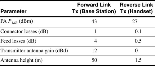
Table 3.3 repeats the receiver parameters from that same example. Antenna heights for the base station and mobile unit have been added to the tables. As in the Chapter 2 example, we will assume an operating frequency of 1900 MHz. (Technically this is just outside the range of validity of the Hata model.) We will also assume that the log-normal fading has a standard deviation of σpath = 8 dB. We will assume a large city environment, and our design will be expected to produce coverage of 90% of the cell area with 90% probability.
Table 3.3. Receiver Parameters for Example Link Budget
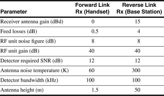
Solution
The Hata model for a large city is given by Equations (3.33) and (3.34). Substituting the frequency and the antenna heights gives median path loss as a function of distance from the transmitter:
Comparing Equation (3.163) with Equation (3.48) or Equation (3.154) shows that the path-loss exponent is v = 3.38.
Next we use the Reudink curves of Figure 3.21 to determine the required boundary coverage for an area coverage of 90%. Dividing the log-normal standard deviation by the path-loss exponent gives  . Entering Figure 3.21 with
  and Fu = 0.9 gives PPsens(R)0.75. Thus we need a 75% probability that the received signal power will exceed the receiver sensitivity at the cell boundary. Using this result in Equation (3.64) gives
where  is the receiver sensitivity and
  is the average received signal power at the cell boundary.
The receiver sensitivity was shown in Chapter 2 to depend primarily on the required signal-to-noise ratio at the detector, the receiver noise figure, the signal bandwidth, and the antenna noise temperature. In the Chapter 2 example the values given in Table 3.3 led to  for the forward link and
  for the reverse link. Equation (3.164) then gives
  for the forward link and
  for the reverse link.
Now we can put the pieces together by adding up the gains and losses, specifically,
where the antenna gains must be increased by 2.15 dB over the values given in Tables 3.2 and 3.3 to convert from dBd to dBi. As in the Chapter 2 example, we include a design margin of 3 dB. Substituting in Equation (3.165),
which gives  for the forward link. Similarly,
  for the reverse link.
Since the reverse link has the lower maximum path loss, the reverse link will determine the cell radius. Returning to the Hata model in Equation (3.163), we calculate the maximum cell size as 1.35 km. In Chapter 2 the maximum transmitter-receiver separation was calculated as 671 km. Including a real-world path-loss model and a fading margin has a significant effect on the predicted cell radius!
This chapter focused on propagation in the real world, and in particular on how this propagation can be modeled. Effective propagation models are necessary to provide system designers with the means to design reliable communication systems with a marketable quality of service at an affordable cost. In this section we present a brief review of the principal concepts introduced in this chapter.
In Chapters 2 and 3 we concentrated on the models a system designer uses to ensure an adequate received signal power for a single receiver located somewhere within, or moving through, a coverage area. In Chapter 4 we begin to consider the design of systems intended to provide service to many users. In particular, we introduce the cellular concept, which is intended to allow a virtually unlimited number of users to access a communication system that is limited in transmitted power and total available bandwidth.
A wireless system base station transmits a 20 W signal from an antenna located 20 m above a flat Earth. The base station antenna has a gain of 6 dBi and the system losses are 2 dB. A receiver is located in a delivery truck with an antenna atop the truck at 3 m above the ground. The receiving antenna gain is 2 dBi and the system operates at 1.2 GHz.
A. Find the received signal power when the truck is 20 km from the base station. Express your answer in decibels above a milliwatt. (Hint: Use Equation (3.25).)
B. What would the received signal power be in the absence of ground reflections?
C. Calculate the accuracy of the approximation of Equation (3.17) in reference to Equation (3.16).
Assume that the approximations made in Equations (3.9) and (3.10) are valid only for grazing angles of 1° or less. Using the ground reflections diagram illustrated in Figure 3.2 and the base station and receiving antenna heights of Problem 3.1, determine the minimum distance d between the base station and receiver for which Equations (3.9) and (3.10) (and subsequently Equation (3.24)) are valid. Using this distance, find the error resulting from using the approximation of Equation (3.17) for Equation (3.16). Express your answer in decibels relative to the value obtained from Equation (3.16).
A wireless system base station operating at 850 MHz transmits a 30 W signal from an antenna located atop a 30 m tower. The base station antenna gain is 6 dBi and the system losses, including cable and connector losses between the transmitter and the antenna terminals, are 3 dB. A handheld receiver has an antenna gain of 3 dBi and is carried at an average height of 1.6 m. The receiver has a bandwidth of 30 kHz and a noise figure of 9 dB.
A. In order to provide an adequate quality of service (QoS) the signal level at the input terminals of the receiver must be no less than 17 dB above thermal noise. Assuming an antenna temperature of 300 K and a flat Earth, calculate the maximum operating range.
B. What would be the maximum operating range if the base station and handheld receiver were located in free space?
Assume that the base station of Problem 3.3 is deployed at position A. Suppose that an identical base station is to be deployed at position B, as close as possible to position A without causing undue cochannel (same-frequency) interference. Specifically, assume that a handheld receiver as described in Problem 3.3 is operating along the line joining A and B, and that at the maximum distance from A as determined in Problem 3.3, the signal-to-noise-and-interference ratio must be at least 16 dB (that is, 1 dB of interference is allowed). Assuming a flat Earth, find the minimum distance between A and B.
A wireless system base station operating at 1.2 GHz in an urban environment transmits 15 W from the top of a 30 m tower. The base station antenna's gain is 7 dBi and the system losses are 4 dB. A receiver operating in the vicinity of the base station is located at an average height of 1.6 m above a flat Earth and has an antenna gain of 2 dBi.
A. Calculate the median path loss when the receiver is 12 km from the base station using the Hata model.
B. Calculate the received signal power.
C. Calculate the received signal power using Equation (3.25) for the same range. Compare with your answer to part B and discuss the difference.
Assume that for the system of Problem 3.5 the receiver has a 30 kHz bandwidth and a 6 dB noise figure and operates in an environment that produces an antenna noise temperature of 290 K. The QoS objectives require at least 18 dB SNR.
A. Find the maximum operating range using the Hata model.
B. Find the maximum operating range using Equation (3.25) and discuss the difference.
Find the maximum operating range of the system described in Problem 3.5 and Problem 3.6 for suburban and rural environments.
Calculate the median path loss for the system of Problem 3.5 using the Lee model and the parameters describing New York City.
Find the maximum operating range for the system described in Problem 3.5 and Problem 3.6 using the Lee model for New York City. Compare the result with that of the Hata model and discuss the reasons for the difference.
The QoS for a certain system requires that the received signal power be greater than the receiver sensitivity level with probability PQ. Express PQ in terms of the fade margin  and standard deviation of the path loss, σpath.
A certain receiver has a thermal noise floor of -110 dBm. Suppose that the receiver requires a 15 dB SNR in order to adequately replicate the transmitted signal. The QoS objective requires that the received signal be above the receiver sensitivity level 85% of the time. Assuming σpath = 7 dB, find the required fade margin in decibels. What is the minimum median signal level required at the receiver input to meet the QoS objective?
A base station operating at 1.8 GHz transmits a 44 dBm signal from an antenna located at 100 ft (effective height) above the pavement in urban Philadelphia. The transmitting antenna has a gain of 4 dBi and there are 2 dB of system losses between the transmitter and its antenna. The receiving antenna has a gain of 2 dBi and is located on the roof of a car 5 ft above the pavement.
A. Assuming that σpath = 8 dB, calculate the probability that the received signal power is 10 dB above the median value at 10 mi. Use the Lee model.
B. Find the probability that the received signal power at 5 mi is greater than 10 dB above the median value at 10 mi.
Assume that the receiver of Problem 3.12 has a bandwidth of 200 kHz and a noise figure of 6 dB operating with an antenna noise temperature of 290 K. What is the maximum operating range for which there is a 90% probability that the received signal level is 15 dB above the receiver's thermal noise floor?
A public safety system has the following parameters:
Base station transmitter power = 35 W
Base station transmitting antenna gain = 6 dBi
Operating frequency = 1.2 GHz
System losses = 3 dB
Receiving antenna gain = 3 dBi
Receiving antenna height = 1.6 m
Receiver bandwidth = 30 kHz
Receiver noise figure = 4 dB
Antenna noise temperature = 290 K
The system is to be used in medium-sized city environments with σpath = 6 dB. Adequate intelligibility of emergency communications requires that the received signal power be 12 dB above the receiver's noise floor (i.e., SNR = 12 dB).
A. Find the fade margin required to ensure that the received signal power is above the receiver sensitivity level with 95% probability.
B. Find the median signal level required to meet the 95% QoS objective.
C. What is the minimum effective height of the transmitting antenna required to achieve the QoS objective at 8 km? Use the Hata model.
Using Equation (3.80), show that the peaks of a two-ray model occur at
and the nulls occur at
where f0 is the frequency for which λ0 = d2 - d1, the path difference, and Δ Φ = Φ2 - Φ1.
A. What is the peak-to-peak (or null-to-null) frequency difference?
B. Verify that the expression for the peaks predicts the values observable in Figure 3.6.
What is the probability that a signal in a multipath environment exceeds its average power level?
By how many decibels must the average SNR exceed the minimum SNR to achieve a 95% probability that the received SNR will be above the minimum in a multipath environment?
A certain multipath channel has the power delay spread shown in Figure P 3.1, where  ,
,  ,
,  , and the corresponding times are t1 = 3 μs, t2 = 4 μs, and t3 = 6 μs. Approximate the maximum system data rate that can be supported without the need for equalization.
Figure P 3.1. A Power Delay Spread Function
A modern digital wireless communication system transmits at a center frequency of 1.9 GHz and has a bandwidth of 1.25 MHz and a data rate of 1.2288 Mbits/s. Assume that there are two signal paths that differ in amplitude by 1 dB and in phase by  . The receiver is moving at 60 mph and the signals arrive at -5° and 85° with respect to the direction of travel.
A. What is the Doppler spread?
B. What is the period of a fading cycle?
C. Is the fading fast or slow with respect to the signal? How fast would the receiver have to be moving to experience fast fading?
The sensitivity of a certain receiver is –104 dBm. The receiver is to be used in an urban environment where the path-loss exponent is 4.2 and σpath = 9 dB. The system deployment criteria require that the received signal be above the receiver sensitivity over at least 90% of the coverage area. What is the required fade margin?