The previous two chapters presented the fundamental concepts underlying the behavior of radio frequency propagation in a real-world environment. With these principles as a foundation, we return to the development of a solution to the general systems-engineering challenge posed in Chapter 1, that is, to design a wireless telecommunication system that will
The challenge as we have stated it is broad and devoid of any quantitative specification of the system's attributes. Nevertheless, the problem statement is not unlike one that a company might pose in the initial stages of developing a product or service.
Product or service development requires the investment of money, physical resources, and people. Sound business practice requires a clear assessment of the benefits to be gained by making the investment. The financial "return on investment" is often used to determine the viability of an investment in a new product or service. Based on an assessment of the return on investment, an enterprise (or, more accurately, the investors in the enterprise) can make informed decisions about the efficacy of proceeding with a new venture. This assessment may include quantifying the market opportunity in terms of the likely number of subscribers and the projected rate of growth in that number, the subscribers' willingness to pay for the service, the time to market (how long it will take to develop the service or product), the estimated cost of development, the projected profit margin, the product life cycle, and the competitive ability of companies offering similar products or services.
As discussed in Chapter 1, systems engineers play an important role, especially in the early process stages. As members of the product definition team, they represent the technical community, providing the insights necessary to ensure that the product concept is realistic and well defined. Systems engineers work with the business team to provide a complete, detailed, and quantitative definition of the product or service to be developed. This usually requires a strong interaction among the members of the technical community to ensure that the required technical competencies are available, the budget and schedule are realistic, and the technical risks are noted and realistically appraised.
Once a product or service has been defined in sufficient detail, key product requirements are assessed and analyzed to determine the high-level design or "system architecture" that best supports the project goals, within the constraints of resources, budget, and schedule. Simulations may be performed to estimate performance and the trade-off of performance against cost for various architectural alternatives under project constraints.
A system architecture may include a high-level technical description of the system and major subsystems along with their key functions and parameters. Development of a system architecture is often led by systems engineers working in collaboration with appropriate members of the technical team and the business team. In the next section we consider the overall system approach, or architecture, that might be used to implement the key characteristics of the system identified in our problem statement.
As we proceed to investigate solutions to our stated problem, we will introduce some of the specific parameters and characteristics encountered in modern systems. We will also introduce realistic constraints as they are needed and when sufficient background has been presented to make them meaningful.
As a first consideration, we note that the allowable frequency range over which a proposed system may operate is usually fixed by government regulation and, in some cases, by international treaties. This implies that the operating frequency bands are finite and predetermined. In the United States, civilian communications policy is administered by the FCC, an agency created by Congress in 1934. Communications regulations are published in Volume 47 of the Code of Federal Regulations (CFR). The regulations pertaining to unlicensed radio services appear in Part 15 (designated 47CFR15). Each licensed radio service has its own part. Wireless services are assigned specific frequency bands to limit interference and ensure the reliability of communication services. Emission of radio frequency energy outside of the assigned frequency band must be limited in accordance with the rules governing the license. Licenses may also impose restrictions that vary by geographic area.
In most cases a wireless service is assigned a continuous range of frequencies. Let us designate this range as fsl to fsu, where fsl and fsu are the lower and upper limits, respectively, of the operating frequency range. Let the system bandwidth be denoted Bsys, where Bsys = fsu - fsl. The fraction of this bandwidth to be used by an individual subscriber depends on the information source (speech, music, data, video, etc.) and on the quality of service to be supported. We suppose that the band fsl to fsu is divided into Nchan subbands or "channels," each of bandwidth Bchan. We understand Bchan to be the minimum bandwidth required to convey the required information in both directions at the required quality of service (QoS) between two endpoints. Let the center frequency of each channel be given by
To simplify our discussions we also assume that each channel can support only one two-way radio link between a pair of endpoints at any instant of time. Therefore only Nchan simultaneous radio connections can be supported in the given spectrum Bsys. For systems of interest to us Bchan is much smaller than Bsys, so there are many available channels.
Example
Radio spectrum is a limited resource. Like land, "they aren't making any more of it." Although new technology allows the use of ever higher frequencies, the general pattern is that spectrum can be assigned to a new radio service only if it is taken away from an existing radio service. In 1983 the FCC allocated 40 MHz of spectrum for a new cellular telephone system. Six years later an additional 10 MHz was added. The allocated spectrum is in the bands 824–849 MHz and 869–894 MHz. This spectrum had previously been allocated to UHF television but became available when the spread of cable television reduced some of the demand for large numbers of broadcasting channels.
Each channel in the Advanced Mobile Phone Service (AMPS) consists of a 30 kHz "forward" link from the base station to the mobile unit and a 30 kHz "reverse" link from the mobile unit to the base station. All of the reverse links are contained in the band 824–849 MHz, and all of the forward links are in the band 869–894 MHz. In each two-way channel, the forward and reverse subchannels are separated by 45 MHz.
Systems that divide an allocated spectrum into channels that are to be shared among many users (as described previously) are classified as frequency-division multiple access (FDMA) or frequency-division multiplexing (FDM) systems. There are other ways to allocate channels among many users. For example, the entire spectrum allocation may be dedicated to a single user for a short period of time, with multiple users taking turns on a round-robin basis. In a later chapter we will discuss this approach and other alternatives for implementing multiple access. Our intention in this chapter is to focus on the cellular concept, a concept that is perhaps most easily understood in the context of an FDMA system.
Given a system bandwidth Bsys and a channel bandwidth Bchan, the number of distinct channels available is
It should be self-evident that the number of subscribers that a system can support is related to the number of available channels. The actual relationship between number of users and Nchan, however, is not so obvious. In a telephone system no user occupies a channel continuously, so a channel can support more than one user. In general, the number of users that can be supported is much greater than the number of channels. We will find that user behavior plays an important role in determining the ultimate capacity of an Nchan-channel system. In the early stages of development of the public telephone system, it was recognized that a direct connection between every pair of subscribers was impractical and unnecessary. The concept of "traffic engineering"—that is, planning the allocation of resources to allow these resources to be effectively shared—is central to the design of multiple-user systems. We will discuss the basics of traffic engineering later in this chapter, at which time we will answer the question of how many subscribers Nchan channels can support.
The simplest architecture for a wireless system might be to locate a single base station near the center of a coverage area and to adjust the transmitted power level and antenna height so that signal levels are sufficient to ensure the required quality of service within the coverage area. This is the common configuration for radio systems serving police and fire departments and for tow-truck and taxicab companies. Early mobile telephone systems were also designed along these lines. The Improved Mobile Telephone Service (IMTS), introduced in the 1950s and 1960s, is an example. Unfortunately by 1976 the IMTS system in New York City, operating with 12 channels, was able to serve only about 500 paying customers. There was a waiting list of over 3700 people, and service was poor owing to the high blocking (system busy) rate.
Although the number of subscribers (and the quality of service) could be increased by adding channels, systems of this design are limited in coverage area by the maximum practical transmitter power and the sensitivity of the receiver. This kind of system is referred to as being "noise limited." The performance within a given coverage area can be increased by adding repeater base stations, but doing so increases the cost of the service without increasing the number of customers who will share that cost. Increasing the coverage area may increase the number of potential customers, but without increasing the system's ability to provide them service. Without additional spectrum, adding more customers will degrade the system blocking rate. Clearly, neither of the goals of being capable of expanding in geographic coverage or allowing for virtually limitless growth in the number of users can be met with this approach.
Since spectrum is limited, the most promising avenue for increasing the number of users is to utilize the available spectrum more efficiently. Specifically, we wish to increase the number of subscribers who can simultaneously use a given channel within the specified coverage area. Normally, allowing multiple users to transmit on the same channel at the same time increases interference. The key, then, is to find ways to reduce, or eliminate, this so-called cochannel interference. One approach might be to geographically isolate the users of a given channel by physically separating them. This is the basic concept underlying development of the first cellular systems.
Suppose instead of a single high-powered, centrally located base station we envision many low-powered base stations, each serving only a portion of the desired coverage area. The smaller coverage area served by a single base station is called a cell. Since the area of a cell is small, each cell will contain only a limited number of subscribers. We can therefore distribute the available channels among the cells so that each cell has only a subset of the complete set of channels. Now if two cells are far enough apart, they can be assigned the same group of channels. This allows every channel to be reused, possibly many times, throughout the system's coverage area. If the same channel supports two different customers at the same time in different parts of the system, however, there is a potential for cochannel interference. We shall see that the system's ability to withstand cochannel interference and the size of the cells are the limiting factors in determining the number of subscribers that can be supported. A system with this configuration is said to be "interference limited." An important consequence of dividing the service area into cells is the need to transfer a call from one base station to another as a mobile unit moves through the service area. This transfer is called a "handoff" or "handover" and will be discussed in a subsequent section of this chapter. In the next section we will describe the cellular concept in some detail and demonstrate its ability to provide substantial, if not limitless, growth in both coverage and user capacity.
Interference control is the key to allowing reuse of channels within a given geographic area. We therefore begin our discussion of cellular concepts by developing a simple model to predict the interference levels caused by geographically separated transmitters operating on a common channel.
Consider two cells whose base stations (BS1 and BS2 respectively) are separated by a distance D. Each base station has a circular coverage area of radius R as shown in Figure 4.1. Assume that the propagation environment is uniform within and completely surrounding the two cells and that the path-loss exponent is v. Let the two base stations receive on the same channel, with center frequency f1. Also shown in Figure 4.1 are two mobile units, MU1 and MU2, served by base stations BS1 and BS2 respectively. The mobile units are located at the boundaries of their respective cells, each at distance R from its base station. To keep the discussion simple, we consider transmission on the reverse channel, from mobile unit to base station, only.
Figure 4.1. Cochannel Interference from a Single Source
From our work in Chapter 3, the level of the signal received at base station BS1 from mobile unit MU1 can be expressed as

where K1 is a constant that incorporates the transmitter power, the antenna gains, the antenna heights, and so on. The received signal level at base station BS1 from mobile unit MU2 can be written
Now from the perspective of base station BS1, P1 represents "signal" and P2 is cochannel interference. The signal-to-noise-and-interference ratio at base station BS1 is
where Pn is thermal noise referred to the base station input. When the receiver noise is significantly greater than the interference—that is, when Pn  P2—we describe the system as "noise limited," as explained earlier. For this case,
When the received noise is significantly less than the interference—that is, when Pn  P2—the system is "interference limited." Then we can write
For identical mobile units transmitting at the same power level, Equation (4.7) becomes

The locations of the mobile units in Figure 4.1 have been chosen to illustrate the worst case of signal-to-interference ratio (SIR). Mobile unit MU1 is at the perimeter of its cell, as far as possible from the base station serving it. Mobile unit MU2 is also at the perimeter of its cell, as close to base station BS1 as it can get while remaining in the cell served by BS2. It should be evident that for this geometry the signal-to-interference ratio would be the same if we calculated it at base station BS2 or at either mobile unit.
In a realistic cellular system there are likely to be more than two cells, and cochannel interference may come from more than one source. If there are J cells surrounding base station BS1, each containing a mobile unit, and all of these mobile units are transmitting on the same channel, then the signal-to-interference ratio at BS1 can be written
where Pj, j = 2,...,J + 1 represent cochannel interference from mobile units in the surrounding cells. In the discussion that follows, we will see that in the most important case all of the interference sources are identical, and all are located at distances approximately D from the base station BS1 receiver. In this case Equation (4.9) becomes
Equation (4.10) suggests that the ratio of separation distance D to cell radius R is the predominant factor in determining the signal-to-interference ratio  . The ratio
  is usually termed the "frequency reuse ratio" or the "interference reduction factor." Quality of service objectives for the cellular system will usually dictate that some minimum signal-to-interference ratio, say, S/I = γmin, be met throughout the area. This normally implies that D must exceed R by some factor greater than 1. Base stations BS1 and BS2 are then separated by enough distance that additional cells can be deployed between them. To avoid increasing the cochannel interference, these additional cells must operate on channel frequencies other than f1. In this way an entire geographic area can receive contiguous coverage, while allowing frequency reuse at an acceptable level of cochannel interference.
When the number of available channels Nchan is sufficiently large, the channels may be organized into groups called "channel sets," Fi, i = 1,..., N, and deployed among the cells as suggested by Figure 4.2. The assignment of sets of frequencies to each cell allows more than one subscriber to be serviced at a time in any given cell. The appropriate size of a channel set and the number of distinct channel sets then become design parameters.
Figure 4.2. Deployment of Channel Sets in Neighboring Cells
In the single-base-station approach, popular before the introduction of frequency reuse, the location of users within the coverage area was not a matter of concern. In a cellular system the geographical distribution of users may matter. Since the allocated group of channels is broken up into channel sets, each cell can service only a limited number of customers. If all of the customers happen to congregate in a single cell, it is likely that there will not be enough channels available in that cell to provide adequate service. In real-world cellular systems the downtown areas of cities are more likely to experience a higher density of customers, at least during the working day, than are the peripheral areas. The higher customer density in some cells can be managed either by assigning more channels to these cells or by making these cells smaller so that they include fewer customers. Increasing the number of channels in a channel set causes a decrease in the number of channel sets that are available. The geometry of Figure 4.2 suggests that as the number of channel sets decreases, so does the separation distance D, leading to an increase in cochannel interference. On the other hand, decreasing the cell radius R requires more cells to cover the market area, leading to an increased investment in base station towers and transmitters. These considerations will be examined in detail later. For the present we will accept the simplest case and assume that subscribers are uniformly distributed throughout the market area.
Our design objectives require that the cellular system be capable of growth in both coverage area and user capacity. This implies that our system must have an ability to add cells to the periphery to expand the service area, and also an ability to add cells within the coverage area to increase the user capacity. It is certainly possible to lay out cells and assign channels in a way that is individually crafted for a given geographic area and customer distribution, but adding new cells for growth would then require custom reengineering. Such ad-hoc design could easily result in a need to redistribute cells and relocate base stations. Construction of a base station is costly and, in addition to the cost of erecting a tower, may involve the purchase of real estate and the approval of zoning boards. Consequently the capability to expand must be designed into the cellular system from the beginning. To facilitate expansion it is convenient to deploy cells that are uniform in shape and are located on a symmetric grid. We will now investigate the extent to which such a regular layout is possible and the principles on which the cell layout is based.
Given a specified service area, placing cells to cover that area requires that some assumption be made about the shape of the coverage regions of the individual base stations. The simplest assumption is that coverage regions will be circular, based on the principle that equal-level signal contours surrounding a transmitting antenna are circles with the base station at the origin. Given what we know about propagation, however, it is unlikely that real-world coverage areas will be circular in any but a statistical sense. In any specific instance, the shape of a coverage region is not circular but is rather somewhat amorphous and highly dependent on terrain and the location of surrounding obstacles. Keep in mind, however, that our objective in configuring cells is to provide a high likelihood that a mobile unit will be adequately served by its nearest base station. To accomplish this purpose, determining the shape of the actual coverage area is not as important as defining the boundaries over which the mobile unit will operate while communicating with the specific base station. Our approach, then, is to initially assume that the base station coverage areas are circular and to focus on developing an efficient method for locating and growing the cells. Historical experience has shown that once the cells are deployed, system parameters may be adjusted to provide adequate performance in the vast majority of circumstances without the need for extraordinary engineering efforts.
Although we will assume that the coverage regions are circular, a little reflection will show that it is not possible to uniformly cover a geographic area with circles without having gaps or overlaps in coverage. We naturally seek to determine a layout pattern that has no gaps. Also, to ensure that the number of cells deployed is minimal, we wish to minimize the overlaps. Figure 4.3 shows two overlapping circular coverage regions. In the region of overlap there is a straight-line boundary that divides the locations for which the signal from base station BS1 is stronger than the signal from base station BS2 and vice versa. Consequently, if we cover our market area with overlapping circular coverage regions arranged on some kind of a regular grid, the actual cells will be polygons. Now it turns out that there are only three regular polygonal shapes for which it is possible to completely "tile" an area without overlaps or gaps. These shapes are the equilateral triangle, the square, and the hexagon: regular polygons of three, four, or six sides, respectively. Figure 4.4 shows the tile pattern for each of these polygons and also shows how a single polygon can be inscribed in a circle of radius R, the cell (or coverage) radius. Observe that within the circle of radius R the area covered by the hexagonal pattern is greatest.
Figure 4.3. The Boundary between Two Circular Cells
Figure 4.4. Covering a Plane Area with Regular Polygons: (a) Equilateral Triangles; (b) Squares; (c) Hexagons
Also observe that overlap is minimized when circular cells are deployed along a hexagonal grid as is shown in Figure 4.5. The hexagonal layout is evidently the most economically efficient one, as it requires the fewest cells to cover a given area. For these reasons, a hexagonal cell layout is chosen as the basis for designing cellular systems. In the discussion that follows, we will treat cells as having hexagonal shapes. Although this is never precisely true in fact, the assumption provides a means for developing concepts about frequency reuse and cell size that may be applied in practice. Further, the hexagonal layout does provide a starting point for real-world design. We therefore proceed to discuss the geometrical properties of a hexagonal grid as they relate to cell layout and frequency reuse.
Figure 4.5. Overlap in Circular Cells Using a (a) Triangular Grid; (b) Rectangular Grid; (c) Hexagonal Grid

Figure 4.6 shows a hexagonal cell and some of its neighbors. We assume that all of the cells have radius R and that the base stations are located in the centers of the cells. The hexagonal geometry dictates that adjacent cells are located at multiples of 60° surrounding any given cell, and the separation between adjacent cell centers is  . Following V. H. MacDonald[1], we locate position in the array of cells by choosing a coordinate system (u, v) such that the positive coordinate axes intersect at a 60° angle and the unit distance along either axis is equal to , which is the separation between adjacent cells. Figure 4.7 shows these coordinate axes. The normalized distance
  between any two arbitrary cells whose centers are located at the coordinates (u1, v1) and (u2, v2) can be found using the law of cosines as illustrated in Figure 4.8. We obtain
Figure 4.6. Adjacent Cell Geometry
Figure 4.7. Coordinate System for Hexagonal Layout
Figure 4.8. Computation of Separation Distance
The actual distance D between the cell centers is given by

since actual and normalized distance are related by the scale factor  . In terms of normalized distance, the lengths along the axes between u1 and u2 and between v1 and v2 are integers. We can let u2 - u1 = i and v2 - v1 = j. In terms of i and J, Equation (4.11) becomes

If we choose the center of any cell as a reference location, then the distance to the center of any other cell can be expressed as a function (i, j) of the integers i and j. The orientation of the coordinate system is arbitrary, so that for any i and j there will be six cells whose centers lie at distance (i, j) from the reference. These cells will surround the reference at multiples of 60°.
Figure 4.9 illustrates this geometry for the case i = 2, j = 2,  . Note that the centers of the six cells at distance D(i, j) from the reference form the corners of a large hexagon whose radius and sides have lengths equal to the separation distance (i, j). The location of any one of the six corners of the large hexagon can be found by starting at the reference point, moving i cells in a direction perpendicular to any side of the reference cell, turning counterclockwise 60°, and moving j cells in the new direction. (Similar results are obtained by turning clockwise instead of counterclockwise, or by moving j cells before moving i cells; however, the first method is usually adopted by convention.)
Figure 4.9. Cells at Distance  from a Reference Cell
Recall from our discussion following Equation (4.10) that the signal-to-interference ratio S/I is determined by the frequency reuse ratio Q = D/R, where D is the distance between a pair of cells that use the same set of channels. In the hexagonal geometry, Equation (4.12) shows that the frequency reuse ratio (and therefore the signal-to-interference ratio) is actually determined by the normalized distance between the cells, that is,

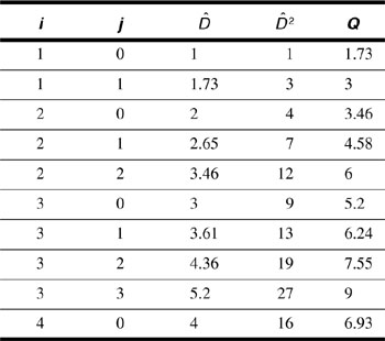
If we choose a particular cell as our reference, we can use the required signal-to-interference ratio to determine a minimum separation distance between cells that use the same channel set. Once is established, we can use Equation (4.13) to find corresponding integers i and j and then use these integers to locate all of the neighboring cells that reuse the same set of channels. Table 4.1 lists some representative values of the location integers i and j, the corresponding values of given by Equation (4.13), the values of  (we will need this later), and the frequency reuse ratios given by Equation (4.14). Notice that because i and j are integers, only certain distances are physically possible. This means that only certain values of frequency reuse ratio Q are possible as well. If the signal-to-interference ratio requirement leads to a required value of Q that is not achievable, then the next higher value that is achievable must be used.
Table 4.1. Tabulation of Values of Normalized Distance and Frequency Reuse Ratio
We observed earlier that the required distance between cells that share the same channel set is usually large enough that there are cells in between that can use other channel sets. This suggests the following procedure for assigning channels to cells. Choose any cell and assign to it channel set F1. Call this cell A. Using the procedure described previously, use the location integers i and j to identify all the cells that can use channel set F1. Label all of these cell A. Now choose any unlabeled cell and assign to it channel set F2. Label this cell B. Using the same i and j, locate all cells that can be assigned channel set F2 and label them B. Continue this procedure until all cells have been assigned a channel set and labeled. A collection of contiguous cells, A, B, C, ..., that between them account for all of the channel sets is called a cluster. We will use the symbol Kcluster to designate the number of cells in a cluster. This procedure is illustrated in Figure 4.10 for a reuse distance = 2, which corresponds to i = 2, j = 0. For the layout of the figure, we find that Kcluster = 4.
Figure 4.10. Cell Layout Process for Reuse Distance (2,0) = 2, Producing a Four-Cell Cluster
Since each cell in a cluster is assigned a unique channel set, and all of the channels sets are accounted for, there must be Kcluster distinct channel sets. If the system has an allocation of Nchan channels, then the number of channels in a channel set—that is, the number of channels in a cell—is Ncell given by
It is important to realize that each cluster has all Nchan channels available, and that these channels are reused in every cluster. If the entire market area is covered by M clusters of cells, then the total number Nmarket of channels available to subscribers is given by
Two things should now be apparent: First, the number of subscribers that the entire system can accommodate can be vastly larger than the number Nchan of channels, since the same channel can be used simultaneously by different subscribers in different locations in the system. Second, to increase the geographic area covered by the cellular system, it is necessary only to add clusters of cells around the periphery. Since adding new clusters of cells increases M, the number Nmarket of available channels is also increased. Thus the added geographic area can bring in additional customers without increasing the usage burden on the channels.
Intuitively one might expect that the number Kcluster of cells in a cluster is related to the reuse distance . A large distance implies that many cells lie between "cochannel" cells that use the same channel set. This suggests that the cluster size should also be large. To make this intuitive picture more precise, we determine the relationship between Kcluster and . First note that a hexagon of radius R has an area Acell given by
Next, choose an arbitrary reference cell, call it cell A, and identify the six surrounding cells (also A) that share the same channel set. Recall that the centers of the six cochannel cells form a large hexagon, with normalized radius or actual radius D. The geometry is shown in Figure 4.9 and also in Figure 4.10(c). The large hexagon has an area Ahex given by
Now we need to determine how many clusters are contained inside the large hexagon. We can associate a cluster with each cell A, but some of these clusters are only partially contained in the large hexagon. Figure 4.10(c) shows a typical situation. There will always be one complete cluster associated with the reference cell inside the large hexagon. The sides of the large hexagon meet at each vertex at an angle of 120°. Three of these vertices include an additional complete cluster. The remaining three vertices include a third complete cluster. Thus the large hexagon always includes three complete clusters regardless of the particular value of . Figure 4.11 shows the three clusters for the case = 2. The last step is to put the pieces together. The area of the large hexagon is given by Equation (4.18). Dividing by three gives the area of one cluster:
Figure 4.11. Every Large Hexagon Contains Three Clusters
Dividing the area of a cluster by the area of a cell gives the number of cells per cluster:
This result can also be written
Finally, substituting Equation (4.12) into Equation (4.20) gives
Equation (4.22) explains the importance of the column in Table 4.1.
Example
Suppose signal-to-interference considerations require a frequency reuse ratio of at least Q = 4.0. Find the minimum cluster size and draw the pattern of cells, showing at least one cluster.
Solution
Equation (4.14) and Equation (4.13) give  with
with  . No combination of integer values for i and j will give a value for Q of 4.0. Rounding up to the nearest acceptable value gives
  and
and  , with i = 2 and j = 1. (See Table 4.1.) Then Equation (4.22) gives Kcluster = = 7. Figure 4.12 shows a seven-cell cluster and some cochannel cells of channel set A.
Figure 4.12. A Seven-Cell Cluster
Example
A market area for a cellular system is covered by 63 cells organized into 9-cell clusters. The system is allocated enough radio spectrum to support Nchan = 800 channels. Determine the percentage increase in the number of channels available to subscribers Nmarket if the cluster size is reduced to Kcluster = 7. What might limit reducing the cluster size still further?
Solution
Using Equation (4.16) with  gives Nmarket = 7 x 800 = 5600 channels. If the cluster size is reduced to 7, then
  , and Nmarket = 9 x 800 = 7200 channels. The percentage increase is
  .
.
Reducing the cluster size reduces the distance between cochannel cells, raising the level of cochannel interference. Cochannel interference provides the limit on how small the cluster size can be. Equation (4.21) shows how the cluster size is related to the frequency reuse ratio. In the next section we will establish the quantitative relationship between frequency reuse ratio and signal-to-interference ratio.
The final example of the previous section showed that for a given cell size, the number of customers that a cellular system can support is maximized if the cluster size is minimum. Cochannel interference was seen to be the factor that limits the extent to which cluster size can be reduced, since reducing the cluster size has the effect of reducing the frequency reuse ratio Q = D/R. In this section we will explore the relation between the frequency reuse ratio and the signal-to-interference ratio. We will then introduce the concept of adjacent-channel interference, which also has an effect on efficient frequency reuse.
The first U.S. cellular system, AMPS, was designed with the goal of approximating "toll quality" speech communications using analog modulation. Toll quality refers to a subjective evaluation of the quality of long-distance wired communications in the public switched telephone network. The speech quality is measured by tests in which a number of people assess specific speech samples to develop a "mean opinion score" for each sample. To determine AMPS system parameters, systems engineers developed simulators that mimicked a typical signal as corrupted by fading, noise, and interference. These simulators were used to conduct tests to determine minimum signal-to-noise and signal-to-interference ratios that would allow the quality of service objectives to be met. The results of these early studies determined that quality objectives could be met under these conditions.
Modern systems are predominantly digital and are capable of communicating many types of information in addition to speech. QoS metrics can be defined for each information type and used to determine the required signal-to-noise and signal-to-interference ratios.
We begin our analysis by considering the interference from the nearest cochannel base stations as shown in Figure 4.13. Although the diagram depicts a seven-cell cluster, the results apply to clusters of any size. We assume that the receiver noise is negligible compared to the interference. The reference base station is in the center of the diagram.
Figure 4.13. First-Tier Cochannel Interference Sources
As a first approximation, consider that a mobile unit is located on the cell boundary at a distance equal to the cell radius R from the reference base station. This is the farthest that a mobile unit should be from its serving base station. The nearest cochannel sources are mobile units in the cochannel cells and are all approximately at the reuse distance D from the reference base station. The signal-to-interference ratio S/I is given by Equation (4.9) with J = 6 interference sources:

Now if all of the mobile units have the same parameters and the environment is uniform in all directions, then
If we further assume that the path-loss exponent is v, then
where Q is the frequency reuse factor. Using Equation (4.21),
Example
Suppose, as in the AMPS system, that a signal-to-interference ratio of 18 dB is required. The path-loss exponent is v = 4.0. Considering only the nearest cochannel interference sources, find the minimum cluster size.
Solution
 means
means  . Using Equation (4.26),
  , so Kcluster = 6.49. A check of Table 4.1 shows that the nearest admissible cluster size larger than 6.49 is Kcluster = 7, achieved with i = 2, j = 1.
Table 4.2 repeats the information shown in Table 4.1 but includes a column of values of signal-to-interference ratio assuming that the path-loss exponent v = 4. Only first-tier interference is taken into account, but the first-tier interference predominates. In the presence of a deep fade, or when no first-tier sources are present, interference from second or further tiers may be noticeable.
Table 4.2. Approximate Signal-to-Interference Ratio for Several Reuse Ratios with v = 4
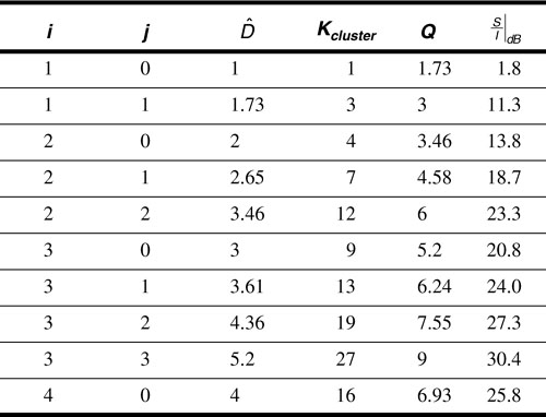
Figure 4.14 shows the geometry of the second and third cochannel interference tiers. The second-tier radius is the center-to-center distance between large hexagons, that is,
Figure 4.14. First-, Second-, and Third-Tier Cochannel Interference

From the geometry, the third-tier radius is simply double the side of a large hexagon, or

For a path-loss exponent of v = 4, interference from the second tier is
indicating that the interference from the second tier is 9.54 dB below the level of interference from the first tier. Similarly, the interference from the third tier is 12 dB below the first-tier level. It is rarely necessary to consider interference from tiers farther out, but it may be necessary to do so in situations where the fading is exceptionally severe, or where the propagation environment has a small or widely varying path-loss exponent. Should the need to consider additional tiers of interference arise, the method presented is directly applicable.
Adjacent-channel interference is interference to a receiver listening on a given channel from a transmission occurring on an adjacent channel. A cellular receiver must be designed to receive on all channels in the cellular system band, as a particular telephone connection may be assigned to any of the possible channels. The receiver separates one channel from another by using a highly selective filter. The passband bandwidth of the filter is equal to the channel bandwidth. The filter must cut off sharply at the passband edges, so that signals in the adjacent channels will not be passed to the demodulator. Now a "brick wall" filter, which cuts off abruptly and completely at the passband edges, is a physical impossibility. It turns out, moreover, that sharp cutoff filters may be far too expensive for mass consumer markets. Analog filters require a large number of components to achieve high selectivity (sharp cutoff). Also, for both analog and digital implementations, the performance of a sharp cutoff filter is very sensitive to small errors in the component or coefficient values.
Figure 4.15 shows the frequency response of a tenth-order Chebyshev filter with a 30 kHz passband. The center frequency has been arbitrarily selected as 870.03 MHz. This frequency response is not intended to represent any specific manufacturer's equipment but to suggest what a selective bandpass frequency response might look like. Notice from the figure that this filter produces an attenuation of about 50 dB at the center of the adjacent channels, 30 kHz above or below the filter's center frequency. One might imagine that 50 dB of attenuation in the adjacent channel might be enough to render interference from these channels negligible. The following example illustrates that the situation might be otherwise.
Figure 4.15. A Selective Bandpass Filter

Example
A base station receiver in an urban environment is receiving two signals from mobile units, one desired and one in an adjacent channel. The mobile units use identical equipment and are transmitting at equal power levels; the path-loss exponent is v = 4. The distance from the desired mobile unit to the base station is d1, and the distance from the interfering mobile unit to the base station is d1/20. (This would be the situation, for example, if the desired mobile unit were one mile from the base station and the interfering mobile unit were one city block from the base station.) If the base station uses a filter like the one shown in Figure 4.15 to separate signals, find the relative power levels of the two received signals after filtering.
Solution
As in Equation (4.3), we can write the received power from the desired mobile unit as

and the received power from the interfering mobile unit as

In decibels we have
Now the filter of Figure 4.15 passes the desired signal essentially without attenuation, but it attenuates the interfering signal. The amount of attenuation varies with frequency, but for a rough calculation we can take the attenuation at the center of the channel as typical. From Figure 4.15 we see that this attenuation is about 50 dB. Therefore at the filter output, the desired and interfering signals have about equal power.
We can see from the example that adjacent-channel interference can be a problem, even with highly selective channel filtering. Several strategies are available for dealing with this problem.
A common strategy in the broadcast services is to avoid using adjacent channels in the same market area. This strategy is used in both AM and FM broadcasting and in television. In cellular systems, however, the number of channels available translates directly into the number of customers who can be supported, which, in turn, translates directly into revenue. Channels are too valuable to be set aside for interference avoidance.
The power level of a mobile unit transmitter can be controlled dynamically, so that it transmits less power when it is nearer the base station than it does when it is at a cell edge. Power control has been in use in some form since the earliest cellular systems. In modern cellular systems a mobile unit's transmitted power is adjusted in 1 dB increments every few milliseconds, to keep the power level received at a base station constant as the mobile unit moves over the cell's coverage area.
Finally, channels can be partitioned so that adjacent channels are not assigned to the same cell or to cells that are immediate neighbors. This will guarantee that an interference source cannot get physically close to a base station receiver. When cluster sizes are small, however, the available channels will be divided up among a relatively small number of cells. In this case it may be difficult to avoid assigning adjacent channels to the same or nearby cells, and adjacent-channel interference may significantly limit how small the clusters can be made.
We have seen how the concept of frequency reuse leads to a cellular architecture that can allow for almost limitless expansion in the geographic area and the number of subscribers that the system can service. In configuring a cellular layout two parameters are of key importance; these are the cell radius R and the cluster size Kcluster. We begin this section by summarizing the design trade-offs in which these parameters are central. We will then focus on issues regarding system expansion. Although a cellular system can be expanded in geographic coverage simply by adding cells at the periphery, we have not addressed how a system can expand in user density. Since the history of cellular telephones has been characterized by rapid growth, the experience of all cellular start-ups has been a rapid expansion in subscribers. We will discuss two methods for dealing with an increasing subscriber density: sectoring and cell splitting.
The cell radius governs both the geographic area covered by a cell and also, for a given subscriber density, the number of subscribers that the cell must service. Simple economic considerations suggest that the cell size should be as large as possible. Since every cell requires an investment in a tower, land on which the tower is placed, and radio transmission equipment, a large cell size minimizes the cost per subscriber. The cell size is ultimately determined by the requirement that an adequate signal-to-noise ratio be maintained over the coverage area. As we saw in the previous chapter, a number of system parameters—transmitter power, receiver noise figure, antenna height, for example—are involved in determining the signal-to-noise ratio. Transmitter power is particularly limited in the reverse direction, as the mobile units are small and battery powered. A new cellular installation in a previously untapped market might start with a cell radius of several miles.
Given a cell radius R and a cluster size Kcluster, the geographic area covered by a cluster is
using Equation (4.17). If the market has a geographic area of Amarket, then the number of clusters M is given by
Recall that all of the available channels, Nchan, are reused in every cluster. Hence, to make the maximum number of channels available to subscribers, the number of clusters M should be large, which by Equation (4.34) shows that the cell radius should be small. Ultimately cell radius is determined by a trade-off: R should be as large as possible to minimize the cost of the installation per subscriber, but R should be as small as possible to maximize the number of customers that the system can accommodate.
Equation (4.34) also gives us a lead on the second key layout parameter. If we consider the cell radius as fixed, then the number of clusters can be maximized by minimizing the number of cells in a cluster Kcluster. Combining Equation (4.14) with Equation (4.22) gives us
showing that the cluster size depends only on the frequency reuse ratio Q. Now in selecting a value of Kcluster we once again encounter a trade-off. Equation (4.25) shows that for an environment with a uniform path-loss exponent v, Q is the only parameter governing the signal-to-cochannel-interference ratio. We find that to maximize the number of customers that the system can handle, the cluster size should be made as small as possible, while maintaining an adequate signal-to-interference ratio.
Example
When the AMPS cellular system was first deployed, the aim of the system designers was to guarantee coverage. Initially the number of users was not significant. Consequently cells were configured with an eight-mile radius, and a 12-cell cluster size was chosen. The cell radius was chosen to guarantee a 17 dB signal-to-noise ratio over 90% of the coverage area, using what were then (early 1980s) practical values for antenna height, base and mobile power levels, and so forth. Although a 12-cell cluster size provided more than adequate cochannel separation to meet a requirement for a 17 dB signal-to-interference ratio in an interference-limited environment, it did not provide adequate frequency reuse to service an explosively growing customer base. The system planners reasoned that a subsequent shift to a 7-cell cluster size would provide an adequate number of channels. Now according to Table 4.2, a 7-cell cluster size should provide an adequate 18.7 dB signal-to-interference ratio. The margin, however, is slim, and the 17 dB signal-to-interference ratio requirement could not be met over 90% of the coverage area. In the paragraphs below we will discuss a technique called "sectoring," which can increase the signal-to-interference ratio without necessitating an increase in the cluster size.
Up until now we have assumed that a base station antenna is located in the center of a cell and is omnidirectional; that is, it radiates uniformly in all horizontal directions. In the following discussion we will show that directional antennas can be used to advantage in reducing cochannel interference. Figure 4.16 depicts a cell that has been divided into three 120° sectors. The base station feeds three 120° directional antennas, each of which radiates into one of the sectors. The channel set serving this cell has also been divided, so that each sector is assigned one-third of the available number Ncell of channels. Figure 4.17 shows a seven-cell-cluster layout with 120°-sectored cells. It can be seen in the figure that mobile units in sector a of the center cell will receive cochannel interference from only two of the first-tier cochannel base stations, rather than from all six. Likewise, the base station in the center cell will receive cochannel interference from mobile units in only two of the cochannel cells. The signal-to-interference ratio of Equation (4.26) must now be modified to

Figure 4.16. A Cell Divided into Three 120° Sectors
Figure 4.17. A Seven-Cell Cluster with 120° Sectors; the Arrows Suggest Base Station Radiation in Sector a
where the denominator has been reduced from 6 to 2 to account for the reduced number of interference sources.
Example
Find the signal-to-interference ratio for a seven-cell-cluster layout with 120° sectors. Assume that the path-loss exponent is v = 4.
Solution
If Kcluster = 7, then Equation (4.36) gives  , or
, or  .
.
Some cellular systems divide their cells into six 60° sectors. The analysis is similar to the 120°-sector case.
Example
A cellular system requires a 15 dB signal-to-interference ratio. A seven-cell-cluster layout with omnidirectional antennas has been performing adequately, but the system now needs additional channels to accommodate growth. By what percentage can the number Nmarket of channels be increased if 60° sectoring is introduced? The path-loss exponent is v = 4.
Solution
Figure 4.18(a) shows a seven-cell-cluster layout with 60° sectors. It can be seen that the shaded sector in the center receives cochannel interference from only one first-tier cell.
Then Equation (4.26), suitably modified, gives
Figure 4.18. Cochannel Interference from First-Tier Sources with 60° Sectors: (a) Seven-Cell Clusters; (b) Four-Cell Clusters; (c) Three-Cell Clusters
Since the signal-to-interference ratio exceeds the required 15 dB, we can try reducing the cluster size. Table 4.2 shows that the next smaller cluster size is Kcluster = 4. Figure 4.18(b) shows a four-cell-cluster layout. Evidently there is still only one source of cochannel interference. Then we have
The signal-to-interference ratio is still above the requirement, so a further reduction in cluster size might be possible. Figure 4.18(c) shows a three-cell-cluster layout. For this case we have two interference sources, and
Here the signal-to-interference ratio is too low, leading to the conclusion that the minimum acceptable cluster size is Kcluster = 4.
Recall that the number of clusters M varies inversely as the cluster size Kcluster. The number of channels Nmarket, on the other hand, is proportional to M, as all of the channel frequencies are reused in every cluster. We conclude that Nmarket varies inversely as cluster size. Then if the cluster size is reduced from seven to four, the total number of channels in the market area is increased by a factor of 7/4 = 1.75, which is a 75% increase.
The calculations in the preceding example are actually an idealization for several reasons. First, practical antennas have side lobes and cannot focus a transmitted beam into a perfect 120° or 60° sector. Some interference will be received in addition to that suggested by diagrams such as Figure 4.18. Next, it turns out that a given number of channels are not able to support as many subscribers when the pool of channels is divided into smaller groups. Thus a cell having Ncell channels will support fewer subscribers when the cell is divided into sectors. The reasons for this, and a quantitative assessment of how many subscribers a given number of channels can support, will be given later on in the present chapter. Finally, dividing a cell into sectors requires that a call in progress will have to be handed off (that is, assigned a new channel) when a mobile unit travels into a new sector. Although requiring handoffs between sectors as well as between cells does not directly reduce the number of customers that can be supported, it does increase the complexity of the system needed to support them.
Example
In the AMPS system channels are assigned to cells in such a way that both cochannel and adjacent-channel interference is minimized. This example describes how channels are assigned, assuming a seven-cell cluster size and 120° sectoring.
The AMPS system includes 50 MHz of spectrum divided into 25 MHz to be used for forward channels and 25 MHz to be used for reverse channels. With 30 kHz channels, there can be a total of 832 two-way channels. When the system was first deployed in the early 1980s, the FCC divided the 832 channels into two sets. In total, 416 adjacent "B-side" channels were allocated to a telephone carrier in each market, and the other 416 adjacent "A-side" channels were allocated to a nontelephone company, thereby ensuring competition in each market area. Of the 416 channels allocated to a single operating company, 21 channels were set aside for control purposes, leaving 395 two-way voice channels for each cellular system. Table 4.3 shows the first few dozen A-side channels listed in an array. The channel numbers 1, 2, 3, ..., refer to adjacent channels. The channels are listed in rows, where each row is 21 channels long. In a seven-cell cluster, the three columns labeled 1a, 1b, and 1c make up the channel set assigned to cell A. The three columns labeled 2a, 2b, and 2c make up the channel set assigned to cell B. This continues, with columns 7a, 7b, and 7c assigned to cell G. (Refer to Figure 4.12 or Figure 4.18(a).) Note that channels used within a cell are separated by at least seven channel spacings, or 210 kHz. Now within cell A, the channels in column 1a are assigned to sector a, the channels in column 1b are assigned to sector b, and the channels in column 1c are assigned to sector c. (Refer to Figure 4.17.) The pattern repeats in each of the cells. We see that within a sector, channels are separated by a spacing of at least 21 channels, or 630 kHz.
With a total of 395 voice channels and a table of 21 columns, a little arithmetic shows that the complete table will have 18.8 rows. In fact, some sectors will have 18 channels and some will have 19. Cells will have from 55 to 57 channels each.
Table 4.3. Part of the AMPS A-Side Channel Plan

The overall approach to laying out a cellular system is founded on ensuring a capability for systematic growth. When a new system is deployed, user demand is low, and users are assumed to be uniformly distributed over the area to be served. Initial system layout is designed to provide uniformly reliable coverage and uniform capacity over the entire service area. As new users subscribe to the cellular service, the demand for channels may begin to exceed the capacity of some base stations. As we mentioned earlier, this increased demand often first shows up in the downtown areas of cities, where the population is dense during the working day. In the previous section we showed how the number of channels available to customers, or equivalently, the density of channels per square kilometer, can be increased by decreasing the cluster size. Once a system has been initially deployed, however, a systemwide reduction in the cluster size may not be warranted, since user density does not grow at the same rate in all parts of the system. Cell splitting is a technique that provides the capability to add new smaller cells in specific areas of the system to support increased demand in those areas, while minimizing the need to modify the existing cell parameters. Cell splitting is based on cell radius reduction.
There are two challenges to increasing the system capacity by reducing the cell radius. Clearly, if cells are smaller there will have to be more of them, so additional base stations will be needed in the system. The challenge in this case is to reconfigure the system in such a way that existing base station towers do not have to be moved. The second challenge involves meeting an evolving and generally increasing demand that may vary dramatically between different geographic areas of a system. For example, a city center may have the highest density of users and therefore should be supported by cells with the smallest radius. The radii of cells in a typical system generally increase as one moves from urban to suburban to rural areas, since user density typically decreases as one moves away from a city center. The key challenge, then, is to add the minimum number of smaller cells wherever increased demand dictates the need for increased capacity. A gradual addition of new base stations and smaller cells implies that, at least for a time, the cellular system may have to operate with cells of more than one size.
Figure 4.19(a) shows a cellular layout with seven-cell clusters. Let us suppose that the cells in the center of the diagram are becoming congested, and cell A in the center is approaching user capacity. Figure 4.19(b) shows an overlay of smaller cells superimposed on the original layout. The new smaller cells have half the cell radius of the original cells. At half the radius, the new cells will have one-fourth of the area and will consequently need to support one-fourth the number of subscribers. Notice that one of the new smaller cells lies in the center of each of the larger cells. If we assume that base stations are located in the cell centers, this allows the original base stations to be maintained as the new cell pattern spreads outward from the center. Of course new base stations will have to be added for new cells that do not lie in the center of the larger cells.
Figure 4.19. (a) Seven-Cell-Cluster Layout before Splitting; (b) Cell Splitting: Overlay of Half-Radius Cells
Recall that the organization of cells into clusters is independent of the cell radius, so that the cluster size can be the same in the small-cell layout as it was in the large-cell layout. Recall that signal-to-interference ratio is determined by cluster size and not by cell radius. Consequently, if the cluster size is maintained, the signal-to-interference ratio will be the same after cell splitting as it was beforehand. If the entire system is replaced with new half-radius cells, and the cluster size is maintained, the number of channels per cell will be exactly as it was before, and the number of subscribers per cell will have been reduced. In large cities it is not uncommon for cellular systems to be configured into "microcells" whose radii are measured in hundreds of meters, rather than in kilometers.
When the cell radius is reduced by a factor, it is also possible, and desirable, to reduce the power in transmitted signals. The minimum required power level is determined by the need to maintain an adequate signal-to-noise ratio over a significant fraction of the cell area, which in turn requires a minimum signal-to-noise ratio at the cell radius. The following example illustrates the idea.
Example
In a certain cellular system the base stations radiate 15 W. Suppose the cells are split, and the new cells have half the radius that the original cells had. Find the power that the base stations in the new layout must transmit to maintain the signal-to-noise ratio at the cell boundaries. The path-loss exponent is v = 4.
Solution
Note that we are concerned with signal-to-noise ratio and not with signal-to-interference ratio. The former is determined by the received power and noise level, whereas the latter depends only on the cluster size. The noise level, however, is determined by the receiver noise figure, a parameter that is completely independent of the cell radius or layout. Therefore we can focus on the received signal power. Recall from Chapter 3 that the received signal power at distance d from the transmitting antenna is given by

where the reference power Pr0 is the received power at some reference distance d0. (See Equation (4.3).) The reference power Pr0 is directly proportional to the transmitted power. Let PrOld be the reference power measured at d0 in the original cell configuration. For v = 4, the received power at the cell boundary d = Rold is

When the cells are split, the cell radius will become Rnew = Rold/2. We want to maintain the received power at the cell radius at Pr. We have
where PrNew is the new reference power measured at d0. Rearranging gives
The transmitted powers change in the same proportion as the reference powers. Therefore we have
In decibels the power reduction is 10log(24) = 12 dB, from PtOld|dB = 41.8 dBm to PtNew|dB = 29.7 dBm.
If a cellular layout is replaced in its entirety by a new layout with a smaller cell radius, the signal-to-interference ratio will not change, provided the cluster size does not change. Some special care must be taken, however, to avoid cochannel interference when both large and small cell radii coexist, as in the system of Figure 4.18. It turns out that the only way to avoid interference between the large-cell and small-cell systems is to assign entirely different sets of channels to the two systems. If a large-cell system becomes congested in the downtown, for example, channels can be taken away from the large-cell system to make up channel sets for the small-cell system. The capacity of the large-cell system will be reduced, but the large-cell system will now be used primarily in the suburbs, where the user density is low. The small-cell system also does not have a full complement of channels, but as the cell area is small, there may not be enough users per cell to demand a full channel set. As the small-cell system continues to spread, more and more channels can be reassigned from the large-cell to the small-cell system, until ultimately, the large-cell system is completely replaced.
Dividing a geographic market area into hexagonal cells and placing a base station in the center of each cell does not produce a cellular telephone system, although it is a necessary first step. In this section we describe certain operational issues that must be faced to allow the array of base stations to work together as a system. The treatment will be brief, as the intent is only to identify the issues and suggest some possible alternatives. It is not intended to provide a complete catalog of solutions. We start by describing, in general terms, how the base stations are connected to the telephone network. Next we discuss some options for assigning channels to cells, and finally, we describe how calls are handed off as a mobile unit travels between cells.
The heart of a cellular system is the mobile switching center (MSC), also known as the mobile telephone switching office (MTSO). This is a large telephone switch that has dedicated connections to every base station and to the public switched telephone network (PSTN). Connections to the base stations can be by coaxial cable, by point-to-point microwave link, or by optical fiber. The MSC controls the frequencies on which the base station and mobile radios transmit and receive, and thus it is responsible for assigning channel sets to cells and for assigning channels to calls. The MSC orchestrates setup and disconnection of calls and manages handoffs between cells as will be described below. The MSC also maintains a list of subscribers and is able to authenticate callers and communicate with other MSCs to verify the identity of roamers from other cellular systems. All cellular calls, even those from a mobile unit to a mobile unit in the same system, are routed through the MSC. Rappaport describes an MSC as being able to handle 100,000 subscribers and up to 5,000 simultaneous calls.[2] Figure 4.20 suggests the arrangement.
Figure 4.20. Base Stations Connected to a Mobile Switching Center
In early cellular systems, the organization of channels into channels sets and the assignment of channel sets to cells were fixed. Once the channels were deployed, manual intervention was required to change a channel assignment. Thus if all of the channels in a given cell were in use, a subscriber wishing to place an additional call would be blocked and would receive a "busy" indication. Many modern systems allow changes in channel assignment under computer control. This provides the capability to dynamically adjust channel allocations based on varying user demands. Then if all channels in a given cell are in use, the MSC might be able to "borrow" a channel from a neighboring cell, if this can be done without causing an unacceptable level of cochannel interference. As a further extension of this idea, consider a market area consisting of an urban downtown surrounded by suburbs. During the business day, as people migrate toward the city center, demand in the downtown might increase as demand in the suburbs falls off. With dynamic channel assignment the MSC would be able to reassign channels from suburban cells to cells in the downtown to follow the demand. The algorithm for channel reassignment would have to take into account the cell locations, the propagation models, and the instantaneous traffic conditions to maintain an adequate separation difference between users operating on the same channel.
The cellular concept is fundamentally enabled by its ability to track the variations in a signal emanating from a mobile unit and to quickly transfer a connection among base stations as the mobile unit moves about a service area. Handoffs may occur between adjacent cells, between different sectors of the same cell, or between "large" and "small" cells of an overlaid pattern such as the one shown in 4.18(b). The purpose of a handoff is to ensure that a mobile unit is served by the base station that is assigned to serve the mobile unit's geographic location. When a mobile unit strays beyond the physical boundary of the cell or sector assigned to its serving base station, there is a significant potential for the mobile unit to cause or receive interference above the level required for adequate performance. Furthermore, when a mobile unit strays well beyond its serving cell boundary, the signal it receives may become so weak that the information needed to successfully complete a handoff cannot be communicated. In this case the connection may ultimately be dropped. A dramatic degradation in users' perception of the quality of service provided by a system may occur if a significant number of mobile units are being served beyond the cell boundaries of their serving base station or sector.
We have previously noted that the worst-case interference occurs when a mobile unit is located at a cell boundary. For this case the signal from the serving base station is weakest, and the signals from some of the interfering base stations may be strongest. Since this is the circumstance under which a handoff is imminent, we note that handoffs occur at precisely the times when the system is most susceptible to errors. It is therefore a good practice for the system to attempt to anticipate when a handoff might be needed and to initiate the handoff before the connection is broken owing to weak signals.
In most cellular systems a handoff involves a change from one channel to another. The decision to perform a handoff is made on the basis of signal strength measurements that attempt to determine whether the received signal level will be adequate to continue to meet quality of service requirements. The execution of a handoff involves a number of steps and may take a significant interval of time to complete. Given that a mobile unit may be moving with significant speed (in a vehicle, for example), a decision to perform a handoff is usually made in anticipation of the need. This may be accomplished by setting a threshold level for signal strength handoff somewhat above that needed to guarantee quality of service.
Handoff processes vary among systems, but in general the steps may involve measurement of signal strength; determination of the most appropriate channel to switch to; and coordination of the actions of the mobile unit, the base stations involved, and the switching functions by the MSC. The actual switching of a call from one base station to another should not be perceptible to a user during a connection. Since the switch generally involves tuning the mobile unit to a different channel, there is a possibility of losing a segment of the information being conveyed. The first AMPS system required that the handoff gap be no more than 100 ms to avoid the possibility of dropping a syllable of speech.
In the earliest cellular system designs, handoff control was centralized at the mobile switching center. The MSC monitored the signal strength received from each mobile unit. Signal strength could be averaged over a number of samples to avoid initiating a handoff prematurely in response to Rayleigh fading as the mobile unit moved. When average received signal strength dropped below the handoff threshold, the MSC would use extra receivers known as "location receivers" at the surrounding base stations to listen for the mobile unit. Based on the signal strength received from the mobile by each location radio, the MSC would make a determination about the cell or sector, if any, to which the call should be switched. In order to successfully carry out a handoff, a set of location receivers must be available, and there must be a free channel in the destination cell. It is easy to see that excessively frequent handoffs could overburden an MSC, resulting in calls being dropped before the handoff could be completed.
In some second-generation digital cellular systems, channels are shared among several calls in a time-multiplexed round-robin fashion. In such systems a mobile receiver is receiving data over its assigned channel only part of the time, so that the remaining time can be used to monitor base stations in adjacent cells. The mobile unit can then pass signal strength data on to its serving base station. In particular, the mobile unit can detect when signals from its own base station are becoming weaker, while signals from an adjacent base station are becoming stronger. The result is a "mobile assisted handoff" that requires less processing on the part of the MSC, resulting in greater reliability. Code-division multiple access (CDMA) systems offer a third handoff possibility. In these systems, to be discussed in detail in a later chapter, all of the users in a group of adjacent cells share a single channel. This opens the possibility that the signal from a given mobile unit may be received simultaneously by two base stations. The MSC can monitor the quality of both signals and at any given moment can select the better one. When one received signal clearly dominates, the MSC can complete the handoff without requiring any radios to actually switch frequencies. This procedure is called a "soft handoff," which greatly reduces the possibility of a call being dropped during a handoff.
In Chapter 3 we discussed the randomly varying nature of signals in a real-world environment. As a result of macro-fading and micro-fading phenomena, signal strength must be averaged to determine when a handoff is necessary. The accurate determination of the need for a handoff, and its successful completion, depends on a well-designed algorithm involving several variables, including the rate of change of the received signal level, the cell size, and the inferred mobile unit speed and direction. The penalty for a handoff failure is usually a dropped call, an event users consider most annoying. The use of resources to perform unnecessary or early handoffs may have a widespread degrading effect on overall system performance. It should be evident that well-designed handoff strategies are at the heart of a well-designed system. The design of handoff strategies is particularly challenging insofar as their effectiveness cannot be calculated by formula and usually requires large-scale simulation.
We have introduced the central concept of frequency reuse and discussed in detail the hexagonal cellular structure that follows from it. We have investigated the key design trade-offs involving cell radius and cluster size. We have explored avenues for expansion, including sectoring and cell splitting. Now we are ready to introduce the last piece of the puzzle. In this section we explore the connection between the number of radio channels a cell contains and the number of subscribers a cell can support.
Early in the development of the public switched telephone network it was recognized that having fixed connections between every possible pair of telephones is not only physically impractical and economically prohibitive but also (fortunately) unnecessary. The number of connections required to provide fixed connections between every possible pair of N telephones is given by
For example, 10 telephones require 45 connections, 100 telephones require 4950 connections, and 10,000 telephones require almost 50 million connections.
Since any given telephone needs to be connected to only one (or a relatively few) other telephones at any instant of time, and since the duration of a phone call, even a long phone call, is relatively short (typically measured in minutes), it is possible to deploy a pool of common resources that supports only requested connections for the duration of a call and allows resources to be returned to the pool when the call is ended. For example, consider a limited geographic area served by what is commonly called a telephone central office. Each of the telephones within the area is connected to the central office by a pair of wires. Within the central office any telephone can be connected to any other by joining the terminals of the wires. This is the function of the central office switch.
In a ten-digit telephone number the first three digits are the "area code," the second three digits are the "central office code," and the last four digits represent the "line number" within the office. Clearly there is a maximum of 10,000 phone numbers that can be associated with a given central office code. Therefore if we consider connections among telephones only within a single central office, a worst-case maximum of only 5000 connections would ever need to be made, compared with the 50 million identified in connection with Equation (4.45). In fact, since the duration of a call is relatively short, it would be rare indeed that more than a few hundred connections would be needed. The central office, of course, needs lines that connect to other central offices and to long-distance switches that allow connections to other area codes. Here again, resources are shared, so that the number of lines is much smaller than the number of possible connections. A line that connects switching offices and that is shared among users on an as-needed basis is called a trunk.
The fact that the number of trunks needed to make connections between offices is much smaller than the maximum number that could be used suggests that at times there might not be sufficient facilities to allow a call to be completed. A call that cannot be completed owing to a lack of resources is said to be blocked. The question then arises as to how to determine the quantity of equipment that is needed so that the event of a call being blocked is acceptably infrequent. It is interesting to note that similar questions about the quantity of shared resources arise in many situations we encounter daily, as in the following examples.
And finally, of most interest to us:
There are a number of common factors in all of these examples. First, there is a finite number of service providers. Next, there is a large base of customers, only a few of whom need service at any given moment; as a result, requests for service occur randomly in time. Next, the interval of time during which the service provider is occupied with a customer is random. Finally, the level of performance, or "goodness of service," can be quantified as a probability that service will be available when requested.
The frequency of service requests and the duration of service are not known in advance, but we consider them predictable in a statistical sense. These and similar service systems are studied in a branch of applied statistics commonly referred to as queueing or traffic theory. In the jargon of telecommunications, the term trunking theory is often used when referring to the application of queueing theory to determine the number of trunks required to support the connections between central offices. The term traffic engineering refers to the application of queueing theory to establishing the quantity of resources necessary to provide a given level of service. During the major growth years of the public switched telephone network, significant advancements were made in the field of queueing theory largely because of its particular relevance to telephone applications. Although the underlying theory is relevant to a wide range of situations that have enormous economic implications, our discussion here will be solely concerned with telephone traffic and its modern extension to cellular systems.
In the telephone system context the term grade of service (GOS) is used to mean the probability that a user's request for service will be blocked because a required facility, such as a trunk or a cellular channel, is not available. For example, a GOS of 2% implies that on the average a user might not be successful in placing a call on 2 out of every 100 attempts. In practice the blocking frequency varies with time. One would expect far more call attempts during business hours than during the middle of the night. Telephone operating companies maintain usage records and can identify a "busy hour," that is, the hour of the day during which there is the greatest demand for service. Typically, telephone systems are engineered to provide a specified grade of service during a specified busy hour. The busy hour chosen as a design target may be the busiest hour of the week, but it is not normally the busiest hour of the year. Facilities are rarely available to maintain the desired grade of service at 12:00 AM on New Year's Day or during the afternoon on Mother's Day.
User calling habits can be characterized statistically by two parameters: the average number of call requests per unit time λuser and the average holding time  . The parameter λuser is also called the average arrival rate, referring to the rate at which calls from a single user arrive at the switch. The average holding time is the average duration of a call. The product
  —that is, the product of the average arrival rate and the average holding time—is called the offered traffic intensity or offered load. This quantity represents the average traffic that a user provides to the system. The term offered refers to the fact that a call request may or may not be honored, depending on the availability of a channel or trunk. Offered traffic intensity is a dimensionless quantity that is traditionally measured in erlangs, in honor of the pioneering efforts of the Danish mathematician A. K. Erlang in the early 1900s. One erlang is an arrival rate of one call per minute multiplied by a holding time of one minute. If, by fortuitous accident, a new call arrived just as the previous call terminated, and this continued to happen, then one erlang of traffic would continuously tie up one channel or trunk.
Example
Suppose during the busy hour a user makes an average of two calls per hour and holds each call an average of 15 min. Find the offered traffic intensity.
Solution
The average arrival rate is λuser = 2 calls/hour = 2 calls/60 min = 1/30 calls/min. Then  .
.
If the blocking probability or GOS is Pb, then 1-Pb represents the fraction of call requests that actually result in assignment of a channel. If we use Acuser = (1-Pb)λuser instead of λuser to calculate traffic intensity, we obtain the carried traffic intensity or carried load Acuser. The carried load is a measure of the traffic actually carried by the system. In the computer industry this quantity is known as throughput.
Example
Suppose in the preceding example that the GOS during the busy hour is 10%. Find the carried load for an individual user.
Solution
The carried load is (1-Pb)Auser = (1-0.1)0.5 = 0.45 erlangs.
Call arrivals or requests for service are modeled as a Poisson random process. (See Appendix B for a detailed discussion of the model.) The Poisson model has been demonstrated through long experience to be very accurate. It is based on the assumption that there is a large pool of users who do not cooperate in deciding when to place calls. Holding times are very well predicted using an exponential probability distribution. This implies that calls of long duration are much less frequent than short calls. If the traffic intensity offered by a single user is Auser, then the traffic intensity offered by N users is A = NAuser. This follows directly from the fact that a call arrival rate of λuser for a single user implies an aggregate call arrival rate of λ = N λuser for N users. The purpose of the statistical model is to relate the offered traffic intensity A, the grade of service Pb, and the number of channels or trunks K needed to maintain the desired grade of service.
Two models are widely used in traffic engineering to represent what happens when a call is blocked. The blocked calls cleared model assumes that when a channel or trunk is not available to service an arriving call, the call is cleared from the system. In the public switched telephone network, a call that cannot be serviced is switched to a "reorder" signal generator. (A reorder signal is similar to, but slightly more rapid than, the familiar busy signal that indicates that a called party is using the telephone.) The customer will eventually hang up and may try again later. The call arrival rate λuser includes calls that are retries as well as new calls; the switch cannot distinguish one arriving call from another. The second model is known as blocked calls delayed. In this model a call that cannot be serviced is placed on a queue and will be serviced when a channel or trunk becomes available. This model represents the familiar "please hold for the next available operator" system that is used by many commercial organizations.
Use of the blocked-calls-cleared statistical model leads to the celebrated Erlang B formula that relates offered traffic intensity A, grade of service Pb, and number of channels K. A derivation is provided in Appendix B. The Erlang B formula is
Owing to the factorials, this formula can be a little tricky to evaluate using a calculator. Some tips for numerical evaluation using MATLAB are included in Appendix B. The Appendix also contains a table of values of offered load for various values of blocking probability and number of channels.
When the blocked-calls-delayed model is used, the "grade of service" refers to the probability that a call will be delayed. In this case the statistical model leads to the Erlang C formula,

In the case that a call is delayed, there is interest in knowing how long the delay is likely to last. The probability that the delay will last more than t seconds is
Example
In a certain cellular system an average subscriber places two calls per hour during the busy hour and holds calls for an average of 3 min. Each cell has 100 channels. If blocked calls are cleared, how many subscribers can be served by each cell at a 2% GOS?
Solution
Using the Erlang B table in Appendix B with K = 100 and Pb = 2%, we find that A = 87.972 erlangs. Now an individual subscriber offers a load of Auser = 2calls/60 min x 3 min = 0.1 erlang. Thus the maximum number of subscribers is  subscribers.
Example
Suppose in the previous example that the channels have been divided into two groups of 50 channels each. Each subscriber is assigned to a group and can be served only by channels from that group. How many subscribers can be served by a two-group cell?
Solution
Using the Erlang B table with K = 50 and Pb = 2%, we find that Agroup = 40.255 erlangs. Then the maximum number of subscribers per group is  . Counting both groups, the maximum number of subscribers is N = 2N group
  806 subscribers.
Example
Continuing the example, suppose that the set of channels has been divided into four groups of 25 channels each. How many subscribers can be served by a cell now?
Solution
With K = 25 and Pb = 2%, the Erlang B table gives Agroup = 17.505 erlangs. Then  . Counting all four groups gives N = 4Ngroup 700 subscribers maximum.
An important concept to learn from this series of examples is that the number of subscribers that can be supported by a given number of channels decreases as the pool of channels is subdivided. We can express this in terms of the trunking efficiency ξ, defined as the carried load per channel, that is,
Example
If the GOS is 2%, find the trunking efficiency for 100 channels offered as (a) a single group, (b) two groups of 50 channels each, and (c) four groups of 25 channels each.
Solution
Using the offered load data from the previous series of examples, we can fill in Table 4.4:
Table 4.4. Trunking Efficiency for 100 Channels
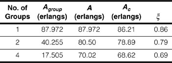
With a single group of 100 channels, each channel carries 86% of the load it could carry if it were continuously in use. When the pool of channels is subdivided into four groups, then to maintain a 2% GOS, each channel can carry only 69% of a full load.
Example
An AMPS system supports 395 voice channels per service block in each market area. For a seven-cell-cluster size, a cell can be assigned a maximum of 57 channels. As a complete pool, the 57 channels can support an offered load of A = 44.222 erlangs at a 1% blocking probability. The carried load is Ac = (1-0.01)44.222 = 43.78 erlangs, and the trunking efficiency is  , or 77%.
If 120°-sector antennas are used to improve the signal-to-interference ratio, then there will be 19 channels available in each sector. The offered load is now A = 3 x 11.230 = 33.69 erlangs (the offered load for one sector of 19 channels at 1% GOS is 11.230 erlangs, and there are three such sectors). The carried load is Ac = (1-0.01)33.69 = 33.35 erlangs, and the trunking efficiency is  , or 59%. The signal-to-interference ratio may be higher, but the amount of traffic that can be carried at the specified grade of service is substantially decreased.
The next example pulls together several ideas. It explores how system growth through sectoring is impacted by trunking efficiency considerations.
Example
A cellular system with an allocation of Nchan = 300 channels requires a 15 dB signal-to-interference ratio. A seven-cell-cluster layout with omnidirectional antennas has been performing adequately, but the system now needs additional channels to accommodate growth. An average subscriber places two calls per hour during the busy hour and holds each call an average of 3 min. Blocked calls are cleared, and the system offers a GOS of 5%. By what percentage can the number of subscribers be increased if 60° sectoring is introduced? The path-loss exponent is v = 4.
Solution
Let us begin by estimating the number of subscribers that a cell can support before sectoring. Each subscriber produces an offered load of Auser = 2 calls/60 min x 3 min = 0.1 erlang. For a seven-cell-cluster layout, the number of channels per cell is  . Using the Erlang B table in Appendix B with a GOS of 5% and 43 channels, we find that each cell can support a carried load of A = 37.565 erlangs. The number N of subscribers is then
  subscribers per cell.
We have encountered this sectoring problem previously as an example in the section titled "Sectoring." In that section we showed that using 60° sectors, the 15 dB signal-to-interference ratio could be maintained even if the cluster size is reduced to Kcluster = 4. Now with a reduced cluster size, the number of channels per cell is increased to  . Each cell is divided into six sectors, so the number of channels per sector is
  . From the Erlang B table with 12 channels we obtain (conservatively) Asector = 7.95 erlangs. Then for the entire cell, A = 6 x 7.95 = 47.7 erlangs. This gives a number of subscribers per cell of
  .
.
We now see that the number of subscribers has increased by  , or 27%. This is a substantial increase, but recall that the example in the "Sectoring" section showed an increase in the number Nmarket of channels of 75%. Counting the channels does not give a true picture of the increase in capacity, since dividing the cells into sectors causes a loss of trunking efficiency.
In this chapter we have focused on ways to design a wireless telecommunication system that will support a virtually unlimited number of users and span a virtually unlimited geographic range. We have shown that the frequency reuse concept arises as a natural solution in an environment in which the available radio spectrum is limited. We showed how a cellular organization provides a methodology for implementing frequency reuse. The following are the important ideas to take away as you conclude this chapter.
 , where v is the path-loss exponent. The cluster size must be large enough to ensure that the signal-to-interference ratio can produce an adequate quality of service.
Chapters 2, 3, and 4 have all been concerned with designing a communication system that can convey an amount of power between endpoints that is adequate to allow service. In Chapter 2 we investigated a point-to-point link in free space. In Chapter 3 we introduced real-world propagation conditions but continued our focus on a point-to-point link. In the present chapter we have shown how a single mobile switching center can communicate with a large number of users spread over a large geographic area. Conveying power, however, is not the same thing as conveying information. Establishing a power link is only a necessary first step. In the next few chapters we center our attention on methods of modulation and then characterize the information sources; that is, we will be concerned with techniques for conveying information over the power link that we have established.
The first FCC spectrum allocation for cellular mobile telephone service consisted of two bands totaling 40 MHz. The upper band, 870–890 MHz, was reserved for forward channels or downlink transmissions, and the lower band, 825–845 MHz, was reserved for reverse channels or uplink transmissions. Forward channels are those used for transmissions from a base station to a mobile unit, and reverse channels are those used for transmissions from a mobile unit to a base station. The first cellular systems were designed for telephone (voice) services only and required two 30 kHz channels for a single two-way telephone call.
A. How many complete channel pairs were allocated?
B. The FCC specified that channels be numbered sequentially with reverse channel 1 located at 825.030 MHz and forward channel 1 located at 870.030 MHz. Write a simple expression that specifies the channel center frequency given the channel number for both forward and reverse channels.
C. In 1989 an additional allocation of 10 MHz (5 MHz for each direction) was made as follows: 824–825 MHz and 845–849 MHz for reverse channels, and 869–870 MHz and 890–894 MHz for forward channels. How many additional channel pairs did this allocation provide, and what is the total number of channel pairs available in the augmented cellular band?
D. The channel numbers for the 845–849 MHz (and 890–894 MHz) band are a continuation of those in the original allocation. To simplify digital logic computation, however, the channel numbers in the 824–825 MHz band are represented as the decimal equivalent of the 9-bit two's complement of negative channel numbers starting at channel 0. For example, channel 0 is represented as 111111111, which is 1023 in decimal, and channel 1 is 11111110, which is 1022 in decimal. What are the channel numbers for the channel pairs in the lower 1 MHz bands? Write expressions for the channel center frequencies of the 824–825 MHz and 869–870 MHz band channels.
Consider a linear arrangement of base stations as shown in Figure P 4.1. Each base station is separated from its nearest neighbor by a distance 2R, where R is the radius of the circular coverage area (cell) for each base station. Apart from the transmission frequency, assume that all base stations are identical and that the environment is uniform with path loss of v. Assume that the mobile unit (MU) is located at the edge of the serving cell, that is, the area covered by BS0. Assume that the nearest or first-tier cochannel neighbors are BS-k and BSk, and the reuse distance is denoted as D. (The figure shows the special case D = 2.)
Figure P 4.1. Linear Arrangement of Cells
A. Write an expression for the frequency reuse ratio Q as a function of k.
B. Write a general expression for the S/I at the mobile unit from its first-tier cochannel neighbors (interference sources) as a function of k and v.
For the system in Problem 4.2, compute the S/I in decibels from the first-tier interference sources located at BS-3 and BS3 for a path loss of v = 3. For this case, how does the S/I degrade if we include second-tier interference, that is, interference from BS-6 and BS6?
For the initial 40 MHz spectrum allocation for cellular mobile telephones and the system of cells described in Problem 4.2, how many channel sets and how many complete channel pairs per set would be deployed for a reuse factor Q of 6?
For the FCC spectrum allocation described in Problem 4.1, channels are separated by 30 kHz. For any channel i, the channels i + 1 and i - 1 are defined as the adjacent channels of channel i. In the absence of ideal or very sharp cutoff filters in the receiver, any channel i is subject to interference from its neighboring or adjacent channels. For example, a BS receiver operating on channel i will also receive signal energy from MUs operating on channels i - 1 and i + 1. The adjacent channel signal level, however, will be attenuated, depending on the out-of-band characteristics of the receiver filter. Assume that the adjacent-channel signal power is attenuated by a factor α after filtering and that all MUs transmit at the same power level. (Note: a similar situation exists for adjacent-channel BS transmissions.)
A. Define a scheme for deploying radio channels for the system of Problem 4.3 so as to minimize the effects of adjacent-channel interference.
B. For this deployment and a worst-case situation, write an expression for the power level of adjacent-channel interference relative to the serving signal power at an MU after filtering.
Write an expression for the worst-case signal-to-adjacent-channel-interference ratio at the output of the receiver filter at BS0 on channel 4, when interference comes from MUs being served on channels 3 and 5 in BS-1 and BS1 respectively.
Assuming that the coverage from any given BS is circular, calculate the percentage overlap when cell BSs are deployed on a triangular, rectangular, and hexagonal grid. See Figure 4.4 and Figure 4.5.
What is the smallest reuse distance that can be used to ensure a 20 dB S/I ratio at a cell boundary when the path-loss exponent is v = 3.2? How many cells are in a cluster for this reuse distance?
A certain metropolitan area covers 400 mi2.
A. What is the minimum number of 1.5 mi cells required to provide radio coverage for the entire metropolitan area?
B. If the path-loss exponent v is 3.5, what is the minimum cluster size that will ensure a 15 dB S/I at the cell boundary?
C. If there are 490 channels allocated to provide the service, how many channels are available in each cell and how many channels are available to serve users?
Extend Table 4.2 to provide values of S/I|dB for path-loss exponents v = 3.5 and v = 3, and plot S/I|dB versus Q, the reuse ratio, for each path-loss exponent, that is, 3, 3.5, and 4. Describe how path loss affects reuse, and discuss the ramifications to coverage and capacity. If you were designing a system for a given area, what would you need to know about the area and how would that information influence your cell parameters and layout? Assume that a large number of channels, Nchan, is available.
The radio resource density (or simply the radio density), ρ, is an interesting parameter that relates to the system's capacity to serve users simultaneously. The radio density is simply the number of radios per unit area. Develop an expression for ρ in terms of the reuse ratio Q, the cell area Acell, and the number Nchan of channels.
The most expensive element in the deployment of a wireless system is the set of BSs and associated real estate. Assume that a metropolitan region of area Asys is to be covered by a system allocated Nchan channels.
A. Given the path-loss exponent v, develop an approximate relationship for the total cost CT of the BSs as a function of the radio density ρ, QoS objective in the form of the minimum S/I, and the cost per BS CBS. (Note: The approximation comes about in using the relationship for S/I.)
B. For a uniform deployment of cells, discuss how the total cost of BSs is affected by the spectrum allocation, radio density, and QoS.
C. How does the path-loss exponent v affect the radio density?
For a path-loss exponent v = 4, compute S/I|dB for a reuse (cluster size) of seven including first- and second-tier interference sources. How much does the S/I|dB degrade when third-tier interference sources are included?
The approximation for S/I resulting from first-tier cochannel interferers, that is,  , is poorest for small reuse ratios. Write an exact expression for the S/I resulting from first-tier cochannel interferers for a reuse of 1, and compute the S/I|dB for a path-loss exponent v = 4. Compare your answer with the result contained in Table 4.2.
For a certain deployment, suppose that adjacent channels are deployed only at adjacent BSs. Assuming that all BSs are identical, how much attenuation (in decibels) is required for an MU receiver filter to ensure a 40 dB margin against adjacent-channel interference in the worst case?
First-generation and most second-generation cellular systems relied on the geographic separation of cochannel radios to achieve a given S/I and therefore a given quality of service. Given the minimum required S/I, however, the reuse ratio and cluster size are determined. System capacity is related to reuse (cluster size) and is a maximum for a reuse of 1; however, the S/I ratio is minimized for a reuse of 1.
Suppose that a system could be devised so that the signal could be enhanced relative to the interference using signal processing. Indeed, such a system exists, and it uses a technique termed code-division multiple access (CDMA). If such a system were used, what is the processing gain it must provide in order to achieve an effective 17 dB S/I ratio for a reuse of 1 and uniform path-loss exponent v = 4? Consider both first- and second-tier cochannel interference sources, and use an exact formulation for the first tier.
In the ideal case, sectorization reduces cochannel interference by eliminating the interference from four of the six first-tier interferers. Realizable sectored antennas, however, do receive (and transmit) some energy outside the sector main lobe. Assume that the gain outside the main lobe is a uniform 30 dB down from the peak gain of the main lobe. Calculate the worst-case S/I ratio (first-tier interference solutions only) for v = 4 and a cluster size of seven. How does this compare to the cases of ideal sectored antennas and omnidirectional antennas?
Using the results of Problem 4.16, determine how 120° sectorization improves S/I|dB for a system of reuse of 1. Consider both first- and second-tier interference solutions.
Draw and label a 12-cell cluster. Assume that all cells in this cluster are to be split and overlaid with half-radius cells. Draw and label all the half-radius (split) cells necessary to completely cover the original 12-cell cluster. Assume that each of the original cells has a base station at its center and that these base stations will be reused after the split.
Assume that average users place two calls of 15 min duration per hour in a given system.
A. Given a seven-cell reuse (cluster size), compute the carried load per cell and trunking efficiency for a 2% GOS and 665-channel allocation.
B. Calculate the number of users that can be accommodated in each cell at the given GOS.
C. Compute the carried load and trunking efficiency if the reuse for the same seven cells were reduced to one.