Each of the three topics discussed in this chapter appears only on the BC exam. If you’re in an AB course, move on to Chapter 21.
Another way to apply integrals is to find the length of the graph. It’s usually a pretty simple problem. All you have to do is use a formula.
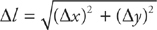
Suppose you want to find the length of the graph of a function y = f(x) from x = a to x = b. Call this length L. You could divide L into a set of line segments, ∆l, add up the lengths of each of them, and you would find L. The formula for the length of each line segment can be found with the Pythagorean theorem:
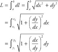
If we make ∆l, ∆x, and ∆y infinitesimally small, they become dl, dx and dy. If we then add up all of these line segments, we get:
Here’s the rule:
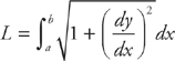
If the function f(x) is continuous and differentiable on [a, b], then the length of the curve y = f(x) from a to b is:
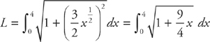
Example 1: Find the length of the curve  from x = 0 to x = 4.
First, find the first derivative of the function:  .
.
Next, plug into the formula:

Now evaluate the integral:
Using u-substitution, let 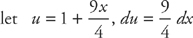 , and
, and  . Then substitute:

Once you substitute back, the result is: 
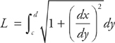
Sometimes you’ll be given the curve as a function of y instead of as a function of x. Then the formula for the length of the curve x = f(y) on the interval [c, d] is:
Example 2: Find the length of the curve x = sin y, from y = 0 to y =  . Set up but do not evaluate the integral.
Since  = cos y, we can plug it into the formula:
 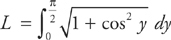 .
.
Sometimes the curve will be defined parametrically, usually in terms of t (for time). Then the formula for the length of the curve from t = a to t = b is:
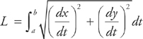
Example 3: Find the length of the curve defined by x = sin t and y = cos t, from t = 0 to t = π.
Take the derivatives of the two t-functions:  = cos t and
  = − sin t Then use the formula:

If you evaluate the integral, you get:

That’s all there is to finding the length of a curve. As you’ve seen, many applications of the integral involve simple formulas. All you have to do is to plug in and evaluate the integral. If the integral is a difficult one, you probably just have to set it up.
Try these solved problems. Do each problem, covering the answer first, then check your answer.
PROBLEM 1. Find the length of the curve  from x = 0 to x = 3.
Answer: First, we find the first derivative 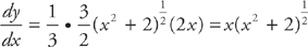
Next, plug into the formula:

Now you just have to evaluate the integral:

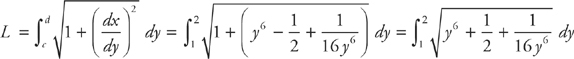
PROBLEM 2. Find the length of the curve  from y = 1 to y = 2.
Answer: Here, you have x in terms of y, so first we find :

Next, find  :
:

Plug this into the formula:
And evaluate the integral:

PROBLEM 3. Find the length of the curve x = tan t and y = sec t from t = 0 to t =  . Set up but do not evaluate the integral.
Answer:

To use the above formula, you need to determine that = sec2 t and sec t tan t. Plug these into the formula:

Find the length of the following curves between the specified intervals. Evaluate the integrals unless the directions state otherwise. The answers are in Chapter 23.
1.  from x = 1 to x = 2
2. y = tan x from x = − to x = 0 (Set up but do not evaluate the integral.)
3.  from x = 0 to x =
  (Set up but do not evaluate the integral.)
4.  from y = 2 to y = 3
5.  from y = −
  to y = (Set up but do not evaluate the integral.)
6. x = sin y – y cos y from y = 0 to y = π (Set up but do not evaluate the integral.)
7. x = cos t and y = sin t from t = to t = 
8. x =  and
and  from t = 1 to t = 4 (Set up but do not evaluate the integral.)
9. x = 3t2 and y = 2t from t = 1 to t = 2 (Set up but do not evaluate the integral.)
This is the last technique you’ll learn to evaluate integrals. There are many, many more types of integrals and techniques to learn; in fact, there are courses in college primarily concerned with integrals and their uses! Fortunately for you, they’re not on the AP exam (and therefore, not in this book). The BC exam usually has a partial fractions integral or two, and the concept isn’t terribly hard.
We use the method of partial fractions to evaluate certain types of integrals that contain rational expressions. First, let’s discuss the type of algebra you’ll be doing.
If you wanted to add the expressions  and
and  , you would do the following:
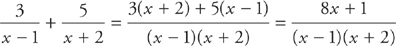
Now, suppose you had to do this in reverse; you were given the fraction on the right and you wanted to determine what two fractions were added to give you that fraction. Another way of asking this is: What constants A and B exist, such that 
How do you go about solving for A and B? First, multiply through by (x – 1)(x + 2) to clear the denominator:
A(x + 2) + B(x – 1) = 8x + 1
Next, simplify the left side:
Ax + 2A + Bx – B = 8x + 1
Now, if you group the terms on the left, you get:
(A + B)x + (2A – B) = 8x + 1
Therefore, A + B = 8 and 2A – B = 1
If you solve this pair of simultaneous equations, you get A = 3 and B = 5. Surprised? We hope not.
Why would you need to know this method? Suppose you wanted to find:

You now know you can rewrite this integral as:

These integrals are easily evaluated:

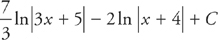
Example 1: Evaluate  .
.
You need to find A and B such that:

First, multiply through by (3x + 5)(x + 4):
A(x + 4) + B(3x + 5) = x + 18
Next, simplify and group the terms:
Ax + 4A + 3Bx + 5B = x + 18
(A + 3B)x + (4A + 5B) = x + 18
You now have two simultaneous equations: A + 3B = 1 and 4A + 5B = 18. If we solve the equations, we get A = 7 and B = –2. Thus, you can rewrite the integral as:
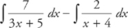
These are both logarithmic integrals. The solution is:
There are three main types of partial fractions that appear on the AP exam. You’ve just seen the first type: one with two linear factors in the denominator. The second type has a repeated linear term in the denominator.
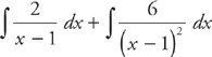
Example 2: Evaluate  .
.
Now you need to find two constants A and B, such that:

Multiplying through by (x – 1)2, we get: A(x – 1) + B = 2x + 4. Now simplify:
Ax – A + B = 2x + 4
Ax + (B – A) = 2x + 4
Thus, A = 2 and B – A = 4, so B = 6. Now we can rewrite the integral as:
The solution is:

The third type has an irreducible quadratic factor in the denominator.
Example 3: Evaluate 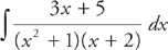 .
.
For a quadratic factor, you need to find A, B, and C such that:

Now you have a term Ax + B over the quadratic term. Whenever you have a quadratic factor, you need to use a linear numerator, not a constant numerator.
Multiply through by (x2 + 1)(x + 2) and you get:
(Ax + B)(x + 2) + C(x2 + 1) = 3x + 5
Simplify and group the terms:
Ax2 + 2Ax + Bx + 2B + Cx2 + C = 3x + 5
(A + C)x2 + (2A + B)x + (2B + C) = 3x + 5
This gives you three equations:
A + C = 0
2A + B = 3
2B + C = 5
If you solve these three equations, the values are:

Now you can rewrite the integral:
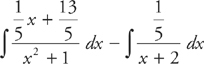
Break the first integral into two integrals:
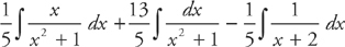
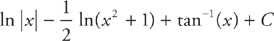
You can evaluate the first integral using u-substitution; the second integral is inverse tangent, and the third integral is a natural logarithm:

Notice how all of these integrals contained a natural logarithm term? That’s typical of a partial fractions integral. Now try these solved problems. Do each problem, covering the answer first, then check your answer.
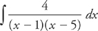
PROBLEM 1. Evaluate  .
.
Answer: First, factor the denominator:
Find A and B such that:
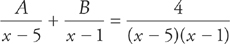
First, multiply through by (x – 5)(x – 1):
A(x – 1) + B(x – 5) = 4
Next, simplify and group the terms:
Ax – A + Bx – 5B = 4
(A + B)x + (–A – 5B) = 4
You now have two simultaneous equations: A + B = 0 and –A – 5B = 4. If you solve the equations, you get A = 1 and B = –1. Thus, we can rewrite the integral as:
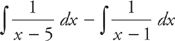
These are both logarithmic integrals. The solution is: ln|x – 5| – ln|x – 1| + C.
Answer: You need to find A, B, and C, such that:

Multiply through by x(x2 + 1):
A(x2 + 1) + (Bx + C)(x) = x + 1
Simplify and group the terms:
Ax2 + A + Bx2 + Cx = x + 1
(A + B)x2 + Cx + A = x + 1
Now you have three equations:
A + B = 0
C = 1
A = 1
You have to solve only for B: Since A = 1, B = –1. Now rewrite the integral as:

Break this into:
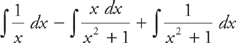
The first integral is a natural logarithm, the second integral requires u-substitution, and the third integral is an inverse tangent. The answer is:
Evaluate the following integrals. The answers are in Chapter 23.
There’s one last type of integral that shows up on the BC exam. These are improper integrals, which are integrals evaluated over an open interval, rather than a closed one. More formally, an integral is improper if: (a) its integrand becomes infinite at one or more points in the interval of integration; or (b) one or both of the limits of integration is infinite.
We integrate an improper integral by evaluating the integral for a constant (a) and then taking the limit of the resulting integral as a approaches the limit in question. If the limit exists, the integral converges and the value of the integral is the limit. If the limit doesn’t exist, the integral diverges and the integral cannot be evaluated there.
Confusing, huh? Let’s clear the air with an example.
Example 1: Evaluate  .
.
At x = 4, the denominator is zero and the integrand is undefined. Therefore, replace the 4 in the limit of the integral with a and evaluate:

Multiply the numerator and the denominator of the integrand by  :
:
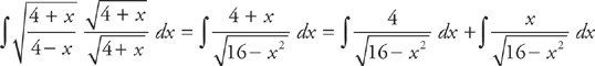
Evaluate the first integral by factoring 16 out of the denominator:

Next, use u-substitution. Let u =  and du = dx:

Evaluate the second integral with u-substitution. Let u = 16 – x2 and du = –2x dx:

The final result is:

Now you have to evaluate the integral at the limits of integration:
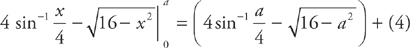
Finally, take the limit as a approaches 4:

This may look complicated, but it was actually a very straightforward process. Because the integrand didn’t exist at x = 4, replace 4 with a and then integrate. When you evaluated the limits of integration using a instead of 4, you then took the limit as a approaches 4.
Example 2: Evaluate  .
.
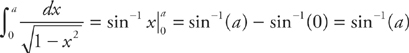
Replace the upper limit of integration with a and take the limit as a approaches infinity:

Integrate:
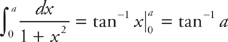
Now, take the limit:

Let’s do an integral that becomes undefined in the middle of the limits of integration.
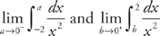
Example 3: Evaluate  .
.
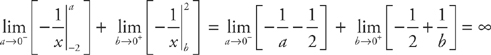
Note that this integral becomes undefined at x = 1. Because of this, you have to divide the integral into two parts: one for x < 1 and one for x > 1:
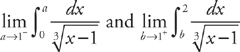
If either of these limits fails to exist, then the integral from 0 to 2 diverges. Evaluate them both:
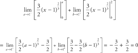
Because both limits exist and are finite, the integral converges and the value is 0.
There are several other facets of evaluating improper integrals that we won’t explore here because they don’t appear on the AP exam. You’ll have to do only the most simple of these, usually one with infinity as a limit of integration.
Evaluate these integrals and check your work.
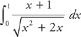
PROBLEM 1. Evaluate  .
.
Answer: First, evaluate the integral:

Next, we evaluate the limit: 
Therefore  , and the integral diverges.
Answer: Evaluate the integral:

Next, evaluate the limit:

Therefore  , and the integral converges.
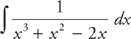
PROBLEM 3. Evaluate  .
.
Answer: Evaluate the integral:
Next evaluate:

Therefore 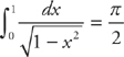 , and the integral converges.
PROBLEM 4. Evaluate  .
.
Answer: The integrand becomes undefined at x = 0, so you have to divide the integral into:
Now, evaluating both integrals:
The integral diverges.
Evaluate the following integrals. The answers are in Chapter 23.
The topic of polar curves usually shows up as only one multiple-choice problem on the BC exam. However, we will cover the two most typical aspects of the calculus of polar curves. We expect that you had a full treatment of polar coordinates and curves in precalculus, so we won’t cover them here.
The slope of a polar curve r = f(θ) is  . Because x and y are defined parametrically, we need to derive in terms of r and θ. Remember that in polar coordinates, x = r cos θ = f(θ) cos θ and y = r sin θ = f(θ) sin θ.
Note that: 
We substitute for x and y: 
Using the Product Rule, we get: 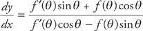
This is the formula for finding the slope of a polar curve r = f(θ).
Example 1: Find the slope of the tangent line to the curve r = 2 + 4 sin θ.
First, let’s find f′(θ): f′(θ) = 4 cos θ
This gives us:

We are not going to derive the formula for you. If we want to find the area of a region between the origin and the curve r = f(θ), a ≤ θ ≤ b, we use the formula:  .
.
Example 2: Find the area of the region in the plane enclosed by the cardioid r = 4 + 4sinθ.
First, let’s graph the curve:
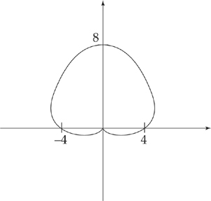
Because r sweeps out the region as θ goes from 0 to 2π, these are our limits of integration.
Plug into the formula for area:

Evaluate the integral:

Use the trig identity 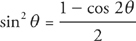 to rewrite the integrand:

Evaluate the integral:

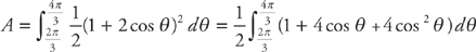
Example 3: Find the area inside the smaller loop of the limaçon: r = 1 + 2 cos θ.
First, let’s graph the curve:

Because in the inner loop, r sweeps out the region as θ goes from  to
to  , these are our limits of integration.
Plug into the formula for area:

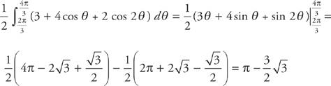
Evaluate the integral:
Use the trig identity  to rewrite the integrand:

Evaluate the integral:
Again, we are not going to derive the formula for you. If we want to find the area of a region between the curves r1 = f1(θ) and r2 = f2(θ), with 0 ≤ r1(θ) ≤ r2(θ) and a ≤ θ ≤ b, we use the formula:  .
.
Example 4: Find the area of the region inside the circle r = 4 and outside r = 4 – cosθ.
First, let’s graph the region:

Because r sweeps out the region as θ goes from – to , these are our limits of integration. Here, because of symmetry, instead of evaluating 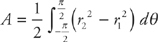 , we can evaluate
 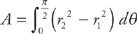 .
.
Plug into the formula for area:

Use the trig identity  to rewrite the integrand:

Evaluate the integral:

Do the following problems on your own. The answers are in Chapter 23.
1. Find the slope of the curve r = 2 cos 4θ.
2. Find the slope of the curve r = 2 – 3 sin θ at (2, π).
3. Find the area inside the limaçon r = 4 + 2 cos θ.
4. Find the area inside one loop of the lemniscate r2 = 4 cos 2θ.
5. Find the area inside r = 2 cos θ and outside r = 1.
6. Find the area inside the lemniscate r2 = 6 cos 2θ and outside the circle r =  .
.
 .
.


 .
.