
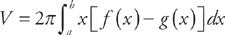
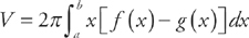
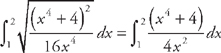
We find the area of a region bounded by f(x) above and g(x) below at all points of the interval [a, b] using the formula  . Here, f(x) = 2 and g(x) = x2 – 2. First, let’s make a sketch of the region:
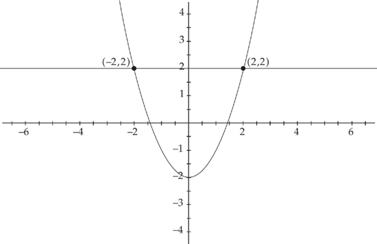
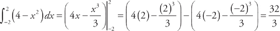
Next, we need to find where the two curves intersect, which will be the endpoints of the region. We do this by setting the two curves equal to each other. We get: x2 – 2 = 2. The solutions are (–2,0) and (2,0). Therefore, in order to find the area of the region, we need to evaluate the integral  . We get:
 .
.

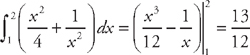
We find the area of a region bounded by f(x) above and g(x) below at all points of the interval [a,b] using the formula  . Here, f(x) = 4x – x2 and g(x) = x2.
First, let’s make a sketch of the region:
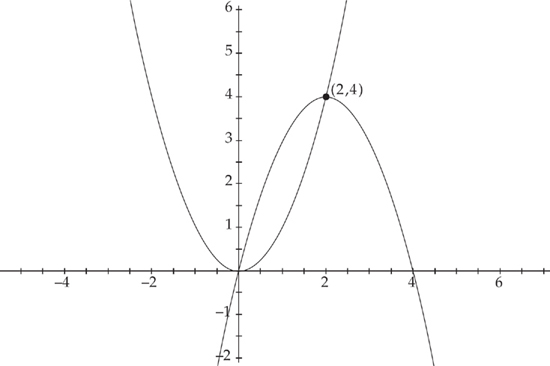
Next, we need to find where the two curves intersect, which will be the endpoints of the region. We do this by setting the two curves equal to each other. We get: 4x – x2 = x2. The solutions are (0,0) and (2,4). Therefore, in order to find the area of the region, we need to evaluate the integral 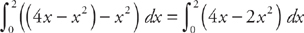 . We get:
  .
.

We find the area of a region bounded by f(x) above and g(x) below at all points of the interval [a, b] using the formula  . Here, f(x) = x3 and g(x) = 3x2 – 4.
First, let’s make a sketch of the region:
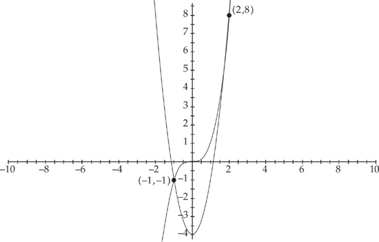
Next, we need to find where the two curves intersect, which will be the endpoints of the region. We do this by setting the two curves equal to each other. We get: 3x2 – 4 = x3. The solutions are (–1, –1) and (2, 8). Therefore, in order to find the area of the region, we need to evaluate the integral  . We get:
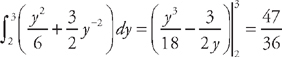
4. 36
We find the area of a region bounded by f(x) above and g(x) below at all points of the interval [a, b] using the formula  . Here, f(x) = 2x – 5 and g(x) = x2 – 4x – 5.
First, let’s make a sketch of the region:

Next, we need to find where the two curves intersect, which will be the endpoints of the region. We do this by setting the two curves equal to each other. We get: x2 – 4x – 5 = 2x – 5. The solutions are (0,–5) and (6,7). Therefore, in order to find the area of the region, we need to evaluate the integral  . We get:
 .
.
We find the area of a region bounded by f(x) above and g(x) below at all points of the interval [a, b] using the formula 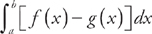 .
.
First, let’s make a sketch of the region:
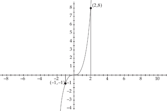
Notice that in the region from x = –1 to x = 0 the top curve is f(x) = 0 (the x‑axis) and the bottom curve is g(x) = x3, but from x = 0 to x = 2 the situation is reversed, so the top curve is f(x) = x3 and the bottom curve is g(x) = 0. Thus, we split the region into two pieces and find the area by evaluating two integrals and adding the answers: 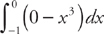 and
and  . We get:
  and
and  . Therefore, the area of the region is
  .
.

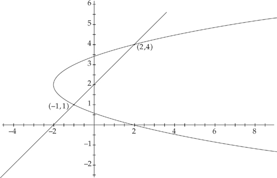
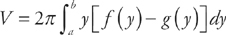
We find the area of a region bounded by f(y) on the right and g(y) on the left at all points of the interval [c, d] using the formula  . Here, f(y) = y + 2 and g(y) = y2.
First, let’s make a sketch of the region:
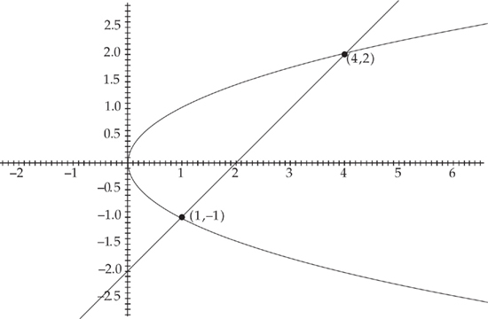
Next, we need to find where the two curves intersect, which will be the endpoints of the region. We do this by setting the two curves equal to each other. We get: y2 = y + 2. The solutions are (4,2) and (1,–1). Therefore, in order to find the area of the region, we need to evaluate the integral 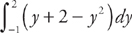 . We get:

7. 4
We find the area of a region bounded by f(y) on the right and g(y) on the left at all points of the interval [c, d] using the formula  . Here, f(y) = 3 – 2y2 and g(y) = y2.
First, let’s make a sketch of the region:
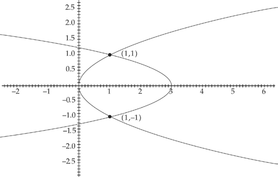
Next, we need to find where the two curves intersect, which will be the endpoints of the region. We do this by setting the two curves equal to each other. We get: y2 = 3 – 2y2. The solutions are (1,1) and (1, –1). Therefore, in order to find the area of the region, we need to evaluate the integral  . We get:
  .
.

We find the area of a region bounded by f(y) on the right and g(y) on the left at all points of the interval [c, d] using the formula  . Here, f(y) = y3 – y2 and g(y) = 2y.
First, let’s make a sketch of the region:
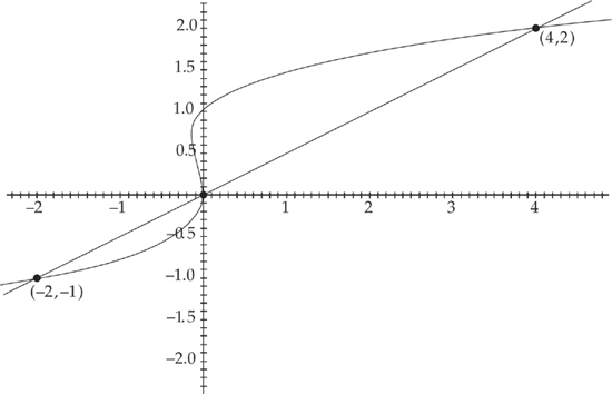
Next, we need to find where the two curves intersect, which will be the endpoints of the region. We do this by setting the two curves equal to each other. We get: y3 – y2 = 2y. The solutions are (4,2), (0,0) and (–2,–1). Notice that in the region from y = –1 to y = 0, the right curve is f(y) = y3 – y2 and the left curve is g(y) = 2y, but from y = 0 to y = 2 the situation is reversed, so the right curve is f(y) = 2y and the left curve is g(y) = y3 – y2. Thus, we split the region into two pieces and find the area by evaluating two integrals and adding the answers:  and
and  . We get:
  and
and  . Therefore, the area of the region is
  .
.
We find the area of a region bounded by f(y) on the right and g(y) on the left at all points of the interval [c, d] using the formula 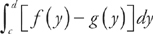 . Here, f(y) = y – 2 and g(y) = y2 – 4y + 2. First, let’s make a sketch of the region:
Next, we need to find where the two curves intersect, which will be the endpoints of the region. We do this by setting the two curves equal to each other. We get: y2 – 4y + 2 = y – 2. The solutions are (2,4) and (–1,1). Therefore, in order to find the area of the region, we need to evaluate the integral  . We get:

We find the area of a region bounded by f(y) on the right and g(y) on the left at all points of the interval [c, d] using the formula 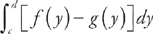 . Here, f(y) = 2 – y4 and
  . First, let’s make a sketch of the region:
Next, we need to find where the two curves intersect, which will be the endpoints of the region. We do this by setting the two curves equal to each other. We get:  . The solutions are (1,1) and (1,–1). Therefore, in order to find the area of the region, we need to evaluate the integral
  . We get:
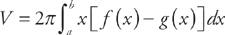
 (see
(see  and the x-axis. First, we need to find the endpoints of the region. We do this by setting
  equal to zero and solving for x. We get: x = –3 and x = 3. Thus, we will find the volume by evaluating
  . We get:
 (see
(see  and
and  . Thus, we will find the volume by evaluating
  . We get:
 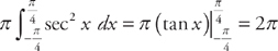 .
.
 (see
(see 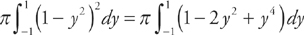 . We get:
  .
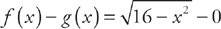
. (see
(see  and the y-axis. We are given the endpoints of the region: y = –1 and y = 1. Thus, we will find the volume by evaluating
  . We get:
 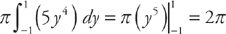 .
.
 (see
(see 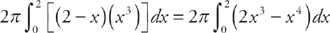 . We get:
 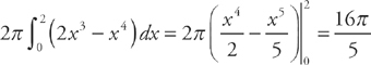 .
. (see
(see  . Thus, the height of each shell is
  and the radius is simply x. The endpoints of our region are x = 0 and x = 2. Therefore, we will find the volume by evaluating:
 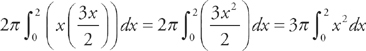 . We get:
 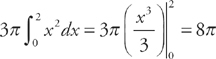 .
.
 (see
(see  and g(x) = 2x – 1. Thus, the height of each shell is
  and the radius is simply x. The left endpoint of our region is x = 0 and we find the right endpoint by finding where f(x) =
  . We get:
 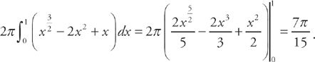 .
.
 (see
(see  (which we get by solving y = x2 for x) and g(y) = 0 (the y-axis). We can easily see that the top endpoint is y = 4 and the bottom one is y = 0. Therefore, we will find the volume by evaluating:
 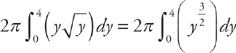 . We get:
 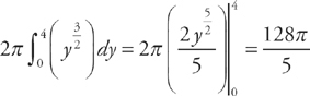 .
.
 (see
(see  . We get:
 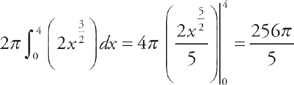 .
.
 (see
(see  (which we get by solving y2 = 8x for y and taking the top half above the x-axis) and
  (the bottom half). Thus the height of each shell is
  . We can easily see that the left endpoint is x = 0 and that the right endpoint is x = 2. Next, note that we are not revolving around the x-axis but around the line x = 4. Thus, the radius of each shell is not x but rather 4 – x. Therefore, we will find the volume by evaluating:
 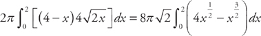 . We get:
 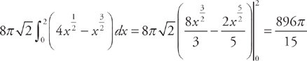 .
.
 and the intervals are found by setting
 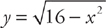 equal to zero. We get: x = –4 and x = 4. Thus, we find the volume by evaluating the integral
 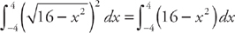 . We get:
  .
.
 over the endpoints of the interval. Here, the hypotenuses of the triangles are found by f(x) – g(x) = 4 – x2 and the intervals are found by setting y = x2 equal to y = 4. We get: x = –2 and x = 2. Thus, we find the volume by evaluating the integral
 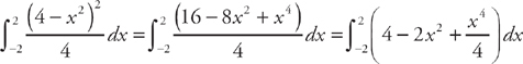 . We get:
  .
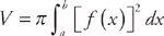
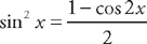
. , where both u and v are functions of x. The formula for evaluating the integral is:
 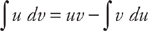 (see
(see  . Plugging into the formula, we get:
  . Now we just have to find
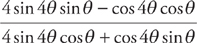
  . We do this by rewriting the integrand in terms of sin x and cos x:
  . Therefore,
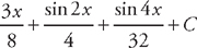
  .
.
 , where both u and v are functions of x. The formula for evaluating the integral is:
  (see
(see 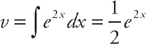 . Plugging into the formula, we get:
  . Now we just have to find
  :
:  . Therefore,
 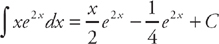 .
.
 , where both u and v are functions of x. The formula for evaluating the integral is:
  (see
(see  , then we can find du by taking the derivative of u, and we can find v by taking the integral of dv. We get:
  and
and  . Plugging into the formula, we get:
  . Now we just have to find
  . Therefore,
  .
. , where both u and v are functions of x. The formula for evaluating the integral is:
  (see
(see  . Plugging into the formula, we get:
 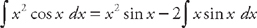 . Now we have to find
  . Once again we will have to use integration by parts. This time, if we let u = x and dv = sin x dx, then du = dx and
  . Plugging into the formula, we get:
 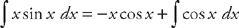 . Finally, we have to find
  . Putting everything together, we get:
  .
.
 , where both u and v are functions of x. The formula for evaluating the integral is:
  (see
(see  and
and 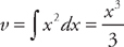 . Plugging into the formula, we get:
  . Now we just have to find
  . Therefore,
  .
.
 , where both u and v are functions of x. The formula for evaluating the integral is:
  (see
(see 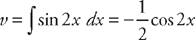 . Plugging into the formula, we get:
  . Now we just have to find
  . Therefore,
  .
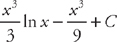
. , where both u and v are functions of x. The formula for evaluating the integral is:
 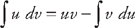 (see
(see  and
and  . Plugging into the formula, we get:
  . Now we have to find
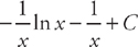
  . Once again we will have to use integration by parts. This time, if we let u = ln x and dv = dx, then
  and
and  . Plugging into the formula, we get:
 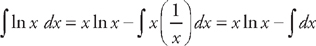 . Finally we have to find
  . Putting everything together, we get:
  .
. , where both u and v are functions of x. The formula for evaluating the integral is:
 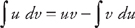 (see
(see  . Plugging into the formula, we get:
 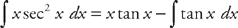 . Now we just have to find
  . We do this by rewriting the integrand in terms of sin x and cos x:
 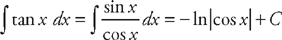 . Therefore,
 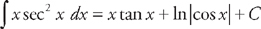 .
.
 (see
(see  , so
, so  . Therefore,
 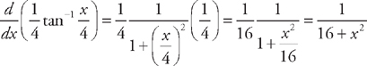 .
.
 (see
(see  , so
, so  . Therefore,
  .
.
 (see
(see  . Therefore,
 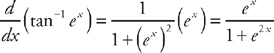 .
.
 (see
(see  and we just need to rearrange the integrand so that it is in the proper form to use the integral formula. If we factor
 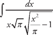 . Next, we do u-substitution. Let
  and
and  . Multiply both by
  so that
  and
and  . Substituting into the integrand we get:
 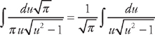 . Now we get:
 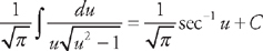 . Substituting back we get:
  .
.
 (see
(see  and we just need to rearrange the integrand so that it is in the proper form to use the integral formula. If we factor 7 out of the denominator we get:
  . Next, we do u-substitution. Let
  and
and  . Multiply du by
  so that
  . Substituting into the integrand we get:
  . Now we get:
  . Substituting back we get:
  .
. (see
(see  and we will need to do u-substitution. Let u = ln x and
  . Substituting into the integrand we get:
  . Substituting back we get: tan–1(ln x) + C.
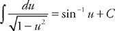 (see
(see  and we will need to do u-substitution. Let u = tan x and du = sec2 x dx. Substituting into the integrand we get:
  . Substituting back we get: sin–1(tan x) + C.
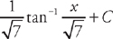
 (see
(see  and we just need to rearrange the integrand so that it is in the proper form to use the integral formula. If we factor 9 out of the radicand we get:
 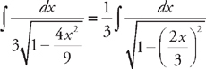 . Next, we do u-substitution. Let
  and
and  . Multiply du by
  so that
  . Substituting back we get:
  .
.
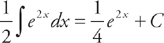
 (see
(see  and we will need to do u-substitution. Let u = e3x and du = 3e3x dx. Divide du by 3 so that
  . Substituting into the integrand we get:
  . Substituting back we get:
  .
.
 into the integrand. We get:
 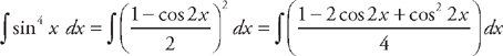 . We can break this into three integrals:
  . The first two integrals are easy:
  . For the third integral, we use the substitution
 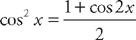 . We get:
  . Now we integrate these:
 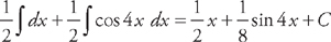 . Now we put everything together to get:
 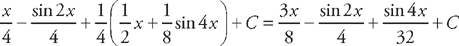 .
.
 into the integrand. We get:
 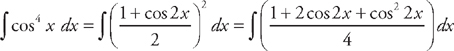 . We can break this into three integrals:
  . The first two integrals are easy:
 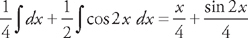 . For the third integral, we again use the substitution
  . We get:
 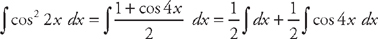 . Now we integrate these:
 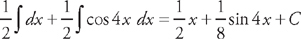 . Now we put everything together to get:
 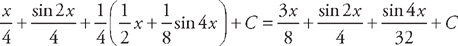 .
.
 . Now we substitute back:
 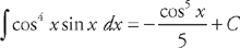 .
.
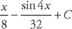
 . Next, we use the trig identity sin2 x = 1 – cos2 x and substitute into the integrand:
 . Now we can use u‑substitution.
 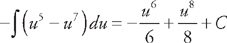 . Now we substitute back:
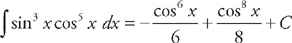 .
.
 . Next, we use the substitution
  into the integrand:
  . We use a little algebra:
 . The first integral is easy:
  . For the second integral, we again use the substitution
  into the integrand:
 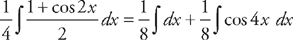 . These are both easy to integrate:
 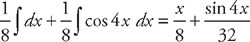 . Putting it all together, we get:
  .
. . Now, we can use the substitution
  to rewrite the integrand:
 . This is easy to integrate:
  . This is why you should know your trigonometric identities really well before you take calculus!
 . Now we substitute back:
 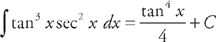 .
.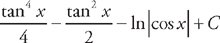
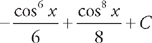
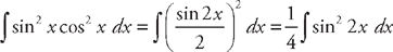
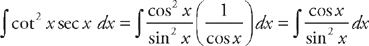
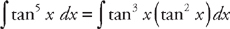 . Next, we use the trigonometric identity tan2 x = sec2 x – 1 and rewrite the integrand:
  . Now we break this into two integrals:
  . Next, break up the integrand of the second integral into
 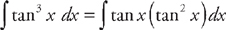 . Once again, use the trigonometric identity tan2 x = sec2 x – 1 to rewrite the integrand:
  . Putting the integrals
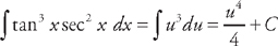
  . We can use u-substitution to find the first two integrals. If we let u = tan x, then du = sec2 x dx. Substituting into the integrand, we get:
  . Substituting back, we get:
 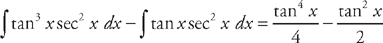 . The last integral we have done before (see
 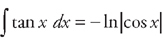 . Therefore
  .
. . Next, we do u‑substitution. If we let u = sin x, then du = cos x dx. Substituting into the integrand, we get:
  . Substituting back, we get:
 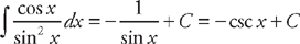 .
.
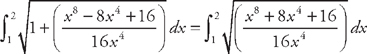
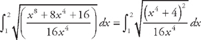
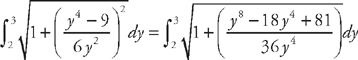
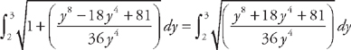
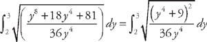
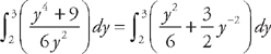
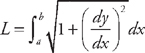 (see
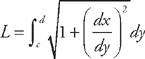
(see  from x = 1 to x = 2. First, we need to find the derivative:
  . Now we plug this into the formula for the length:
 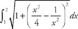 . Now we need to use
 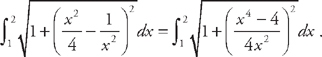 .
. .
. .
. .
. .
. .
. .
.
 (see
(see  to x = 0. First, we need to find the derivative:
  . Now we plug this into the formula for the length:
 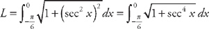 .
.
 (see
(see  from x = 0 to x =
  . First, we need to find the derivative:
  . Now we plug this into the formula for the length:
  .
.
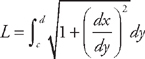 (see
(see  from y = 2 to y = 3. First, we need to find the derivative:
 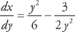 . Now we plug this into the formula for the length:
 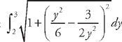 . Now we need to use some algebra to simplify the integrand:
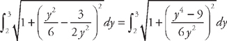 .
. .
. .
. .
. .
. .
. .
.
 (see
(see  from y = −
  to y =
 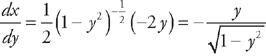 . Now we plug this into the formula for the length:
 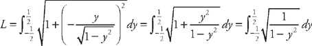 .
.
 (see
(see  . Now we plug this into the formula for the length:
 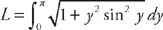 .
.
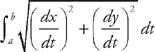 . Here, we have x = cos t and y = sin t from t =
  . First, we need to find the derivatives:
  and
and  . Now we plug this into the formula for the length:
  . Next, we use the trigonometric identity sin2 t + cos2 t = 1 to rewrite the integrand:
 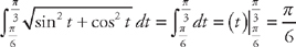 .
.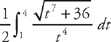
 . Here, we have x =
  and
and  from t = 1 to t = 4. First, we need to find the derivatives:
  and
and  . Now we plug this into the formula for the length:
  . With a little algebra, we get:
 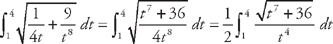 .
.
 . Here, we have x = 3t2 and y = 2t from t = 1 to t = 2. First, we need to find the derivatives:
  and
and  . Now we plug this into the formula for the length:
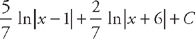
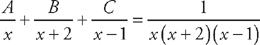
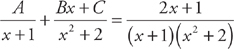
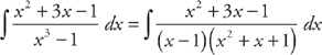
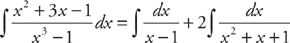
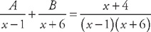 . First, we multiply through by (x – 1)(x + 6): A(x + 6) + B(x – 1) = x + 4.
 and
and  . This means that we can rewrite the integral as:
  . We can easily integrate these:
 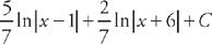 .
.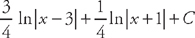
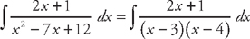
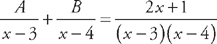
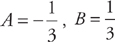
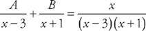 . First, we multiply through by (x – 3)(x + 1): A(x + 1) + B(x – 3) = x
 and
and  . This means that we can rewrite the integral as:
 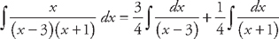 . We can easily integrate these:
  .
.
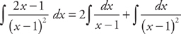
 .
. .
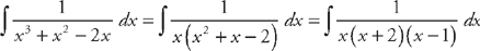
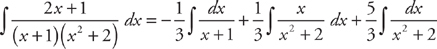
. , and
, and  . This means that we can rewrite the integral as:
 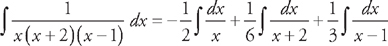 . We can easily integrate these:
 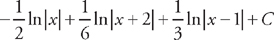 .
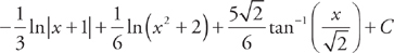
. .
. .
.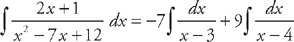 . We can easily integrate these: −7 ln |x − 3| + 9 ln |x − 4| + C.
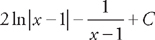
 .
. .
. .
.
 .
. , and
, and  .
. .
. . If you had trouble with these integrals, you should review the sections on logarithmic and trigonometric integrals.
 .
. , and
, and  .
. .
. . If you had trouble with these integrals, you should review the sections on logarithmic and trigonometric integrals.
 .
. .
. . The first integral is easy:
 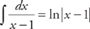 . The second takes a little work and will be a good test of your algebra. First, complete the square to rewrite the denominator:
 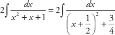 .
.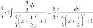 . This can be rewritten as:
  . Now we do u-substitution. If we let
  , then
  . Multiply du by
 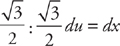 . Now we can substitute into the integrand:
 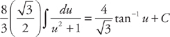 . Substituting back, we get:
 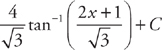 . Now we can put both integrals together:
  .
. . Now we evaluate the integral:
  . Finally, we take the limit:
 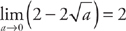 .
. and second, replacing the limit with a and taking the limit of the integral as a approaches 0,
 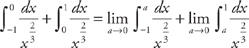 . Now we evaluate the integrals:
 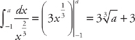 and
and 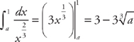 .
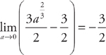
.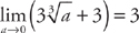 and
and 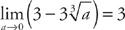 . Therefore, the integral is 3 + 3 = 6.
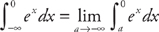 . Now we evaluate the integral:
  . Finally, we take the limit:
 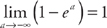 .
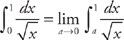
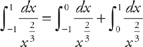
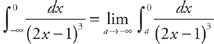
. is also undefined. We remedy this by replacing the upper limit with b and taking the limit of the integral as b approaches
  . And we overcome the two limits difficulty by splitting the integral into two parts at a value where we know that we can integrate and take each limit separately. A simple place to split the integral is at x = 0. We get:
  . Now we evaluate the integrals:
  and
and 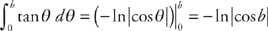 .
. and
and  . Neither limit exists, so the integral diverges. As a general rule, a trigonometric integral (but not an inverse trig one) is going to diverge if one of the limits of integration is infinite.
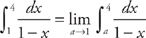 . Now we evaluate the integral:
  . Finally, we take the limit:
 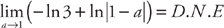 . Therefore, the integral diverges.
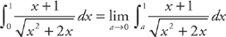 . Now we evaluate the integral. If we let u = x2 + 2x, then du = (2x + 2)dx. If we divide du by 2, we get
 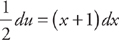 . Now we can substitute into the integrand. Let’s ignore the limits of integration until we substitute back. We get:
 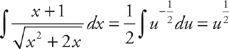 . Now we substitute back and evaluate at the limits of integration:
 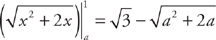 . Finally, we take the limit:
 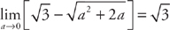 .
. . Now we evaluate the integral:
 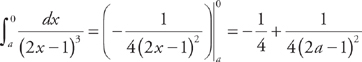 . Finally, we take the limit:
 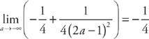 .
.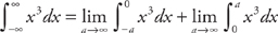 . Now we evaluate the integrals:
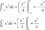
 and
and  . Therefore, the integral diverges. This is a tricky integral. Notice that if the limits of integration were finite and equal to each other, we would always get zero. It is easy to see this if we graph the function y = x3 and look at the areas on each side of the y-axis. They will always cancel each other because of symmetry.
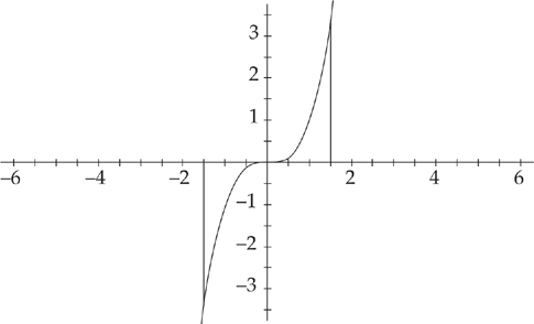
 and, second, replacing the limit with a and taking the limit of the integral as a approaches 2,
  . Now we evaluate the integrals:
  and
and  .
. and
and  .
. and second, replacing the limit with a and taking the limit of the integral as a approaches 0,
 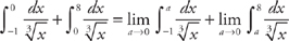 . Now we evaluate the integrals:
 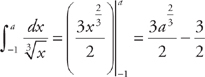 and
and 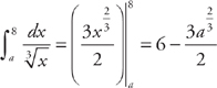 .
. and
and  . Therefore, the integral is
  .
.
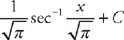
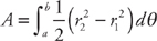
 (see
(see 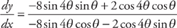 , which can be reduced to
 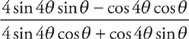 .
.
 (see
(see 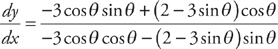 . Now we evaluate the slope at (r, θ) = (2, π):
  .
. (see
(see 
 . We can break this into three integrals:
  . We can easily evaluate the first two integrals:
  and
and  . The third integral requires us to use the trigonometric substitution
  (see
(see  . Therefore, the area is 18π.
 (see
(see 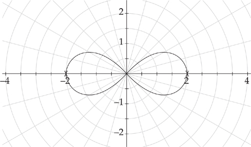
 to
to  . Plugging into the formula, we get:

 (see
(see 
 to
to  . Plugging into the formula, we get:
  . The first integral requires us to use the trigonometric substitution
  (see
(see  . The second integral is simply
  . Therefore, the area is
  .
.
 (see
(see 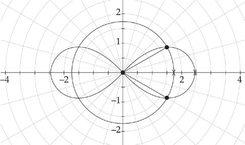
 to
to  . Plugging into the formula, we get:
  . Evaluating the integrals, we get:
  and
and  . Therefore, the area is
  .
.
 .
. .
.
 . Next, we integrate both sides:
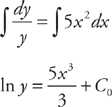
 . We can rewrite this as
  .
. .
.
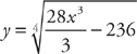
 . Next, we multiply both sides by y and by dx. We get:
  . Next, we integrate both sides:

 .
.


 .
. . Next, we integrate both sides:

 , which can be rewritten as y = 2x2.
 :
:
 , where k is a constant and y is the population at a time t. Here we are also told that y = 4,000 at t = 0 and y = 6,500 at t = 3. We solve this differential equation by separation of variables. We want to get all of the y variables on one side of the equals sign and all of the t variables on the other side. We can do this easily by dividing both sides by y and multiplying both sides by dt. We get:
  . Next, we integrate both sides:
 .
.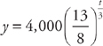 . Finally, we can solve for the population at time t = 10: y ≈ 4,000e.162(10) or
 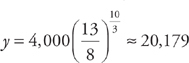 . (Notice how even with an “exact” solution, we still have to round the answer. And, if we are concerned with significant figures, the population can be written as 20,000.)
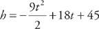
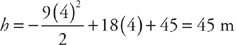
 . We are also told that v = 18 and h = 45 when t = 0. We solve this differential equation by separation of variables. We want to get all of the v variables on one side of the equals sign and all of the t variables on the other side. We can do this easily by multiplying both sides by dt: dv = –9 dt. Next, we integrate both sides:
 . We again separate the variables by multiplying both sides by dt: dh = (–9t + 18) dt. We integrate both sides:
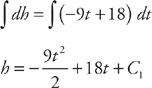
 , so C1 = 45
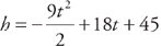 .
.
 where k is a constant and V is the volume of the sphere at time t. We are also told that V = 36π when t = 0 and V = 90π when t = 1. We solve this differential equation by separation of variables. We want to get all of the V variables on one side of the equals sign and all of the t variables on the other side. We can do this easily by dividing both sides by V and multiplying both sides by dt. We get:
  . Next, we integrate both sides:
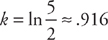
 . Finally, we can solve for the volume at time t = 3: V ≈ 36πe.916(3) ≈ 1766ft3 or
 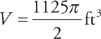 . (And, if we are concerned with significant figures, the volume can be written as 1800.)
 , where m is the mass at time t. We are also given that m = 10,000 when t = 0 and m = 5,000 when t = 5,750. We solve this differential equation by separation of variables. We want to get all of the m variables on one side of the equals sign and all of the t variables on the other side. We can do this easily by dividing both sides by m and multiplying both sides by dt. We get:
  . Next, we integrate both sides:
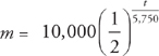 .
. . (And, if we are concerned with significant figures, the mass can be written as 8,900.)

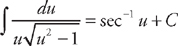
 , where a is the first term of the series and r is the common ratio (see
  . Plugging into the formula, we get:
  .
.
 , where a is the first term of the series and r is the common ratio (see
  . Plugging into the formula, we get:
  .
. and
and  . Plugging into the test, we get:
  . Therefore, the series converges.
 and
and  . Plugging into the test, we get:
 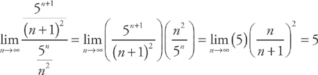 . Therefore, the series diverges.
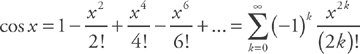


 .
. .
.

 . This simplifies to
 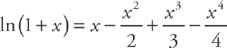 .
. .
.


 .
.


 , which simplifies to
 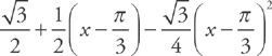 .
. ; the interval of convergence is
  .
.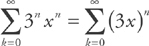 , so the common ratio is 3x. To find the interval of convergence, all
  . Thus the interval of convergence is
  . The radius of convergence is simply the distance from the center of the interval to either endpoint, or half the width of the interval. In this case, the radius of convergence is
 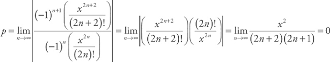 .
.


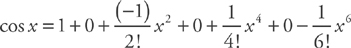
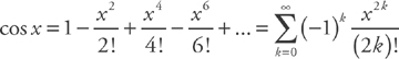
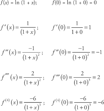
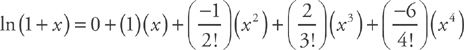
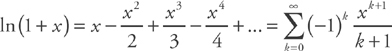
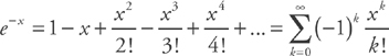
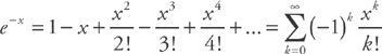
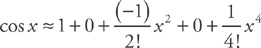 . This is the fourth degree Taylor polynomial. You should memorize the Taylor series that are highlighted on
  . To find the error bound, we can simply use the next term of the polynomial. Here, the next term is
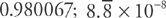
  . If we plug in x = 0.2, we get:
  .
.

 . This simplifies to
  .
. . To find the error bound, we can simply use the next term of the polynomial. Here, the next term is
  . If we plug in x = 0.3, we get: 0.002025.
 , so we need to see if
 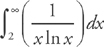 converges. First, we replace the upper limit with a
  . Next, if we let u = ln x, then
  . Substituting into the integrand, we get:
  . Substituting back, we get:
  . Finally, we take the limit:
  . Therefore, the series diverges by the Integral Test.
 , so we need to see if
 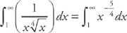 converges. First, we replace the upper limit with a and take the limit as a goes to infinity. We get:
 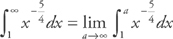 . Next, we integrate:
 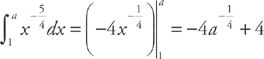 . Now, we take the limit:
 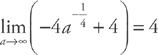 . Therefore, the series converges by the Integral Test.
 , which we can easily compare to the series
  . The series
  is essentially the harmonic series (it’s just missing the first two terms), which diverges. The series
 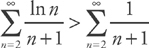 for all terms. Therefore, the series diverges by the Comparison Test.
 , which we can easily compare to the series
  . The series
  converges and the series
  for all terms. Therefore, the series converges by the Comparison Test.