MARK S. GOLDBERG AND GEOFFREY GARVER
1. INTRODUCTION
Ecological economics is concerned with incorporating into economic systems ecological and other constraints that neoclassical economics ignores. In this chapter, we discuss essential methodological considerations in making measurements to derive indicators that can be used to monitor the course of economic activity and the state of the environment so as to determine whether these constraints are being met.
For indicators to be useful, it is first important to define clearly why one wishes to measure them (in scientific inquiries, this would be referred to as the “objectives” of a research study or program) and then to ensure that the measurements are indeed measuring what they purport to measure (i.e., validity) and are consistent (i.e., reliability) (Koepsell and Weiss 2004). Contextual considerations affect the framing of these objectives and usually go to the heart of the questions being asked. Understanding what processes underlie indicators and what other factors or processes are associated with them (often referred to as “drivers”) are also important. For example, Ehrlich and Holdren (1972) suggested that the size of the human population, its affluence, and technology are essential drivers of environmental impacts, although many others will be important in specific circumstances. An example comes from air pollution and its effects on ecosystems (Lovett et al. 2009), where it is clear that combustion-related pollutants are due primarily to human activities. The interrelationships between different processes are often complex, requiring systems analysis or other techniques to help unravel the intricacies.
Challenges in measurement are compounded by the scale dependency of many ecological processes, varying from the local to the regional to the global. Many local processes scale up so as to have important aggregate effects at the global level. For example, local anthropogenic emissions of greenhouse gases, which vary geographically, in the aggregate are leading to changes in climate and other sequelae that are important at regional and global scales; in turn, those regional or global changes lead to impacts on life systems that vary across the globe (Intergovernmental Panel on Climate Change 2007). Measurement of the impact on ecosystems and species is also complicated by their ability to adapt. As well, there are important challenges in comparing metrics from ecosystems with different characteristics (commensurability). Heterogeneity of ecosystems (“a forest is not just a forest”) makes for diversity, but it may make difficult the interpretation of measurements and affect their generalizability to other systems, especially if the natural history of the ecosystem is not well understood or if there are no benchmarks for comparison. The heterogeneity of ecosystems and their interactions complicates the development of appropriate indicators that are important, valid, and reproducible.
A proposed methodological framework for measurements to support the development of indicators relevant to ecological economics is presented in the following sections. The framework has five elements: (1) contextual considerations, (2) considerations of scale and dimension, (3) considerations of scope, (4) considerations of commensurability, and (5) considerations of the interacting systems so that the paths leading to the indicator can be identified and targeted. We also discuss methodological aspects regarding what constitutes accurate measurements, as well as the myriad problems in interpreting indicators that comprise other primary ones (i.e., complex indicators).
2. CONSIDERATIONS OF CONTEXT
Contextual considerations concern the relationship of indicators to desired outcomes, as defined in terms of the objectives of ecological economics, including those derived from criteria based on considerations of ethics and justice. Questions regarding the application of indicators in a governance context are important; indicators must be developed not only in view of ethical and justice criteria, but also in view of practical issues regarding their application in governance and the means by which they are adopted and communicated.
One school of thought suggests that the state of ecosystems can be defined in terms of “ecosystem health” (Costanza 1992; Costanza and Mageau 1999; Jørgensen, Xu, and Costanza 2010; Rapport 1992; Suter 1993). Unfortunately, we show in chapter 6 that this concept, which has been developed in analogy with human health, is in fact vague and in practical terms of limited usefulness because of the difficulty of measuring all key domains. The essential consideration is that health, while an important concept, cannot be measured uniquely: it comprises multidimensional indicators that cannot be easily defined or measured. Indeed, Jorgensen indicated that “it is clear today that it is not possible to find one indicator or even a few indicators that can be used generally, or as some naively thought when ecosystem health assessment … was introduced” (Jørgensen 2010b). Thus, although it has been suggested that “ecosystem health [is] a comprehensive, multiscale, dynamic, hierarchical measure of system resilience, organization, and vigor” (Costanza and Mageau 1999), we argue that these constructs of resilience, organization, and vigor cannot be defined simply nor measured easily so as to portray the full range of function. Affirming these three specific attributes, or indeed any general combination, does not imply health.
To assess the contextual basis of the human–Earth relationship, biological and thermodynamic indicators (e.g., those in the eight categories in Jørgensen et al. [2010, 12–14]), more macroscale indicators like human appropriation of net primary production and ecosystem indicators,1 and social and economic indicators are certainly relevant but they do not define the entire space of function. In some sense, this should be obvious, although complex: the planet functions on many different spatial and temporal scales, and the processes that define these functions are myriad and highly interrelated, with many feedback loops built in. Moreover, the heterogeneity of ecosystems as well as “natural” secular changes makes it difficult to find norms by which to compare.
In light of these challenges, objectives derived from principles of ecological economics may provide context so as to allow the range of complexity with which indicators must contend to be reasonably managed. For example, the planetary boundaries concept (Rockström et al. 2009a, 2009b) discussed here and in the next chapter, provides a framework for deriving indicators based on the objective of maintaining the human economy so as to avoid changing the state of the planet to one that is not suitable for survival of many species, including humans.
3. CONSIDERATIONS OF SCOPE
Considerations of scope concern the range of parameters for which indicators are sought. For example, if the context is defined by an ethic of right relationship (Brown and Garver 2009), then it may be relevant to examine a broad range of human and social parameters in addition to environmental ones.
Issues of scope are thus related to issues of context. Presumably, the ethical and justice-based context for indicators will entail examining ecosystems and biogeophysical systems—not just in terms of biological, physical, and chemical parameters, but also parameters regarding the relationship of humans to each other, as well as their relationship to ecosystems and to the planet.
4. CONSIDERATIONS OF SCALE
Considerations of scale refer to the spatial and temporal scale of indicators. Scale is an essential element for consideration in developing indicators: some problems are global, such as climate change, yet both the changes that will occur and the local drivers of change will vary geographically and temporally. Other problems are local but may be present in several places in a region. For example, acid rain is a regional problem but its effects on lakes may be local; blue-green algae blooms are local to lakes and other waters but may be widespread in certain watersheds. Thus, it is essential to consider what indicators are appropriate and useful at different scales and how indicators at different scales interrelate. Indicators of the overall environmental condition of the planet may be useful in some contexts, but they may not necessarily be used to estimate the condition of a specific ecosystem or those in a region.
Scale also refers to time: some processes change slowly in time or have delayed feedbacks, whereas others may be more rapid (Rockström et al. 2009a, 2009b). Processes that usually work on geological time scales that are now showing changes over a few centuries, or even decades, are important to identify. For example, the increase in atmospheric carbon dioxide, which usually occurs over millennia, has been changing dramatically over a few decades. Evolution is clearly a slow process, but losses in biodiversity are occurring at much faster rates.
At the local ecosystem scale, the eight classes of biological and thermodynamic indicators in Jørgensen et al. (2010a) may be particularly relevant (see note 1) but nevertheless are incomplete. At this scale, one can attempt to characterize ecosystems by homeostasis, absence of disease, diversity or complexity, stability or resilience, vigor or scope for growth, balance between system components, and ecological integrity (“the interconnection between the components of the system”; Jørgensen 2010a). Specific indicators would need to be identified for each of these axes, and selection of indicators may vary with the context. Measures of function (“the overall activities of the system”) could be added, as well as other specific indicators that could be dependent on the type of ecosystem. It is not correct to think, however, that these indicators would comprise the universe of function.
At the global scale, relevant indicators of planetary function are those identified recently as useful for establishing “planetary boundaries for estimating a safe operating space for humanity with respect to the functioning of the Earth system” (Rockström et al. 2009a, 2009b). We discuss these in depth in the following chapter. The boundaries relate to climate change, ocean acidification, stratospheric ozone, global nutrient cycles, atmospheric aerosol loading, freshwater use, land use change, biodiversity loss, and chemical pollution. The global systems clearly interact in complex ways with systems at smaller scales, with complex feedback loops connecting them.
Another example comes from the indicator of human appropriation of net primary production, which can be relevant at local, regional, and global scales, and its correlation with species-energy curves, which relate the survival of species to the total production of available energy in a region. For example, by examining the effect of human appropriation of net primary production on the total energy available, Wright (1990) derived estimates of the percentage of species expected to be extinct or endangered; the estimates were found to be generally consistent with observations.
5. CONSIDERATIONS OF COMMENSURABILITY
Considerations of commensurability concern whether different measures can be reduced to a common one. The incommensurability of the value of thriving coral reefs with the value of fifty shares of ExxonMobil stock is at the heart of the debate over valuation of “ecosystem services” in terms of monetary value, which carries so much baggage of the standard neoclassical economic framework in which the value of money is defined. Indeed, the much-cited paper by Costanza et al. (1997) in which monetary values were assigned to ecological systems, while an attempt to gain ecological economics some weight in current policy debates, is clearly incompatible with the ethic and underlying rationale of ecological economics. Another example derives from the estimate that “wild” insects are worth $57 billion, and the conclusion that this value is “an amount that justifies greater investment in the conservation of these services” (Losey and Vaughan 2006). The absurdity of this specific assessment and conclusion—or for that matter any other monetized valuation of ecosystems or species—becomes clear when one considers the problems associated with the extinction of all or selected insects and the implicit assumption that insects, like all other goods, are replaceable at the cost of $57 billion or any other amount. The planet will be a dramatically different place should all of the bees become extinct (some research suggests that certain pesticides, neonicotinoids, may be the cause of bee deterioration; Henry et al. 2012; Whitehorn et al. 2012), and no amount of money could replace them and their essential functions. The challenge, then, is to avoid this problem of incommensurability in considering indicators of right relationship, and to develop ways to work toward desired objectives using decision-making techniques that involve consideration of indicators that are incommensurable with each other (Martinez-Alier et al. 2010).
Issues of commensurability raise questions of whether and how different ecosystems can be assessed in the aggregate, as well as how societal issues can be so assessed, and whether scorecard indicators that contain composites of incommensurable indicators provide useful information. Related to these issues are issues of controlling variables or indicators: Are some indicators more important than others in drawing conclusions about the functioning of an ecosystem or the planet? Can these indicators be used to develop sound policies that have a low probability of backfiring or simply failing? Also related to the question of commensurability is the nonlinear nature of the evolution of ecosystems, which complicates not only the reducibility of indicators to common metrics but also the use of at least some indicators prospectively. Lastly, this category of considerations includes issues of benchmarking and reference points, which are used extensively in assessing components of human health and in, for example, ecosystem restoration; however, they may be problematic in other areas.
Issues of incommensurability can be illustrated when asking whether composite indicators may be more useful than sets of indicators for the purposes of understanding functional status and for setting actions that may help improve function or mitigate environmental problems. Composite or aggregate indicators are those that express a complex aggregation of parameters, either in one unit of measure as does money or the ecological footprint, which makes use of derived functions to compute hectares of productive land; as a unitless index, such as the Sustainable Society Index; or as an indicator with uninterpretable dimensions (any quantities that have different units and are combined, either multiplicatively, additively, or in more complex ways will be difficult if not impossible to interpret). Examples of composite indicators include the following:
• Monetary value
• Gross domestic product, gross national product, and gross world product (expressed in monetary units, such as dollars)
• Various indicators used in material flow accounting (expressed in mass units [of biomass, minerals, etc.], per capita mass units, or percentages of the whole)
Many of these composite indicators take individual items (e.g., air quality, population growth, other composite indicators), multiply the value of each item by an assumption-laden weighting factor, and then add the products together. A generic indexing algorithm has been developed by Jollands, Lermit, and Patterson (2003). We have serious problems with this and any other methodology that combines disparate quantities measured in different units in essentially an arbitrary fashion. Our concerns are described below.
5.1. Limitations of Composite Indicators
While composite indicators are being used widely, most if not all suffer from serious issues of interpretation, including the following:
1. Mixing disparate quantities: The interpretation of a composite index in biological, physical, statistical, or other specific terms is often not possible because “apples and oranges” are mixed together. What does it mean to have a 7 for air quality added to a 5 for gender equality? That is to say, there is no clear construct that the index is purporting to measure. Moreover, without some benchmark or set of reference values, there is no way of interpreting composite indices except in a very general way, such as in concluding that a rising index is “good” and a falling index is “bad” (or vice versa); certainly, no policy decisions can be made using these indicators. Comparisons in terms of changes in time or comparisons between regions are always possible, but the meaning of the comparisons is obscure because of the difficulty in appreciating which components of the complex indicator are changing; this is usually impossible without detailed information about the individual components, and thus begs the question entirely as to the rationale for combining indices.
2. Combining information: Adding or multiplying components together, or using other more complicated mathematical functions (either attaching weights or not), is laden with assumptions that are not usually fully acknowledged, nor are their implications appreciated clearly. A key question is: what construct is actually being measured and how is it to be interpreted? In addition, uncertainties in the values of the index (e.g., statistical sampling variability, errors in measurement) may be overlooked or not identified. Other technical questions relate to the choice of the function to aggregate the different components and how to determine whether one mathematical function is superior to others.
3. Ambiguity in interpreting changes: Changes in a complex index, either temporally or spatially, cannot easily be attributed to the change of a specific component. For example, in the Sustainable Society Index, each of the twenty-two indicators is rescored on a scale from 0 to 10, then added together using assumption-laden weights to come up with a set of five summary values for each category (“personal development,” “health environment,” “well-balanced society,” “sustainable use of resources,” “sustainable world”). The scores for the categories are added together to obtain a final cumulative value. Such an index is impossible to interpret. For example, if one component increases to the same extent that another decreases, then there would be no change recorded. If there is change, it is not possible to determine where the change has occurred by simply inspecting the aggregate.
Here is a simple example: If two independent variables are summed or multiplied together, it is not possible to distinguish the meaning of any particular value of the sum or product. For example, how does one interpret an index that is computed as x1 + x2? If x1 = 4 and x2 = 5 or if x1 = 5 and x2 = 4, then the same result (9) is obtained, even though there may be large differences in what 9 means in the two cases.
4. Use in policy: Specific problems and solutions cannot be addressed using composite indicators, unless they are developed in such a way as to measure an important concept that has face or construct validity. For example, let us assume that “water quality” could be defined by adding together the concentration of individual pollutants (e.g., volatile organic substances, Escherichia coli, metals, turbidity). If the reason for measuring water quality is to prevent health problems in people, then interpretation of such an index would be obscure because some of the elements relate to long-term health effects (metals, volatiles), whereas others relate to short-term effects (E. coli, turbidity). There is no clear interpretation of adding concentrations of such disparate, and possibly correlated, quantities because it is impossible to benchmark the index—namely, determining what is a “safe” threshold.
On the other hand, various composite indices have been developed in public health policy, but these are used mostly for the purposes of communication with the general population to reduce their risk of contracting specific diseases. For example, the Canadian air quality index (Stieb et al. 2005; http://www.hc-sc.gc.ca/ewh-semt/air/out-ext/air_quality-eng.php; http://www.ec.gc.ca/cas-aqhi/default.asp?Lang=En) and the ultraviolet light index (http://www.epa.gov/sunwise/doc/what_is_uvindex.html) are used to inform people on a daily basis to reduce their burden of developing acute health effects from poor air quality and to reduce the long-term risk of developing skin cancer and cataracts from excessive ultraviolet light, respectively. These indices are not generally used to develop environmental policies. For example, the air quality index is derived from the actual concentrations of ozone, fine particles, and other pollutants; the associated health effects are used, with various political and economic constraints, to develop regulatory “acceptable” limits and actions. (The index has been used to estimate burden of disease [Stieb et al. 2005], but otherwise its main use is for the purposes of education and prevention.)
Some authors have suggested that composite indicators may be useful in a policy framework:
The costs of an aggregate indicator are that, if one is not careful and informed, one can be ignorant of where the numbers came from, how they were aggregated, the uncertainties, weights, and assumptions involved, etc. It’s not that one “loses” the more detailed information—usually it is possible to look at the details of how any aggregate indicator has been constructed—but rather that decision-makers are too busy to deal with these details. The beauty of the aggregate indicator is that it does that job for them. Even given this advantage of aggregate indicators, no single one can possibly answer all questions and multiple indicators will always be needed (Opschoor 2000), as will intelligent and informed use of the ones we have.
(Costanza 2000)
This assessment understates the problem of composite indicators, not least because it dismisses too easily the problem of busy decision makers misusing them. A composite indicator, unless benchmarked and understood in terms of the construct it is measuring, cannot be used appropriately in decision-making processes because it is unclear what is actually being measured. How can appropriate decisions be made on this basis? If, to have value in the decision-making process, composite indicators must be broken down into their individual components, then why not use the individual components to begin with? The fact that some politicians and bureaucrats cannot deal with sets of indicators does not justify the use (or, more likely, misuse) of composites.
Part of the problem that policymakers have in interpreting sets of indicators is that they lose sight of the reasons and clear objectives as to why they were collected. Thus, the policymaker is confronted with a morass of numbers that become uninterpretable and are out of context. Specifying in advance what are the problems and what needs to be measured maintains the context of the indicators.
6. CONSIDERATIONS OF THE MEASUREMENT PROCESS
The previous discussion on composite indicators leads naturally to a discussion of issues related to measurement and interpretation. As we indicated, one needs to be very clear about the reasons why something is being measured; in developing scientific projects, we refer to these as “operational objectives.” There is no reason to measure something just because it can be measured or is available, such as through administrative databases. An important adage is: “Not everything that counts can be counted, and not everything that can be counted counts” (sign hanging in Einstein’s office at Princeton University).
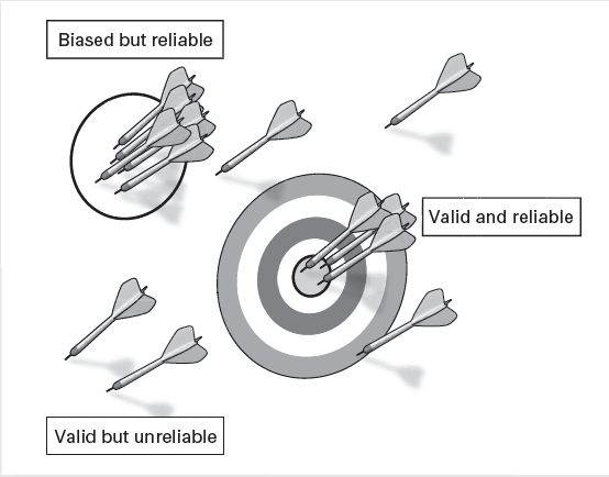
The objectives lead naturally to the specific constructs that one wishes to measure; this is often dictated by purpose but may be limited by knowledge and technology. An example of a well-defined construct is temperature: it defines the average kinetic energy of a system, is proportional to its heat content, and is bounded at the low end (0 Kelvin). It has face validity (see box 4.1 for a detailed description of the concepts of validity and reliability): that is, experts agree on what it measures. It also has content validity and construct validity: we understand from physical theory what is being measured. Depending on the actual instrument used, the variability in measurements of a system with exactly the same temperature can be very small (referred to as reliability, variability, or uncertainty). After repeated measurements by one or more unbiased instruments, the average will converge to the “true” temperature. Thus, the measurement of temperature is both valid and reliable (the two concepts together are often referred to as accuracy). Because temperature is valid and reliable, one can discern small trends through time, and it can be used in many instances as a sentinel indicator. Valid and reliable indicators are essential, not just in science but for the program of ecological economics.
Of course, the extent of the validity and reliability of a measurement will depend greatly on the inherent accuracy of the measurement instrument (figure 4.1). A judicious choice of instruments is needed for specific instances, taking into account how accurate the measures need to be. (In quantum experiments, one would never use a mercury bulb thermometer; to measure ambient temperatures, one would never use a device designed to measure at an accuracy of one in a billion.)
The case of global warming is instructive. To show that global warming is occurring, one needs to be certain that temporal trends cannot be explained by errors in measurement; that is, changes over time of the average measurements of ambient temperature across the planet are in fact larger than the errors of measurement (Brohan et al. 2006). Annual global mean temperature is assessed through monitors placed throughout the globe, so that the temperature recorded is representative of the temperature in a small area. The uncertainty in a “gridbox mean” caused by estimating the mean from a small number of point values is referred to as the sampling error. Because of costs and feasibility, not all parts of the globe are covered (i.e., coverage errors). There will also be uncertainties in the measurements at each station (i.e., station errors). Lastly, uncertainties in large-scale temperatures will arise because of changes in methods of measurement (i.e., bias error).
Mean global temperatures are built up as the average of the monitor-specific monthly or annual average. To appreciate whether the apparent secular, monotonic increase in temperature is increasing over and above error, an analysis of the global record can be undertaken. This analysis should account for the above-mentioned errors in measurement and coverage, such that the goal is to determine whether the increase in global mean temperature is greater than the total errors associated with the measurements. Figure 4.1 shows the results of an analysis combining the various errors, where the observed trends were greater than measurement error; therefore, the conclusion that the planet has been warming since 1850 was confirmed (Brohan et al. 2006). (A formal statistical analyses of these data leads to the same conclusions as perusing this figure.)
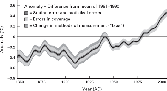
Figure 4.1. HadCRUT3 global temperature anomaly time-series (C) at smoothed annual resolutions. The solid black line is the best estimate value, the dark gray inner band gives the 95 percent uncertainty range caused by station, sampling, and measurement errors; the light gray band adds the 95 percent error range due to limited coverage; and the dark gray outer band adds the 95 percent error range due to bias errors. Source: Reproduced from Brohan et al. (2006).
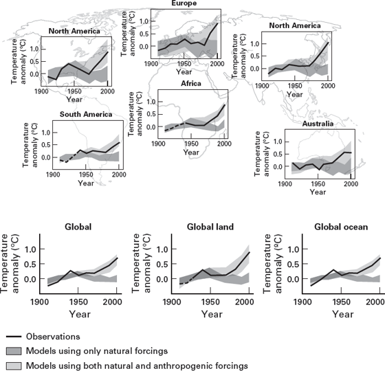
Figure 4.2. Comparison of observed continental- and global-scale changes in surface temperature with results simulated by climate models using either natural or both natural and anthropogenic forcings. Decadal averages of observations are shown for the period 1906–2005 (black line) plotted against the centre of the decade and relative to the corresponding average for the 1901–1950. Lines are dashed where spatial coverage is less than 50 percent. Dark gray bands show the 5 percent to 95 percent range for nineteen simulations from five climate models using only the natural forcings due to solar activity and volcanoes. Light gray bands show the 5 percent to 95 percent range for fifty-eight simulations from fourteen climate models using both natural and anthropogenic forcings. Source: Reproduced from Intergovernmental Panel on Climate Change (2007).
Of course, this particular example says nothing about regional changes in temperature. In fact, we know that areas of the north are warming much faster than near the equator (figure 4.2) (Intergovernmental Panel on Climate Change 2007). Thus, global mean temperature is a restricted indicator of planetary change that obscures strong spatial heterogeneity. As a physical indicator, global mean temperature is nevertheless important because it reflects the extra energy added to the atmosphere from increased climate forcing, which is due mostly to increased anthropogenically-induced greenhouse gas emissions.
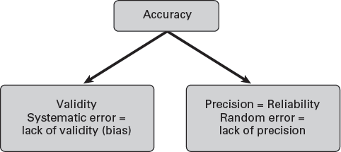
Figure 4.3. The paradigm of accuracy.
This example of global warming shows clearly the importance of analyzing measurements by time to determine trends; it also shows the intimate link between measurement and statistics. The paleoclimatic record suggests that the current concentration of greenhouse gases is far greater than what existed over the last 600,000 years, and there is indeed concern that continued increases in greenhouse gas emissions will lead to global warming that could melt the polar icecaps. Such a nonlinear, irreversible change (a “tipping point”) could lead to a major catastrophe, by causing crops to fail and flooding of much of the earth’s land masses. One could then think that, in fact, there is a “normative” standard that can be identified by perusing the paleoclimatic record; some suggest that it is close to 350 ppm of carbon dioxide (Rockström et al. 2009a, 2009b), and we have gone well past that (approximately 400 ppm as of December 2014; http://co2now.org). With a trend of annual increases of almost 2 ppm, the world is heading for concentrations on the order of 450–500 ppm before long.
7. MODELS AND PREDICTION
Scientific measurements are often used to develop models that can make predictions where there are no data, such as projecting into the future or to other situations. All models have a range of validity, and no statistical models or physical models are perfectly accurate. The question is whether the models are useful. Understanding their limitations is obviously critical if they are to be used in in ecological economics and in policy. All models need to be validated.
The difference between models and measurements should be made clear: measurements are a real-time representation of some construct (e.g., concentrations of a pollutant in a watershed), whereas models can be developed to predict concentrations where measurements were not made (e.g., a spatial prediction model) or, with additional information, to project into time what these concentrations may be. To interpret these models correctly, all of the assumptions built into these models need to be made clear. The value of these models comes only when further measurements are made that show that the model is correct (or not). Sometimes, the models provide generally correct projections, but their estimates may not be 100 percent accurate (this is the usual case). In such an instance, it is likely that the model incorporates the correct science but may be lacking details, such that its quantitative accuracy is not as good as one would hope.
It is important to distinguish between the different types of models that can be developed. Although it is impossible to discuss all of the types of models that are used, we can present a few examples that may provide the reader with some notion of how these are used. Returning to our example of global temperature, one can develop statistical models to project into time what the expected global temperature will be in a certain year in the future (e.g., 2100). Such a model would make use of all of the available historical data (inputs) and would attempt to find the “best-fitting” function to describe these data (output). One of the simplest functions is a straight line, but in fact this does not represent the best line because the rate of change of temperature increased dramatically around 1970–1980 (the so-called hockey-stick graph). However, once one has found the correct function (if one assumes that the trend remains the same through time), then one can project the value of the function through time to arrive at a prediction for 2100 (this projection would also incorporate the associated statistical variability). Clearly, this is a crude model because of the assumption that the conditions that led to changes in temperature will remain the same in the future.
Climate modelers have developed far more sophisticated models, called global circulation models. These models make use of the known physics, including various feedback mechanisms, to integrate possible changes to concentrations of greenhouse gases through different sets of scenarios of anthropogenic emissions. Not every model will arrive at the same prediction because each model has different assumptions built in; also, because of computational complexity, some models may try to make the physics a bit simpler than in others. The models are being continuously updated to include new physics and new information and are tested on past data.
Comparing predictions to observations tests the extent of the usefulness of models. The general circulation models have been used to back-project temperatures in the twentieth century; that is, by using estimates of emissions during the twentieth century (input), the models were run to see if they predicted the set of already observed global temperatures (comparison of predicted to observed values). Indeed, the average across the models was shown to follow observed temperatures. This validation gives confidence that the models projecting into the future will provide plausible predictions; it provides some range of variability, but does not guarantee that the future will correspond with these predictions (Intergovernmental Panel on Climate Change, 2007).
Not all indicators in ecological economics need be used for prediction. However, they will clearly be needed for assessing secular and spatial trends, and perhaps for regulating economic activity. Therefore, knowing the attributes of the indicators, in terms of validity and reliability, is essential.
8. CONSIDERATIONS OF COMPLEX INTERACTING SYSTEMS
As part of defining any indicator, one must be cautious in its interpretation because it may derive from complex processes within and between interacting systems. There are always limitations to measurement and also to predictability; complex systems are subject to unpredictable behavior and thus unpredictable outcomes. This is not just a limitation of measurement, it is an inherent behavior of complex systems. This view contrasts with one stating that “there is an objective truth out there; if we only had enough time and money, we could get enough measurements and build good-enough models that we could model the future with precision.” Complex systems theory includes the idea of “irreducible uncertainty.” Thus, much care must be given to defining indicators, the models that they are based on, and their interpretation. The precautionary principle, discussed in the next chapter, provides one way in setting policy to deal with uncertainty, especially as it relates to decisions of policy.
Many of the indicators that we consider in the next chapter are global in nature. Nevertheless, the underlying processes act on local and regional scales, and there are many complex feedback loops. We will discuss the concept of setting constraints on the human economy in the form of boundary values that have been proposed to allow the planet to function safely for humanity. To be able to make these boundaries into normative values that should not be crossed, it is essential to be able to have a top-down approach that is able to set limits at small geographic scales.
Two examples should suffice. Again, using climate change, we know that anthropomorphic emissions of carbon occur locally and that international agreements are based on national quotas. Much work has been done to show the link between various sectors and emissions, as well as between atmospheric concentrations of greenhouse gases (globally more or less uniform) and emissions levels. Thus, global targets for the atmospheric concentration of greenhouse gases can be met by meeting national targets for emissions.
An example of the phosphorus cycle also may be useful. This is a key indicator (see chapter 5), and phosphorus is used as an essential nutrient in agriculture. Overuse and runoff has led to massive build-ups in various water systems, including in northwest European countries (Ulén et al. 2007), the Gulf of Mexico from runoff from the Mississippi and other river systems that flow to the Gulf of Mexico, and also in lakes where there is runoff from farms. This has led to eutrophication, apoxia (oxygen deficiency), and growth of algae blooms, such as the toxic blue-green algae (Ulén et al. 2007). Phosphorus is a useful indicator in ecological economics because its build-up in local waterways can be compared to levels that avoid those problems using other methods of farming, and those limits can be scaled up to establish a global boundary for phosphorus.
For ecological economics to be successful in its goal of recognizing the embeddedness of human activities in the planet, setting global constraints on phosphorous is essential to reducing the damage on ecosystems. Setting and enforcing constraints can only be done effectively by assessing regional patterns (for the Gulf of Mexico, this entails thousands of square kilometers), which requires accurate measurements. It also requires a full understanding of the pathways by which phosphorus enters ecosystems, which requires complex models, either based on empirical data (statistical models) or mechanistic models. Validation of the models is a sine qua non for their use, but once in place they can be used to set and enforce regional and local constraints. Having set constraints is, of course, insufficient; one needs alternative modes of agriculture so that reductions can be implemented, as well as methods to buffer runoff. Some efforts to reduce population are needed, as this is a key driver. Educational programs and possibly incentives to implement these new agricultural policies would also be required.
9. CONCLUSIONS
We have discussed the essential properties that indicators need to have for their appropriate use in ecological economics and in making policy decisions. In particular, we showed that clear objectives are required so that one understands exactly what should be measured and why. As well, we discussed various issues associated with the measurement process, but we also discussed the elements that can be used to help define what indicators should be measured by considering context, scale and dimension, scope, and commensurability. As part of this process, one needs to consider interrelationships between variables and attempt to recognize the complexity that may affect the interpretation of the measurements. We indicated that sound scientific principles must be followed so that the measurement process is accurate (valid and reliable). The extent of the inherent variability of the measurements will be dictated by the circumstances, but certainly appreciating the errors will facilitate understanding. We have cautioned strongly about using complex indicators because they will rarely measure a meaningful construct; thus, the interpretation of their values will typically be obscure. These principles apply to both the key processes and their drivers.
BOX 4.1. ISSUES RELATED TO MEASUREMENT
Use of any indicator is dictated solely by the objectives. Without clear objectives, interpretation is difficult and development of specific measures logically impossible. A prima facie criterion for any indicator is that it is valid and reliable (Koepsell and Weiss 2004). This means generally that the indicator measures what it purports to measure and does with a known level of uncertainty. Thus, not only must one determine what and how to measure a quantity, but one must also assess level of error associated with the measurements.
There are many aspects to validity; we present here a few of the main concepts. Face validity of a measure refers to whether it is obvious that it will measure what it is supposed to measure, such as measuring physical quantities. Experts can agree that a certain index measures what it purports to measure. This type of validity often applies to physical and certain biological measures, but often, even in physics, measures are developed that have a certain interpretation but are derived from other measures. Entropy, an essential concept in thermodynamics, is a derived quantity, but theory has developed to make it an essential quantity.
One can say that a measure such as entropy corresponds to the concept of construct validity. It refers to the degree to which inferences can be made from an index with respect to the theoretical construct it is supposed to measure. In another example, back pain has many etiologies and manifests itself differently in people. Is there a way of measuring the extent to which back pain affects one’s daily life? One index that has been in use for many years is the Roland-Morris Low Back Pain and Disability Questionnaire (Roland and Morris 1983a, 1983b). It comprises twenty-four questions, as follows:
THE ROLAND–MORRIS LOW BACK PAIN AND DISABILITY QUESTIONNAIRE
I stay at home most of the time because of my back.
I change position frequently to try to get my back comfortable.
I walk more slowly than usual because of my back.
Because of my back, I am not doing any jobs that I usually do around the house.
Because of my back, I use a handrail to get upstairs.
Because of my back, I lie down to rest more often.
Because of my back, I have to hold on to something to get out of an easy chair.
Because of my back, I try to get other people to do things for me.
I get dressed more slowly than usual because of my back.
I only stand up for short periods of time because of my back.
Because of my back, I try not to bend or kneel down.
I find it difficult to get out of a chair because of my back.
My back is painful almost all of the time.
I find it difficult to turn over in bed because of my back.
My appetite is not very good because of my back.
I have trouble putting on my sock (or stockings) because of the pain in my back.
I can only walk short distances because of my back pain.
I sleep less well because of my back.
Because of my back pain, I get dressed with the help of someone else.
I sit down for most of the day because of my back.
I avoid heavy jobs around the house because of my back.
Because of back pain, I am more irritable and bad tempered with people than usual.
Because of my back, I go upstairs more slowly than usual.
I stay in bed most of the time because of my back.
Each item refers to the construct of functioning in the “presence of back pain.” The degree of back pain could also be measured by asking questions that rate the levels of pain. The Roland-Morris questionnaire is often used giving a response of “yes” the value of 1; a “no” response is given the value of zero. Adding-up the scores across the twenty-four questions, giving equal weight to each question, leads to an index that is bounded on the low end by zero (no problems) to twenty-four (problems with all functional assessments). This index is thus a simple count (no units) of problems that an individual is having at the time of the assessment. Of course, one can always assess the individual indicators by themselves. This composite index is of course not useful for decisions about diagnoses or treatment, but it is very important for the individuals suffering from back pain and is also very useful in assessing treatments and differences between groups of individuals. Indeed, a comparison of the mean of this complex indicator between two populations would lead to a statistical inference as to whether one population has more functional problems with back pain than another. Such an assessment would not state specifically what the functional problems are; only assessing each item would provide that information. Assessing a population in time would allow the answer to the question regarding longitudinal physical functioning because of back pain. This index has construct validity, but it is not the only index that can be used to measure back pain or functioning. When to use this or any other index is driven by the questions that one wants to answer.
There are a number of formal definitions of construct validity. For example, the US Environmental Protection Agency (EPA) defines it as “the extent to which a measurement method accurately represents a construct and produces an observation distinct from that produced by a measure of another construct” (www.epa.gov/evaluate/glossary/c-esd.htm). The previous examples meet this definition.
The Roland-Morris questionnaire contains a number of related items that are combined into a composite index. Each item corresponds to a slightly different aspect of functioning with back pain, but the main concept is to measure functioning with back pain. This is referred to as content validity; the EPA defines it as “the ability of the items in a measuring instrument or test to adequately measure or represent the content of the property that the investigator wishes to measure” (www.epa.gov/evaluate/glossary/c-esd.htm).
There are other aspects related to validity (e.g., criterion validity; sis.nlm.nih.gov/enviro/iupacglossary/glossaryc.html), but it is not necessary to discuss these any further here.
Of considerable interest, however, is the issue of reliability (uncertainty or variability), which is related to measurement error but also to statistical variability. There is an inherent error associated with any measurement process, and one of the key ideas of measurement theory is to develop instruments that have a minimum amount of measurement error. In measuring temperature, we discussed in the main text the concepts of “station error” and “bias error,” which described inherent errors from the measurement process across the temperature monitors across the globe and through time. Indeed, if these errors were too large, then any real increase in global temperature would not be identifiable. Reliability can thus be defined as the inherent amount of variability in the measurement process.
Other forms of reliability exist. If one has different individuals assessing a trait, then each individual’s assessment of a specific case may vary in time because of subtle changes in the process. This is referred to as an interrater agreement. When there are many raters, even if the same criteria are being used, there will also be variability between raters, and this is referred to as inter-rater variability.
In statistics, the concept of reliability is often referred to as statistical variability or statistical error. Statistical error refers to sampling variability: the results of a study on a specific population will not be the same if a different population was selected randomly. If one had enough resources, one could repeat a study many times and the average of the results across the studies would reflect the best estimate; the amount of variability in these estimates is the sampling error. There is a clear link between this concept and measurement error; if the errors in measurement are not known, then they will be subsumed within statistical variability. However, if the measurement error is known, then it can be partitioned from the total variability. Essentially, statistical variability refers to variation that cannot be readily explained; indeed, one of the goals of statistics is to explain this variability. (The identification of drivers, say in the IPAT formulation [Ehrlich & Holdren 1972], could be viewed in this light if data are available.)
Often the concepts of validity and reliability are viewed together, and this is often referred to as accuracy (see figure 4.3). On the other hand, the term “accuracy” is often used to represent validity.
Figure 4.4. The difference between reliability and validity. Source: Nancy E. Mayo, McGill University.
1. Jørgensen et al. (2010, 12–14) identified eight levels of indicators for the assessment of “ecosystem health,” based on the following: (1) the presence or absence of specific indicator species; (2) the ratio between classes of organisms; (3) the presence, absence, or concentrations of specific chemical compounds, such as phosphorous, in regard to trophic level or toxic chemicals in regard to toxicity; (4) the concentration of trophic levels, such as the concentration of phytoplankton as an indicator of eutrophication of lakes; (5) process rates, such as the rate of primary production in relation to eutrophication or the rate of forest growth in relation to forest health; (6) composite indicators, including E.P. Odum’s attributes and various indices, such as total biomass or the ratio of production to biomass; (7) holistic indicators, such as biodiversity, resilience, buffer capacity, resistance, and turnover rate of nitrogen; and (8) “superholistic” thermodynamic indicators, such as exergy (the energy in the ecosystem available to do work), energy, and entropy.
REFERENCES
Brohan, P., J. J. Kennedy, I. Harris, S. F. B. Tett, and P. D. Jones. 2006. “Uncertainty Estimates in Regional and Global Observed Temperature Changes: A New Data Set from 1850.” Journal of Geophysical Research: Atmospheres 111 (D12): D12106. doi:10.1029/2005JD006548.
Brown, Peter G., and Geoffrey Garver. 2009. Right Relationship: Building a Whole Earth Economy. San Francisco: Berrett-Koehler Publishers.
Costanza, Robert. 1992. “Toward an Operational Definition of Ecosystem Health.” In Ecosystem Health: New Goals for Environmental Management, edited by Robert Costanza, Bryan G. Norton, and Benjamin D. Haskell, 239–256. Washington, DC: Island Press.
Costanza, Robert. 2000. “The Dynamics of the Ecological Footprint Concept.” Ecological Economics 32: 341–345.
Costanza, Robert, Ralph d’Arge, Rudolf de Groot, Stephen Farber, Monica Grasso, Bruce Hannon, Karin Limburg, Shahid Naeem, Robert V. O’Neill, Jose Paruelo, Robert G. Raskin, Paul Sutton, and Marjan van den Belt. 1997. “The Value of the World’s Ecosystem Services and Natural Capital.” Nature 387 (6630): 253–260. doi: 10.1038/387253a0.
Costanza, Robert, and Michael Mageau. 1999. “What Is a Healthy Ecosystem?” Aquatic Ecology 33 (1): 105–115. doi: 10.1023/A:1009930313242.
Ehrlich, Paul R., and John P. Holdren. 1972. “Critique on ‘the Closing Circle’ (by Barry Commoner).” Bulletin of the Atomic Scientists 28 (5): 16, 18–27.
Henry, Mickaël, Maxime Béguin, Fabrice Requier, Orianne Rollin, Jean-François Odoux, Pierrick Aupinel, Jean Aptel, Sylvie Tchamitchian, and Axel Decourtye. 2012. “A Common Pesticide Decreases Foraging Success and Survival in Honey Bees.” Science 336 (6079): 348–350. doi: 10.1126/science.1215039.
Intergovernmental Panel on Climate Change. 2007. Fourth Assessment Report, Climate Change 2007: Synthesis Report. Edited by The Core Writing Team, Rajendra K. Pachauri and Andy Reisinger. Geneva: Intergovernmental Panel on Climate Change.
Jollands, Nigel, Jonathan Lermit, and Murray Patterson. 2003. “The Usefulness of Aggregate Indicators in Policy Making and Evaluation: A Discussion with Application to Eco-Efficiency Indicators in New Zealand.” Australian National University Digital Collections, Open Access Research. http://hdl.handle.net/1885/41033.
Jørgensen, Sven Erik. 2010a. “Eco-Exergy as Ecological Indicator.” In Handbook of Ecological Indicators for Assessment of Ecosystem Health, edited by Sven Erik Jørgensen, Fu-Liu Xu, and Robert Costanza, 77–87. Boca Raton, FL: CRC Press.
Jørgensen, Sven Erik. 2010b. “Introduction.” In Handbook of Ecological Indicators for Assessment of Ecosystem Health, edited by Sven Erik Jørgensen, Fu-Liu Xu, and Robert Costanza, 3–7. Boca Raton, FL: CRC Press.
Jørgensen, Sven E., Fu-Liu Xu, João C. Marques, and Fuensanta Salas. 2010. “Application of Indicators for the Assessment of Ecosystem Health.” In Handbook of Ecological Indicators for Assessment of Ecosystem Health, edited by Sven Erik Jørgensen, Fu-Liu Xu, and Robert Costanza, 9–75. Boca Raton, FL: CRC Press.
Jørgensen, Sven Erik, Fu-Liu Xu, and Robert Costanza, eds. 2010. Handbook of Ecological Indicators for Assessment of Ecosystem Health. 2nd ed. Boca Raton, FL: CRC Press.
Koepsell, Thomas D., and Noel S. Weiss. 2004. “Measurement Error.” In Epidemiologic Methods: Studying the Occurrence of Illness, 215–246. Oxford: Oxford University Press.
Losey, John E., and Mace Vaughan. 2006. “The Economic Value of Ecological Services Provided by Insects.” BioScience 56 (4): 311–323. doi: 10.1641/0006–3568(2006)56[311:TEVOES]2.0.CO;2.
Lovett, Gary M., Timothy H. Tear, David C. Evers, Stuart E. G. Findlay, B. Jack Cosby, Judy K. Dunscomb, Charles T. Driscoll, and Kathleen C. Weathers. 2009. “Effects of Air Pollution on Ecosystems and Biological Diversity in the Eastern United States.” Annals of the New York Academy of Sciences 1162 (1): 99–135. doi: 10.1111/j.1749–6632.2009.04153.x.
Martinez-Alier, Joan, Giorgos Kallis, Sandra Veuthey, Mariana Walter, and Leah Temper. 2010. “Social Metabolism, Ecological Distribution Conflicts, and Valuation Languages.” Ecological Economics 70 (2): 153–158. doi: 10.1016/j.ecolecon.2010.09.024.
Opschoor, Hans. 2000. “The Ecological Footprint: Measuring Rod or Metaphor?” Ecological Economics 32 (3): 363–365. doi: 10.1016/S0921–8009(99)00155-X.
Rapport, David J. 1992. “Evaluating Ecosystem Health.” Journal of Aquatic Ecosystem Health 1 (1): 15–24. doi: 10.1007/BF00044405.
Rockström, Johan, Will Steffen, Kevin Noone, Asa Persson, F. Stuart Chapin, III, Eric F. Lambin, Timothy M. Lenton, Marten Scheffer, Carl Folke, Hans Joachim Schellnhuber, Bjorn Nykvist, Cynthia A. de Wit, Terry Hughes, Sander van der Leeuw, Henning Rodhe, Sverker Sorlin, Peter K. Snyder, Robert Costanza, Uno Svedin, Malin Falkenmark, Louise Karlberg, Robert W. Corell, Victoria J. Fabry, James Hansen, Brian Walker, Diana Liverman, Katherine Richardson, Paul Crutzen, and Jonathan A. Foley. 2009a. “Planetary Boundaries: Exploring the Safe Operating Space for Humanity.” Ecology and Society 14 (2): 32. http://www.ecologyandsociety.org/vol14/iss2/art32/.
Rockström, Johan, Will Steffen, Kevin Noone, Asa Persson, F. Stuart Chapin, III, Eric F. Lambin, Timothy M. Lenton, Marten Scheffer, Carl Folke, Hans Joachim Schellnhuber, Bjorn Nykvist, Cynthia A. de Wit, Terry Hughes, Sander van der Leeuw, Henning Rodhe, Sverker Sorlin, Peter K. Snyder, Robert Costanza, Uno Svedin, Malin Falkenmark, Louise Karlberg, Robert W. Corell, Victoria J. Fabry, James Hansen, Brian Walker, Diana Liverman, Katherine Richardson, Paul Crutzen, and Jonathan A. Foley. 2009b. “A Safe Operating Space for Humanity.” Nature 461: 472–475. doi: 10.1038/461472a.
Roland, Martin, and Richard Morris. 1983a. “A Study of the Natural History of Back Pain. Part I: Development of a Reliable and Sensitive Measure of Disability in Low-Back Pain.” Spine 8 (2): 141–144.
Roland, Martin, and Richard Morris. 1983b. “A Study of the Natural History of Low-Back Pain. Part II: Development of Guidelines for Trials of Treatment in Primary Care.” Spine 8 (2): 145–150.
Stieb, David M., Marc Smith Doiron, Philip Blagden, and Richard T. Burnett. 2005. “Estimating the Public Health Burden Attributable to Air Pollution: An Illustration Using the Development of an Alternative Air Quality Index.” Journal of Toxicology and Environmental Health, Part A 68 (13–14): 1275–1288. doi: 10.1080/15287390590936120.
Suter, Glenn W., II. 1993. “A Critique of Ecosystem Health Concepts and Indexes.” Environmental Toxicology and Chemistry 12: 1533–1539. doi: 10.1002/etc.5620120903.
Ulén, B., M. Bechmann, J. Fölster, H. P. Jarvie, and H. Tunney. 2007. “Agriculture as a Phosphorus Source for Eutrophication in the North-West European Countries, Norway, Sweden, United Kingdom and Ireland: A Review.” Soil Use and Management 23: 5–15. doi: 10.1111/j.1475–2743.2007.00115.x.
Whitehorn, Penelope R., Stephanie O’Connor, Felix L. Wackers, and Dave Goulson. 2012. “Neonicotinoid Pesticide Reduces Bumble Bee Colony Growth and Queen Production.” Science 336 (6079): 351–352. doi: 10.1126/science.1215025.
Wright, David Hamilton. 1990. “Human Impacts on Energy Flow through Natural Ecosystems, and Implications for Species Endangerment.” Ambio 19 (4): 189–194. doi: 10.2307/4313691.