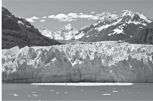
Fig. 18-0: Glaciers in Alaska’s Glacier Bay. Such glaciers are remnants in North America of the vast ice sheets that covered the northern half of the continent during ice ages of the past million years. (© Bart Everett with permission under license from Shutterstock image ID 5134369)
On geological timescales Earth’s climate preserved liquid water at the surface, thanks to the tectonic thermostat discussed in Chapter 9. Within this stability, Earth’s climate also undergoes significant change on intermediate timescales of 104–105 years that can greatly influence living conditions. These changes occur because climate is sensitive to details of planetary orbital variations. Earth spins with a tilted axis and equatorial bulge, causing it to precess like a top about every 20,000 years. Because of the gravitational tug of the major planets, Earth’s orbital tilt and orbital shape change cyclically on the timescales of 40,000 and 100,000 years. Scientists now believe that the changes in the seasonal and latitudinal distribution of the sunlight reaching Earth generated by these orbital cycles (called Milankovitch cycles) paced waxing and waning of Earth’s ice caps. Extensive records of these changes over the past 800,000 years have been obtained from ice cores in Greenland and Antarctica. While the forcing functions of orbital variations would lead to sinusoidal change, the ice age cycles are not simple sinusoids. Instead, ice ages end abruptly and are entered gradually, suggesting complex feedbacks must influence them. The ice age cycles also correlate closely with atmospheric CO2 and CH4, probably with a slight lag compared to ice volume. While the link with Milankovitch forcing is evident, many details of the diverse manifestations of ice ages remain to be fully understood. The ocean with its large CO2 reservoir and complex behavior must play an important role, as may induced volcanism from melting ice sheets that adds a pulse of CO2 to the atmosphere during deglaciation. From 5–1 Ma, orbital forcing caused ice ages to vary on a 40,000-year (40 Ka) cycle rather than 100 Ka cycle. Prior to 5 Ma there were no northern hemisphere ice ages. Prior to 30 Ma there was no Antarctic ice sheet. In ice-free periods, orbital forcing must also have operated to induce intermediate scale climate change, though the specifics of these ancient influences on climate are currently not well described.
The high temporal resolution of the ice-core records also reveals striking short-term climate change over 101–103 years. Such changes are likely modulated by jumps in climate from one of its quasi-stable states of operation to another. The causes of such short-term change also remain to be fully understood, and they may be triggered by reorganizations of the ocean’s thermohaline and atmospheric circulation. Intermediate and short-term climate change have major consequences for the habitability of continents. The exit from the last glacial advance 11,000 years ago and the following benign climate of the current interglacial have permitted the migration of human beings throughout the continents, vast population growth, and the rise of human civilization.
As we look at Earth today the ice sheets of Greenland and Antarctica appear to us as permanent features. The fossil record shows us that this was not always the case—alligators and lush forests once occurred in polar regions, showing that large changes in Earth’s global climate have occurred during the Phanerozoic. And in the Precambrian, the proposed “snowball Earth” episodes show that climate variations can be even more extreme. These changes all occur over millions of years, extremely long even with respect to the rise of Homo sapiens some 150,000 years ago. On shorter timescales, is climate locked into relative stability? Might there be climate changes on timescales that would be pertinent to human history and human future? Our recognition of vast change in the positions of continents, the composition of the atmosphere, and the evolution of life were all broadened and informed by observations from Earth’s geological record. As we will see in this chapter, large changes in Earth’s climate that would be of great significance to modern life have also characterized the geological record. While over millions of years Earth’s climate is remarkably stable in the preservation of liquid water at the surface, on short timescales the climate is fickle in ways that have major consequences for life. These changes can occur on short enough timescales to be pertinent to the history and future of human civilization.
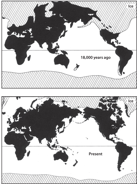
Evidence suggesting a recent ice age came to light through studies of Louis Agassiz in the nineteenth century. By careful examination of Alpine glaciers, he noted that striations on rocks, U-shaped valleys, and transport of large blocks of rock were characteristic of glacial behavior. Similar features occurred in central Europe and also at great distances from the modern extent of glaciers in the Alps. He noted that transport by glaciers could explain huge exotic boulders lying in open plains in northern Europe, and that distinctive heaps of debris (known as moraines) could be explained if they were bulldozed into place by the advancing ice. Furthermore, glaciers could be observed making distinctive landforms such as U-shaped valleys that contrasted with the V-shaped valleys of river erosion, and the mountains in Switzerland, Scotland, and Scandinavia had long and vast valleys that appeared to have been excised by glaciers. Estimates of the areal extent of these vast continental ice sheets could be constructed by mapping the extent of glacial striations on bedrock and by the moraines, showing that vast ice sheets once covered much of Europe and North America (Fig. 18-1). Estimates of the volume of these ice sheets can be made from the extent to which sea level was lowered. A record of sea-level lowering provided by fossil man-grove roots preserved along the margins of Indonesia indicate that, at its maximum, sea level was lowered about 120 m. In other words, in order to create these great ice sheets, a layer of seawater about 120 m thick across the entire ocean had to be transformed into ice. The last glaciation also had to have been recent, because the loose glacial sediments were very well preserved, and rivers running in the U-shaped glacial valleys had created only small incisions in the valley floors.
Fig. 18-1: Maps contrasting the extent of ice cover during the peak of the last period of glaciation, 20,000 years ago, with that which exists at present: Part of this ice is continental and part floats in the sea. (Map courtesy of George Kakla)
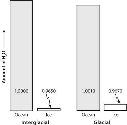
In the second half of the twentieth century, much greater precision on the timing and magnitude of glaciations was obtained from sediments deposited on the seafloor. The tool that revealed the glacial record with great precision was variations in oxygen isotope compositions preserved in the shells of tiny-shelled organisms, called benthic foraminifera, which inhabit the seafloor. As we learned previously, stable isotopes can be fractionated by low temperature processes. The process of evaporation of water near the equator and its transport and precipitation as ice near the poles causes the ice in ice caps to have an 18O/16O ratio 3.5% (35 per mil) lower than that for seawater. Like the difference in carbon isotopes between organic and inorganic carbon discussed in Chapter 16, the offset between polar ice and liquid ocean is quite constant. At the same time, the total 18O/16O ratio of all of Earth’s water has a defined average value that does not change. As the ice sheet grows, and more and more water with low 18O/16O is removed from seawater, the seawater 18O/16O increases as the mean value of total H2O is preserved (Fig. 18-2). Therefore, just as we were able to use carbon isotopes to determine the proportions of organic and inorganic carbon in Chapter 16 (see Fig. 16-2), the oxygen isotopes can be used to determine the proportions of ice and liquid water. A caveat must be mentioned here, which is that the 18O/16O of the shells is also influenced by the water temperature. Fortunately cold temperatures that would also be associated with glacial conditions also lead to higher 18O/16O in the shells, so the stable isotope record gives a clear signal of glacial vs. interglacial conditions. Work by Dan Schrag and colleagues suggests that about half the change can be associated with temperature and about half with ice volume.
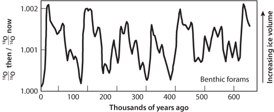
Shown in fig. 18-3 is the 18O/16O record obtained from shells picked from various depths in a sediment core from the deep tropical ocean. As amazing as it may seem, these tiny organisms provide us with a record of changes in continental ice volume. Low values of 18O/16O show low ice volume and high values high ice volume. By using radioactive dating, a firm absolute timescale has been obtained for this record. What the record shows is that there have been multiple ice ages extending back about 700,000 years. The record is “sawtooth” in shape, with a long slow slide (increasing 18O/16O in the figure) into the deepest ice age. The cooling ends with an abrupt termination to low ice volume and a brief and warm interglacial period, such as what we are now experiencing. While there is much fine structure to the record, the dominant period of change is about 100,000 years, which can be observed by noting the positions of the interglacials in the figure (times with lowest 18O/16O).
Fig. 18-2: Comparison of the amounts of H2O in the ocean (as water) and in the continental glaciers (as ice) during times of full interglaciation (like today) and during times of full glaciation (such as 20,000 years ago): The heights of the bars indicate the amount of water in each reservoir. The numbers associated with the bars are the 18O/16O ratio for the H2O divided by the 18O/16O ratio in today’s ocean. Since the ice is about 3.5 percent depleted in 18O compared to seawater, the expansion of ice sheets causes the ocean to become slightly enriched in 18O. See Fig. 16-2 for an analogous relationship for the carbon isotopes and the fraction of organic and inorganic carbon.
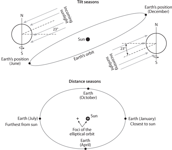
The realization by geologists that Earth’s climate has undergone dramatic cycles brought with it a curiosity as to what caused these shifts. From the very first, the prime candidate has been the cyclic changes in Earth’s orbit about the sun. Although when averaged over long periods of time Earth’s path around the sun remains unchanged, its orbit does show some repetitive deviations from this mean. The importance of these orbital changes lies in the fact that they alter the contrast between the seasons. Changes in the seasonal distribution of the sunlight received at any given location on Earth’s surface are driven by two characteristics of its orbit. The first is associated with the tilt of Earth’s spin axis with respect to the plane of its orbit about the sun (see Fig. 18-4). Earth’s spin axis does not stand straight up. Rather, it leans away from the vertical by an angle of about 23°. Consequently, on June 21 the Northern Hemisphere faces the sun. Six months later, on December 21, the Southern Hemisphere faces the sun. If Earth stood straight up, its equator would always face the sun and there would be no tilt-induced seasons. The larger the tilt, the greater the seasonal range in the amount of radiation received at any point on the globe.
Fig. 18-3: The 18O/16O record in benthic foraminifera for a sediment core from the deep Pacific Ocean. The 18O enrichment in the glacial-age shells is partly the result of growth of the ice sheets and partly the result of colder deep ocean temperatures. This record reveals that the 100,00-year cycle, which has dominated climate for the past 750,000 years, is asymmetrical. Long intervals of bumpy cooling are terminated by abrupt warmings.
Also shown in Figure 18-4, a second source of seasonality exists. It relates to the fact that Earth’s orbit is slightly out of round. In geometric terms, the orbit is an ellipse. As you remember, circles can be drawn by tying a string to a piece of chalk. The end of the string is held at the center (focus) of the circle and the circle is drawn by swinging the chalk around. An ellipse has two foci. To draw an ellipse, both ends of the string are pinned down, one at each focus. The chalk is not attached; rather it is nested freely in the vee made by the stretched string. The ellipse is drawn by swinging this vee around. The farther apart the foci, the more eccentric the ellipse—i.e., the more it deviates from circularity. No planet has a perfectly circular orbit, all are elliptical. The laws of gravity require that one of the two foci of the planet’s orbit corresponds in location to the sun. The consequence of the elliptical shape of Earth’s orbit is that the Earth-sun distance changes over the course of the year. When closer to the sun, Earth receives more radiation; when farther away, it receives less.
Fig. 18-4: Seasonality and its cyclic changes. This diagram shows the factors that influence the seasonal contrast in the radiation received at any point on the globe. The primary cause of seasons is the tilt of Earth’s axis with respect to its orbit about the sun. Upper panel: As shown here, this tilt leads to higher illumination of the Northern Hemisphere during June and to higher illumination of the Southern Hemisphere during December. Our calendar is set so that June 21 and December 21 correspond to the days on which maximum radiation falls on the Northern Hemisphere and on the Southern Hemisphere, respectively. A second contribution to seasonality stems from the fact that the Earth’s orbit is elliptical. Because of this, the Earth-sun distance changes during the course of the year. Lower panel: As shown here, currently Earth is closest to the sun early in January and farthest from the sun early in July. Thus Earth as a whole receives less sunlight during July than during January.
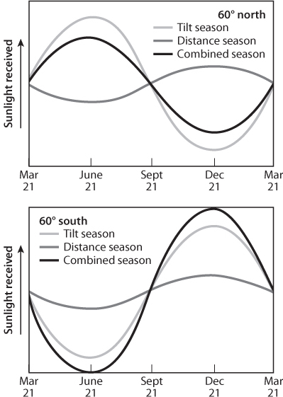
Fig. 18-5: Comparison of the seasonal cycles of solar illumination at 60°N and 60°S: In the Southern Hemisphere the tilt and distance seasons currently reinforce one another. In the Northern Hemisphere they currently oppose one another.
Shown in Figure 18-5 is the relationship between the two seasonal cycles. Currently in the Northern Hemisphere they oppose one another. The reason is that the Northern Hemisphere leans toward the sun as it traverses that portion of its orbit farthest from the sun. By contrast, the Southern Hemisphere leans toward the sun as it traverses that portion of its orbit closest to the sun. Hence, the two sources of seasonal contrast (tilt and distance) currently oppose one another in the Northern Hemisphere and reinforce one another in the Southern Hemisphere.
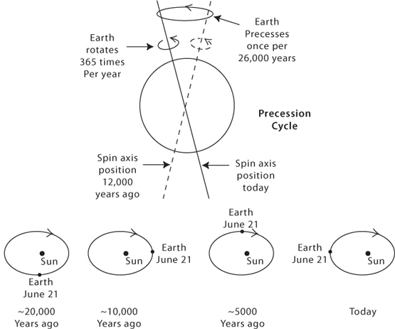
Our interest in all this arises because the situation changes with time. The reason for this is that Earth precesses as does a spinning top. Both precess for the same reason: their spin axes tilt. The leaning top precesses to keep from falling. The leaning Earth precesses to keep its equatorial bulge from becoming aligned with its orbit, i.e., pointing directly at the sun. Just as a top spins much more rapidly than it precesses, so also does Earth. It takes Earth 8,760,000 days (26,000 years) to complete one precessional cycle. At the same time the elliptical orbit rotates slowly, and the combination of the two leads to approximately 21,000 year period in the variations of solar insolation from precession.
Fig. 18-6: Like a top, Earth’s spin axis precesses: It takes about 26,000 years for one complete precession cycle. Precessions change the point on Earth’s orbit where maximum Northern Hemisphere illumination occurs. Today it occurs at the “long” end of the ellipse, reducing full summer illumination in the Northern Hemisphere. The ellipse itself is also rotating and the net effect of the two leads to a 21,000 year cycle. One-half precession cycle ago (i.e., ∼10,500 years ago) it occurred at the “short” end of the ellipse, increasing full summer illumination a bit. The precession of Earth’s axis relates to the sun’s pull on the equatorial bulge produced by Earth’s rotation. Just as Earth’s gravity seeks to tip over a spinning top, the sun’s gravity seeks to remove the tilt of Earth’s axis. As does a top, Earth compensates for this pull by precessing.
The importance of precession to seasonality is that it causes a progressive change in Earth’s location in its orbit on June 21 (Fig. 18-6). Eleven thousand years ago the Northern Hemisphere faced the sun as Earth traversed that part of its orbit nearest to the sun. Hence, at that time the tilt and distance seasons reinforced one another in the Northern Hemisphere, and thus the precession of Earth causes the contrast between the seasons to change in a cyclic manner.
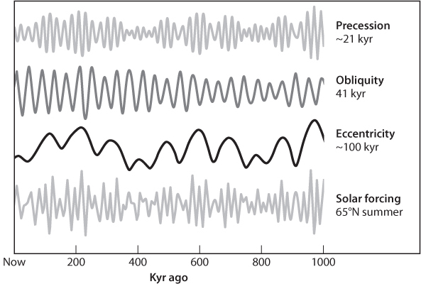
Fig. 18-7: The precession and obliquity of Earth’s spin axis and the eccentricity of its orbit as a function of time, and their effect on summer insolation at 65°N. Axial tilt varies by two degrees. Eccentricity varies from 0.01 to 0.05. These records are reconstructed from calculations based on the law of gravitation and the present-day orbits and masses of the planets. (modified from en.wikipedia.org/wiki/File:Milankovitch_Variations.png)
In addition to its precession, Earth’s orbit is subject to two other cyclic changes. Both have to do with the gravitational pull of our sister planets, particularly Jupiter. These tugs cause the eccentricity of Earth’s orbit to change with time. At times it has been even more eccentric than it is today and at times it has been less. The more eccentric the orbit, the stronger the distance seasonality. The interplanetary tugs also lead to changes in Earth’s tilt. The greater the tilt, the greater the seasonal contrast; the smaller the tilt, the smaller the seasonal contrast. The time histories of both eccentricity and the tilt of the orbit can be calculated very precisely from knowledge of the masses of the planets and their orbits. The results of these reconstructions are shown in Figure 18-7. As can be seen, the tilt cycle is quite regular, the highs being spaced at 40,000-year intervals. While the eccentricity changes have a more complex pattern, the highs are spaced at intervals of about 100,000 years.
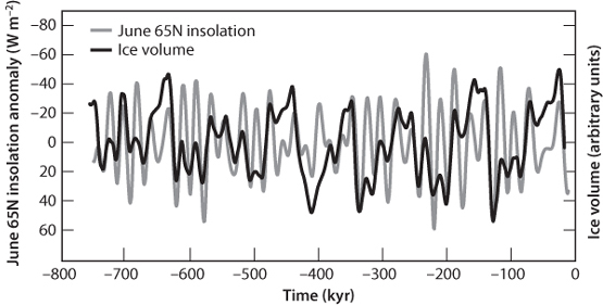
Fig. 18-8: Comparison of summer insolation with the record of ice volume, with the ice volume shifted with a lag of 6,000 years to maximize the fit between peaks and valleys in each record. The insolation axis is reversed so that low values of insolation give high values on the y-axis. While there is a general correspondence, the fit is by no means perfect. (Figure modified from G. Roe, Geophys. Res. Lett. 33 (2010), L24703)
Earth’s precession, the changes in its tilt, and the changes in the eccentricity of its orbit combine to yield a complex history in seasonal contrast. This record is different for different latitudes. The influence of changes in tilt is most prominent at high latitudes, while the influence of distance changes is the same at all latitudes. In Figure 18-8 is shown the average daily radiation received during the month of July at 65°N (the latitude around which the ice caps of glacial time were centered) compared with changes in ice volume. At this latitude the amount of radiation received varies by about 100 watts/m2.
The benthic 18O record (i.e., ice volume) is compared with the summer sunshine record for 65°N in Figure 18-8 with a time offset of 6,000 years between the two records. While the two curves are quite different, they show some intriguing similarities. Low ice volume corresponds with the periods of high anomalies of solar insolation (e.g., near 600 Ka and 200 Ka), and the second-order “wiggles” in the record match closely in the time that they occur (but not the amplitude). John Imbrie quantified these correspondences and showed that the characteristic wavelengths of the climate record corresponded with the precession and tilt frequencies. This result was accepted as evidence for an orbital cause to climate variations.
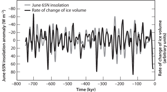
Fig. 18-9: The same insolation record as Fig. 18-8 now compared to changes in ice volume rather than absolute ice volume. High values of solar insolation (low values of the light gray line in the figure) correspond to ice sheets losing volume more rapidly. Note the close correspondence of the ~20 Ka cycles. No lag is required in the ice volume record to match the insolation record. (Figure modified from G. Roe (2010))
More recent work adopts a slightly different approach with an even more compelling result. Because the continents are largely in the Northern Hemisphere, Northern Hemisphere insolation has the major effect on ice sheets. But ice sheets are big, and therefore one bright summer will not suddenly cause them to disappear. Instead, peaks in solar insolation should cause the most rapid change in the ice sheet volume. So, rather than the absolute size of ice sheets, it should be the temporal change in size of the ice sheet that matches variations in solar insolation. Gerard Roe of Washington University carried out such an analysis, which is shown in Figure 18-9, with no time lag between records. The correspondence is obvious—more summer sunlight corresponds with maximum changes in ice volume. These results clearly pose the Milankovitch hypothesis of orbital variations on climate: changes in solar insolation caused by orbital variations have a major influence on the temporal change in ice volume. In this form the Milankovitch theory ranks a 9 on our theory scale—orbital variations induce climate change.
While these correspondences between the summer-sunshine record and the ice-volume record have convinced most geophysicists that changes in Earth’s orbital characteristics have somehow paced glacial cycles, the detailed nature of the connection remains incompletely understood, and many puzzles remain.
One puzzle is the rapid exit from glacial maxima to interglacial conditions. The orbital variations are all sinusoidal in form, so that increases and decreases in solar energy are symmetrical. The 18O/16O record, however, is not sinusoidal. Instead it shows a long slow decline to a glacial maximum, followed by an abrupt termination to an interglacial warm period, creating a “sawtooth” ice volume record rather than a sinusoidal one. This result can also be seen in the rate of change in ice volume. Inspection of Figure 18-9 shows that generally the black line of change in ice volume has lower amplitude than the gray insolation line, except at the times of the 100 Ka deglaciations, when particularly large changes in ice volume occur.
Another puzzle is the change in composition of the atmosphere that corresponds with changes in ice volume. Tiny gas bubbles trapped in the ice in Greenland and Antarctica have permitted a detailed record of change in atmospheric composition over the last 750,000 years. CO2 and CH4 vary coherently with ice volume, with high CO2 and CH4 corresponding to the warm interglacials and low values corresponding to glacials. Careful investigation of the records suggests that the atmospheric changes lag slightly in time the ice volume changes, so that ice volume decreases first, followed by atmospheric change. Why should formation and destruction of ice sheets, which are made up only of water, be associated with variations in CO2?
These results suggest there are positive feedbacks associated with the ends of ice ages. Lowering of ice volume causes rise in greenhouse gases CO2 and CH4, which would then lead to further warming and loss of ice volume. A great deal of energy has gone into trying to fathom the causes of the sawtooth temperature and CO2 records. One likely possibility is the ocean, because it contains fifty times more CO2 than the atmosphere does. If interglacial changes somehow led to decarbonation of the ocean, then that could cause a rise in atmospheric CO2, which would lead to further warming and cause a rapid termination. The exact mechanism of such an oceanic response, however, remains unclear.
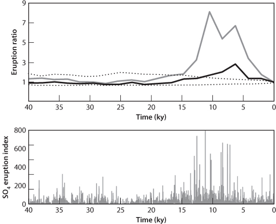
Another possibility is that the glacial terminations are influenced by a feedback between ice sheets and volcanism. As we learned previously, magma production is sensitive to pressure changes. When ice sheets melt, they rapidly remove mass from the continents to the oceans, depressurizing the continental mantle and pressurizing the oceanic mantle. On Iceland, this led to a massive burst of magmatism that followed the removal of an ice sheet 2 km thick that covered the island during the last glaciation. Working with Icelandic colleague Dan McKenzie and coworkers has shown that this volcanic outpouring can be explained by increased melting due to the pressure changes in the mantle. The link with CO2 would come from volcanic degassing. Because most of the CO2 flux to the atmosphere comes from convergent margins, increased volcanism there could have a significant effect on the CO2 budget. Data on volcanic eruptions shows that global continental volcanism increased by three to five times during the last deglaciation (Fig. 18-10). The extra volcanism would contribute more CO2 to the atmosphere, leading to greater warming, more ice sheet melting, and more CO2 addition. This process appears capable of accounting for about half the positive feedback that would be needed to explain the sawtooth records. It also has the appeal that it provides a single mechanism to explain rapid glacial terminations and the lag in the rise of atmospheric CO2.
A final puzzle of Earth’s response to orbital variations is the change in the period of ice ages over the last 2 million years. Figure 18-11 shows a 1.8 Ma record of glaciations based on sediment cores. Prior to 0.8 Ma, the dominant period of ice age cycles was 40,000 years, corresponding with changes in tilt. Then suddenly the dominant period changed to 100,000 years. This change is mysterious because the 100,000-year cycle corresponds to eccentricity, and eccentricity variations have very small effects on solar insolation. Revisiting Figure 18-8, for example, the 100,000-year cycle is not particularly evident in the changes in solar insolation but completely dominates the ice volume record. How can such small signals be amplified to produce such a large glacial signal, and why did the period change 1 million years ago?
On a final note, the last 2 million years have provided a clear record of orbital variations because they have been expressed as ice ages (e.g., Fig. 18-11). In other periods of Earth’s history, ice sheets were not present (Fig. 18-12). Why? It seems likely that positioning of the continents at high latitudes may be a crucial influence, but the overall understanding of why some periods of Earth’s history have ice ages and some do not remains unclear. How orbital variations may have influenced climate in ice-free conditions is also an open question. Sediment records from Eocene and Cretaceous rocks have been found to show regular variations in composition that can be “tuned” to Milankovitch frequencies (it is very difficult to get very precise ages in these time intervals). It appears that even in the absence of ice, global climate change may have been important, but the mechanisms and specifics remain to be fully elucidated. While orbital variations are clearly important for climate changes on the 104–106 year timescale, much remains to be understood in this rapidly evolving field.
Fig. 18-10: Plot of global changes in volcano eruption frequency during the exit from the last glaciation. The last glacial maximum at 17 Ka is marked by low volcanic output. From 15 Ka to 5 Ka volcanoes erupt about four times more frequently than the glacial background, pumping CO2 into the atmosphere and contributing to temperature rise and further ice melting. Volcanoes erupt also large amounts of SO2, and the lower panel shows the volcanic pulse is recorded as sulfate in the Greenland ice core. (Figure modified from Huybers and Langmuir (2009) Earth Planet. Sci. Lett. 286 (2009):3-4 479)
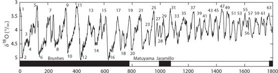
Fig. 18-11: A 1.8 Ma record of ice volume showing the change from a 40 Ka cycle prior to 1 million years ago to the 100 Ka cycle evident in more recent data. The 40 Ka cycle persists all the way back to the beginning of recent glaciations 5 million years ago. These changes remain to be fully understood. (Figure from Lisiecki and Raymo, Paleooceanography 20 (2005), PA1003)
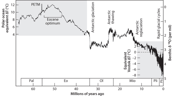
Fig. 18-12: A broader time perspective on climate change. The benthic oxygen isotope record records ice volume. Prior to 30 Ma there was no Antarctic ice sheet and no ice ages. Northern Hemisphere glaciations began about at about 5 Ma. The increased importance of orbital forcing to ice volume beginning at that time is apparent from the δ18O record. (Figure from Wikipedia Commons, based on data from Zachos et al. Science 27 April 2001, 686–93)
An even shorter timescale of climate change is revealed in the detailed climate records preserved in ice cores from Greenland and Antarctica. Long borings extending from the surface to bedrock provide an extremely detailed record covering the last 110,000 years (i.e., back to the middle of the last interglacial period) in Greenland and back to 750,000 years in Antarctica. The 18O/16O ratio in the ice provides a proxy for local air temperature, the calcium content of the ice a proxy for dust infall, and the methane content of air bubbles trapped in the ice a proxy for tropical wetness. In addition to the stately cycles of tens of thousands of years in duration, steep-sided millennial oscillations occur with surprising frequency. Even more surprisingly, these proxies reveal that during glacial time a series of large and abrupt changes in climate occurred (see Fig. 18-13). Intervals of extreme cold, high dust, and low methane alternated with intervals of lesser cold, lower dustiness, and higher atmospheric methane content. The transitions between these climate states were abrupt, taking place in as little as a couple of decades.
Why does this record look so different from the stable isotope record of most seafloor sediments? Two reasons can be given. First of all, in ice cores annual layers are preserved, while the deep-sea sediment record has been smoothed by the stirring action of bottom-dwelling worms, which churn these muds to depths of up to 10 cm. As the accumulation rates for the majority of these sedimentary records are in the range 2–5 cm per thousand years (as opposed to 10–20 cm per year in Greenland ice), signals associated with the millennial-duration events have been obliterated. Second, the large glacial-age ice sheets in Canada, Scandinavia, and Antarctica were too sluggish to respond significantly to millennial-duration climate changes. Hence these events are not imprinted on the benthic 18O record, which is recording large changes in ice volume.
Unlike the 100,000-year climate cycle and its ~21,000- and 40,000-year modulations that are close to synchronous across the globe, the millennial record in Antarctica ice is antiphased with respect to that in Greenland ice. Across the Northern Hemisphere, however, these changes are in lockstep. Greenland’s ice core reveals not only changes in local air temperature but also changes in the atmosphere’s dustiness and its methane content. Measurements of the isotopic composition of strontium and neodymium serve as a fingerprint of the source of the dust and show that Greenland’s dust originated in the great Asian deserts, suggesting that the frequency of intense storminess over Asia changed in harmony with Greenland’s air temperature. During glacial time, the wetlands of Canada, Scandinavia, and Siberia, which currently serve as the source for about half of the atmosphere’s methane, were either frozen or buried beneath mile-thick ice sheets. Because of this, during glacial time the global production of methane was smaller and confined largely to the tropics. If so, then the abrupt shifts in methane content recorded in Greenland ice suggest that tropical rainfall was lower during Greenland’s millennia of intense cold than during the intervening milder intervals.
Evidence for the impacts of these millennial-duration events appears in other records. For example, deep-sea cores from the northern Atlantic reveal distinct episodes during which large numbers of icebergs were released into the sea from the ice sheets surrounding this basin. Upon melting, the rock fragments trapped in these bergs fell to the seafloor, creating ice-rafted debris. Radiocarbon dating demonstrates that these layers formed at the times of Greenland’s intense millennial cold spells. Consistent with this evidence are paleotemperatures obtained for a high-accumulation-rate, deep-sea sediment core from deep ocean floor close to Bermuda. The measurements suggest that during glacial time the surface ocean temperatures jumped back and forth by 4° to 5°C in synchrony with the millennial-duration events in Greenland. The 18O record for a stalagmite from China suggests that the strength of monsoonal rains varied in harmony with Greenland’s temperature. The monsoons were weaker during the episodes of intense cold.
Strong evidence also comes from the most recent of these short-term fluctuations. The last glacial maximum occurred at 17,000 years, followed by a characteristic abrupt warming event. But then, from 13,000 to 11,000 years ago Earth plunged into a temporary reentry to glacial conditions called the Younger Dryas. This event is strikingly evident in the Greenland ice-core record (see Fig. 18-13). As might be expected, high mountain regions are very sensitive to cooling, leading to large down-mountain expansions of their ice caps. Radiometric dating of debris pushed out as the glaciers advanced allow the most recent epochs of mountain cold to be correlated with Greenland’s most recent cold phase. So far it has been demonstrated that glaciers in the Swiss Alps, in the tropical Andes, and New Zealand’s Alps underwent major readvances when Greenland ice last revealed a millennial-scale cold period.
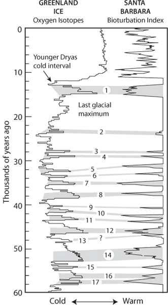
Fig. 18-13: Comparison between the air temperature record in Greenland and the O2 content record for the bottom waters in the Santa Barbara basin: The latter is based on the extent of burrowing of the sediment by worms. At times of high O2, the annual layering in the sediment is completely obliterated by the action of these organisms in a process called “bioturbation.” At times of low O2, the worms can’t survive and the annual layering is perfectly preserved.
To this evidence from mountain glaciers can be added an impressive record from the sediment in a small basin located between Santa Barbara, California, and Santa Rosa Island (Fig. 18-13). As sediments accumulate in this basin at the rate of 1 m per 1,000 years, a record of millennial changes is beautifully preserved. At present the O2 content of its bottom water is so low, and the rain of organic matter so high, that the water that fills the sediment pores is devoid of O2. The anoxic conditions make the environment uninhabitable for worms, which under oxic conditions continually mix the uppermost sediment in a process called bioturbation. Under anoxic conditions, no stirring occurs and the sediments have annual laminations reflecting the seasonal variations in the mix of biological and soil debris reaching the bottom.
Interested to see how far this layered record extended back in time, Jim Kennett, a marine geologist at the University of California at Santa Barbara, initiated a program to core this basin. Annually layered sediment continued uninterrupted back to the beginning of the present interglacial (i.e., to about 11,000 years ago), but below that lies a long series of alternating zones of bioturbated sediment and annually layered sediment. Kennett quickly realized that the intervals of well-mixed sediment must represent times when the O2 content of deep water in the Santa Barbara basin was higher than now. When he compared his record to that from the Greenland ice core, he found an incredible match (Fig. 18-13). At the times of extreme cold in the ice core, a layer of well-stirred sediment accumulated in the Santa Barbara basin. Kennett concluded that this meant that the invasion of freshly oxygenated surface waters into the intermediate depths of the northern Pacific Ocean had greatly strengthened at these times. More recently, German scientists obtained a nearly identical record in the rapidly accumulating sediment in the Arabian Sea off Pakistan.
Taken together, this paleoclimatic evidence suggests that the impacts of the millennial-duration climate episodes so obvious in the Greenland ice core were widespread. There is, however, a tantalizing exception. The record in ice cores from Antarctica reveals that during the 10,000-year-long transition from full glacial conditions to full interglacial conditions, the millennial-duration modulations of climate were antiphased with respect to those recorded in Greenland. When the Northern Hemisphere experienced the pre-Younger Dryas warm spell, the warming in Antarctica stalled. When conditions in the Northern Hemisphere were plunged into the Younger Dryas cold, Antarctica resumed its warming. Thus, while the orbital-related cycles were globally synchronous, the millennial-duration changes appear to have been antiphased. Furthermore, at least in the case of the Younger Dryas, the boundary between the two realms curiously enough appears to lie to the south of New Zealand rather than at the equator.
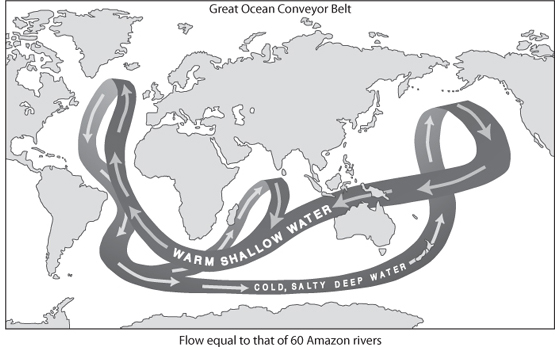
The millennial-duration shifts in climate constitute a challenging mystery. What is it about Earth’s climate system that allows it to undergo large and abrupt climate changes? Why are these changes antiphased between Antarctica and the rest of the planet? Why has no such change taken place during the last 10,000 years? What triggers these jumps? While convincing answers have yet to emerge, some clues suggest that the instigator lies in the ocean. Model simulations suggest that the ocean’s so-called thermohaline circulation is capable of undergoing reorganizations. This large-scale circulation is driven by the descent to the abyss of cold and salty water from two places on the planet, the northern Atlantic in the vicinity of Iceland and the Southern Ocean along the perimeter of the Antarctic continent. Currently, the northern source floods the deep Atlantic with water that sweeps southward, passing around the tip of Africa, where it joins waters rapidly circulating around the Antarctic continent. Deep waters formed around the perimeter of Antarctica also sink into this circumpolar current, producing a mix that currently consists of roughly equal amounts of the two source waters. Portions of this mixture peel off and move northward into the deep Indian and Pacific oceans (Fig. 18-14).
These currents are important to Earth’s climate because they redistribute heat. This redistribution is especially important for the land masses surrounding the northern Atlantic. Replacing the water sinking to the bottom of the northern Atlantic are warm upper ocean waters carried northward toward Iceland in the upper limb of the conveyor. As this upper limb traverses the low latitudes, it is heated by the sun. When it reaches high northern latitudes, this stored heat is released to the overlying air. During winter months, this heat takes the sting out of the cold Arctic air masses that move eastward across the Atlantic. This bonus of heat helps to sustain northern Europe’s mild winters.
The magnitude of the conveyor transport by the conveyor is staggering. It equals that of a hundred Amazon Rivers and matches rainfall across the entire globe. The northward moving limb carries water with an average temperature of 12°C into the region around Iceland. The water sinking into the abyss averages only 2°C. Hence, for each cubic centimeter of water carried northward by the conveyor’s upper limb, 10 calories of heat are released to the atmosphere. This adds up to a staggering total, equaling about one-quarter of the solar heat supplied to the atmosphere over that portion of the Atlantic Ocean lying to the north of Gibraltar!
Fig. 18-14: The conveyor diagram illustrating global movements of ocean currents.
In today’s ocean, a delicate balance exists between the density of deep waters generated at the opposite ends of the ocean. If this balance is disrupted, at least in the models, the system of currents reorganizes into a new pattern. Hand in hand with these reorganizations come changes in the amount of ocean heat released to the high-latitude atmosphere. While all models show this type of behavior, each is characterized by its own set of details. In some, there is a complete shutdown of the conveyor; in others, the conveyor is modified so that deep waters form farther to the south and fail to penetrate all the way to the bottom. Common to all is that deep waters from the Southern Ocean penetrate much farther up the Atlantic.
What might trigger circulation reorganizations? Although we have no firm answer to this question, one possibility is what could be termed a salt oscillator. As shown by the models, the most effective means of tampering with deep water formation is to increase the input of fresh Great Ocean Conveyor Belt water to one or the other of the regions where deep water forms. Such injections dilute the salt content of the surface water, thereby reducing their density. If this reduction proceeds to the point where, even during the most intense winters, waters dense enough to displace those beneath are no longer produced, then reorganization might occur. This, in fact, is why deep waters fail to form in the northern Pacific. Its surface waters carry so little salt that, even when cooled to the freezing point (–1.8°C), the water is not dense enough to penetrate into the deep sea. While evidence exists that at least one of these reorganizations (i.e., the onset of the Younger Dryas) was triggered by a sudden release to the northern Atlantic of melt water stored in a lake that formed in front of the retreating North American ice sheet, the regularity of earlier events suggests that some sort of oscillator was operative. In today’s Atlantic there appears to be a balance between salt buildup as the result of water vapor export through the atmosphere from the Atlantic to the Pacific and salt export via the lower limb of the great conveyor. But it is possible that an imbalance between salt buildup and salt export could lead to an oscillation. Imagine that during conveyor “on” periods the net salt export was to exceed salt buildup. This would lead to a drawdown of the Atlantic’s salinity. Eventually a point would be reached where it was too low for deep water to form. This would cause thermohaline circulation to reorganize to its “off” mode. If, in this “off” configuration, the buildup of salt due to vapor export were to outpace salt export, the salinity of the Atlantic waters would begin to rise. Eventually a point would be reached where the conveyor would snap back into action. The average duration of the millennium-duration cycles is 1,500 years. This is a reasonable time constant for a salt oscillator. The reasoning is as follows. The Atlantic exports water vapor at an average rate of about 0.25 million cubic meters a second. Were there no export of the salt left behind, the salinity would increase at a rate of 0.1 g/liter per century. Thus, in a half cycle (i.e., ~750 years), the salinity would rise 0.75 g/liter. Such a rise has a density impact equivalent to a cooling of cold polar waters by about 3°C. So while there is no way to estimate the expected frequency of these salt-induced oscillations, it makes more sense that it is on the order of one per 1,000 years than one per 100 or one per 10,000 years.
Left unanswered by this hypothesis is why the impacts on the atmosphere of these ocean reorganizations are global. In models, these reorganizations lead only to changes in the climate of the region surrounding the northern Atlantic. No significant impacts occur in the tropics and certainly not in the South Temperate Zone. Simply put, we do not understand the nature of the teleconections that propelled these messages around the Earth. It is tempting to look to the tropics and, in particular, to the water vapor carried aloft in the towering convective plumes that rise from the equatorial ocean to the base of the stratosphere. As water vapor is the atmosphere’s dominant greenhouse gas, changes in its inventory could induce large global temperature changes.
For this to be the explanation, it is necessary that a link between the large-scale circulation in the ocean and convective activity in the tropical atmosphere exists. The most likely candidate is the upwelling of cold water along the equator, which currently constitutes a major component of the tropical heat budget. Perhaps the intensity of this equatorial cooling is linked to the large-scale circulation of the ocean. This is why Kennett’s Santa Barbara basin record is so important. It tells us that the shallow circulation in the ocean was altered in concert with the events in Greenland. Could it be that these changes led to a modification of the supply of moisture to the tropical atmosphere?
Another possibility is that the large changes in the atmospheric inventory of dust and sea salt aerosols recorded in polar ice were the villains. When lofted into the atmosphere, soil debris reflects sunlight. Aerosols serve as nuclei for cloud droplets. The more nuclei, the smaller and more numerous the cloud droplets and, as a consequence, the greater the reflectivity of the clouds. For this to be the correct explanation, there would have to be a tie between the frequency of intense storms that carry dust and sea spray high into the atmosphere and the large-scale circulation of the ocean. One possibility is that during glacial time when the conveyor is “off” the northern Atlantic became choked with sea ice, compressing the winter temperature gradient between frigid ice-covered polar regions and the warm tropics, thereby promoting storminess.
The lesson from all this is that the climate of our planet is far from stable. Minor prods by seasonality changes and by the redistribution of fresh water have provoked large and often abrupt climate changes. We will return to this subject when we consider the poke we are currently giving to our climate system by adding large amounts of CO2 and other greenhouse gases to the atmosphere.
The termination of the last of the major 100,000-year cycle led to two extremely important events in the development of Homo sapiens (i.e., us). First of all, as far as we can tell, prior to this time humans had not been able to establish a foothold in the Americas. Then suddenly, between 13,000 and 12,000 years ago, there was an influx of people who very quickly spread over the entire length and breadth of the New World. The preferred explanation is that during the period of melting of the last great ice sheet, a corridor opened between the western and eastern lobes of the North American ice. Further, sea level had not risen to the point where the Bering Straits became flooded. The combination of the corridor and the land bridge allowed humans to migrate from Asia into the Americas. The rapid spread throughout the Americas may reflect the dependence of the new arrivals on large game. We suspect this because the saber-toothed tiger, giant sloth, and woolly mammoth all became extinct soon after the arrival of man. So the idea is that, as these animals were hunted to near extinction in one area, the hunters moved on to another, and soon they had decimated the entire New World. This is not the only example of man-induced extinction. A similar disappearance of large animals occurred about 50,000 years ago, when the bushmen arrived in Australia (again walking from Asia over a land bridge created by lowered sea level).
The second of these impacts was of far greater importance. It involved the transition from hunting and gathering existence for the people in the Middle East to animal husbandry and farming. This transition marks a key step in the development of our civilization. The equable climate that extended around the globe and ability to control food supply then permitted the rise of ancient civilizations in Mesopotamia and Egypt, closely following the deglaciation. It is now known that 160,000 years ago Homo sapiens with the same brain capacity we now enjoy lived in Ethiopia. A question that then emerges is why farming didn’t begin during the penultimate glacial termination at about 125,000 years. One can only surmise that it was a lack of population pressure, or abundant food, or perhaps a lack of the sophistication of developed culture at that time. We may never know. In any case, when 100,000 years later the next great termination came along, the stage was set for the rapid evolution of what we know as civilization. Climate change has been closely coupled to the fate of human beings on the planet.
On intermediate timescales, Earth’s temperature has fluctuated considerably owing to orbital variations and consequent changes in the amount of solar energy received. During certain periods of Earth’s history, including the most recent one, orbital variations have led to ice age cycles. While changes in solar energy due to orbital variations would have existed throughout Earth’s history, only certain periods of time, such as the most recent few million years, have been associated with widespread glaciations. Whether or not Earth is in an icehouse state may depend on positions of the plates and volcanoes that have important feedbacks on orbital climate changes. High-resolution records of the last several hundred thousand years show that there are also abrupt climate changes that can happen in as little as a decade and persist for a thousand years. The most recent such event was the Younger Dryas, which plunged Earth back into full glacial conditions as it was exiting the last ice age. Abrupt climate change cannot be caused by the tectonic thermostat or orbital variations. Instead, it is likely a consequence of changes in ocean and atmospheric circulation that can occur on very rapid timescales.
John Imbrie and Katherine Palmer Imbrie. 1986. Ice Ages: Solving the Mystery. Cambridge, MA: Harvard University Press.
Gerard Roe. 2006. In defense of Milankovitch. Geophys. Res. Lett. 33:L24703.
Richard A. Muller and Gordon J. MacDonald. 2002. Ice Ages and Astronomical Causes. Reprint. New York: Springer-Verlag.
Wallace Broecker. 2010. The Great Ocean Conveyer: Discovering the Trigger for Abrupt Climate Change. Princeton, NJ: Princeton University Press.