Chapter 9

RSM for Six Sigma

The native of one of our flat English counties … retrospect of Switzerland was that, if its mountains could be thrown into its lakes, two nuisances would be got rid of at once.

Sir Francis Galton

Pioneer of Statistical Correlation and Regression

Now, we are ready to apply a tool called “POE” that applies the tools of calculus to find the flats on response surfaces. These regions are desirable, especially so if you are subjected to Six Sigma standards, because they do not get affected much by variations in factor settings. The idea is to seek out the high plateaus of product quality and process efficiency. Without the addition of POE as a criterion, computer-aided optimization might set your process on a sharp peak of response. Such a location will not be robust to variation transmitted from input variables.

HOW OFTEN WOULD WORKERS BE TARDY IF AT SIX SIGMA STANDARDS?

In Chapter 1, we introduced this topic with a fun, but hopefully very relevant, study on how to reduce the variability of commuting time to work. For many workers, even those on salary, the boss exhibits little tolerance for deviation from the specified arrival time. The goal of Six Sigma is to reduce variation of processes, such as the commute to work, to such a degree that the failure rate drops to 3.4 parts per million or less. Let’s see if we can translate this statistic to something more meaningful. According to the Michigan Department of Career Development, manufacturers in the United States employ 2.3 million assemblers to put together automobiles, appliances, electronic products, and machines, as well as the related parts. Can you imagine out of this entire labor force that fewer than eight workers would be tardy on any given day? Work out the math for Six Sigma!

Developing POE at the Simplest Level of RSM: A One-Factor Experiment

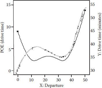
POE is a scary subject because it requires the use of mathematical tools that may be rusting at the back of your mind from long disuse. Although you can employ software (e.g., Design-Expert from Stat-Ease, Inc.) to do the “heavy lifting,” it may do you some good to do a light workout and tone up those math muscles. Fortunately, you’ve already developed a great deal of strength by learning how to make use of RSM for generating additive polynomial models that are extremely amenable to POE. For example, in Chapter 1, let’s revisit the model that we fit to the data collected on drive time:

${\displaystyle \widehat{\text{y}}}=32.1+1.7\text{x}-0.1{\text{x}}^2+0.00016{\text{x}}^3$

This equation is a cubic polynomial, which as you observed in Figure 1.11, creates a wavy surface that contains both highs and lows. We want to locate these plateaus and valleys because they represent points where variations in the input factors (x) transmit the least to the response (y). They can be pinpointed via POE.

The first step is calculation of the response variance $\left({\text{σ}}_{\text{y}}^{\text{2}}\right)$

${\text{σ}}_{\text{y}}^{\text{2}}={\left({\text{δ}}_{\text{y}}/{\text{δ}}_{\text{x}}\right)}^2{\text{σ}}_{\text{x}}^{\text{2}}+{\text{σ}}_{\text{e}}^{\text{2}}$

where ${\text{σ}}_{\text{x}}^{\text{2}}$ is the variance of the input factor x and ${\text{σ}}_{\text{e}}^{\text{2}}$ is the residual variance, which comes from the ANOVA. In the drive-time case, the standard deviation of Mark’s departure time is estimated to be 5 minutes; so, the values in the equation for variance are

${\text{σ}}_{\text{x}}^{\text{2}}={\left(5\text{minutes}\right)}^2=25$

${\text{σ}}_{\text{e}}^{\text{2}}=\text{Mean}\text{square}\text{residual}\text{from}\text{ANOVA}=5.18$

The partial derivative of the response y with respect to the factor x (δ_y/δ_x) for the drive-time model is

${\text{δ}}_{\text{y}}{\text{/δ}}_{\text{x}}=1.7-0.2\text{x}+0.00048{\text{x}}^2$

The POE is conveniently expressed in the original units of measure (minutes of drive time in this case) by taking the square root of the variance of response Y via this final equation:

$\begin{array}{lll}\text{POE}\hfill & =\hfill & \surd {\text{σ}}_{\text{y}}^{\text{2}}=\surd [{({\text{δ}}_{\text{y}}{\text{/δ}}_{\text{x}})}^2{\text{σ}}_{\text{x}}^{\text{2}}+{\text{σ}}_{\text{e}}^{\text{2}}]\hfill \\ \hfill & =\hfill & \surd [{(1.7-0.2\text{x}+0.00048{\text{x}}^2)}^2*25+5.18]\hfill \end{array}$

From here, it becomes “plug and chug” for those who enjoy doing oldfashioned hand calculations. However, with the aid of software, the POE can be more easily (and accurately!) calculated, mapped, and visualized. Figure 9.1 shows the POE for the drive-time case study. It exhibits two local minima, one for the peak at 11.5 (a high flat point in Figure 1.11) and one for the valley at 31.5 (a low flat point). (We superimposed a lightly shaded facsimile of the predicted drive time from Figure 1.11 on the POE pictured in Figure 9.1 to help you make the comparison.)

Figure 9.1  POE of drive time versus departure time.

Thus, POE finds two of the flats that are much desired by Six Sigma; so, life is good (so long as the commuter’s tires do not go flat!). As noted earlier, to conserve sleep, the commuter (Mark) chose the second minimum POE (31.5 minutes past 6:30 a.m., or a bit after 7 a.m.). Obviously, this implies that he gets in later to work. It turns out that Mark has the luxury of adjusting a second factor: flexible hours for the work day.

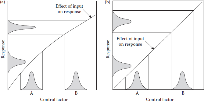
The commuting case illustrates an ideal system where factors affect the response in various ways:

  Nonlinear (departure time x)

  Linear (adjusting the work hours within a daily flex-time window)

Then, to reduce variability, the experimenter simply adjusts the nonlinear factor to minimize POE, and as a necessary follow-up, resets the linear factor to get the response back on target.

WHY POE BECOMES IRRELEVANT FOR LINEAR MODELS

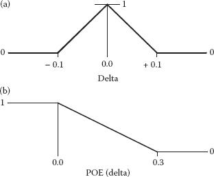
POE will be constant when the model is linear—it makes no difference where you set the factors: the variation transmitted does not change as shown in Figure 9.2b.

Therefore, linear factors can be freely adjusted to bring the response into specification while maintaining the gains made in reducing variation via POE on the nonlinear factors. In the case pictured above, take advantage of nonlinearity in response by setting the level of the first control factor (shown in Figure 9.2a) to reduce variation. Then, adjust the other factor (exhibiting the linear effect pictured in Figure 9.2b) to bring the response back to the desired set point.

Figure 9.2  (a) Variation transmitted via nonlinear responses. (b) Variation transmitted via linear responses.

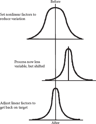
Figure 9.3 shows the ideal outcome for the application of POE—a big reduction in process variability, with no deleterious impact on the average response.

With information gained from POE analysis, the experimenter can adjust the nonlinear factors to minimize process variation. This tightens the distribution as shown by the middle curve in Figure 9.3. However, the average response now falls upon the target. Therefore, a linear factor must be adjusted to bring the process back into specification (the “after” curve). Thus, the mission of a robust design and Six Sigma is accomplished.

Figure 9.3  Before and after applying POE analysis.

An Application of POE for Three Factors Studied via a BBD

The drive-time example involves only one experimental factor. To get a better feel for the application of POE, let’s look at a more complex case study, one that involves three factors on a highly automated lathe (Anderson and Whitcomb, 1996). The data from a BBD are shown in Table 9.1. The response, labeled “Delta,” gives the deviation of the finished part’s dimension from its nominal value in mils (0.001 inches). Ideally, this delta can be stabilized at, or near, zero.

Regression analysis reveals a significant (p < 0.0001) quadratic model, shown below in terms of actual factors:

$\text{y}=1.42-0.00172\text{A}-98.4\text{B}-25.0\text{C}+0.235\text{AB}-0.0532\text{AC}+2.25*{10}^{-6}{\text{A}}^2+406{\text{C}}^2$

(Note: POE calculations, which we detail in Appendix 9A, operate on actual units of measure—not coded units.)

Table 9.1  Data from BBD on Lathe

Std	A: Speed (fpm)	B: Feed (ipr)	C: Depth (inches)	Y: Delta (mils)
1	330	0.01	0.075	0.0203
2	700	0.01	0.075	−0.357
3	330	0.022	0.075	−0.292
4	700	0.022	0.075	0.374
5	330	0.016	0.05	−0.394
6	700	0.016	0.05	0.227
7	330	0.016	0.1	0.572
8	700	0.016	0.1	0.208
9	515	0.01	0.05	−0.232
10	515	0.022	0.05	0.0886
11	515	0.01	0.1	0.123
12	515	0.022	0.1	0.471
13	515	0.016	0.075	−0.299
14	515	0.016	0.075	−0.183
15	515	0.016	0.075	−0.128
16	515	0.016	0.075	−0.146
17	515	0.016	0.075	−0.113

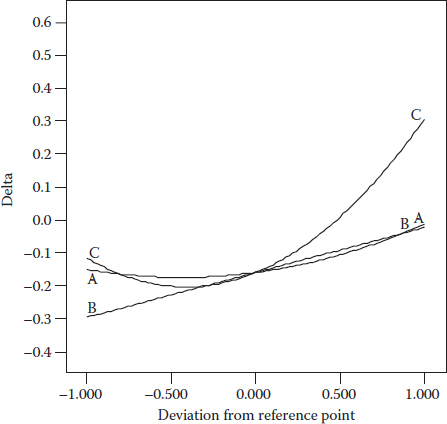
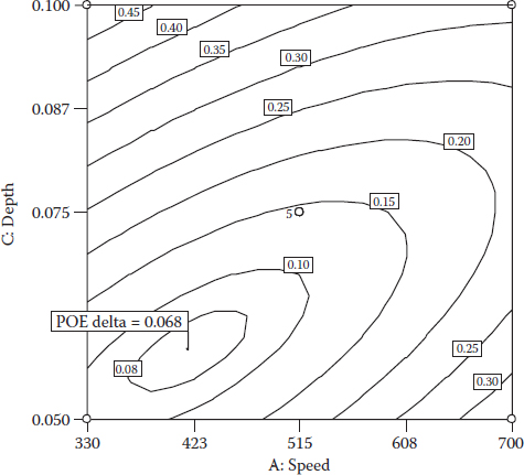
First, let’s explore the response surfaces generated by this model to see whether parts can be lathed to the proper dimension (delta equal to zero). Only two factors can be chosen for any given contour (or 3D) plot. Rather than choosing these arbitrarily, make use of the perturbation plot shown in Figure 9.4.

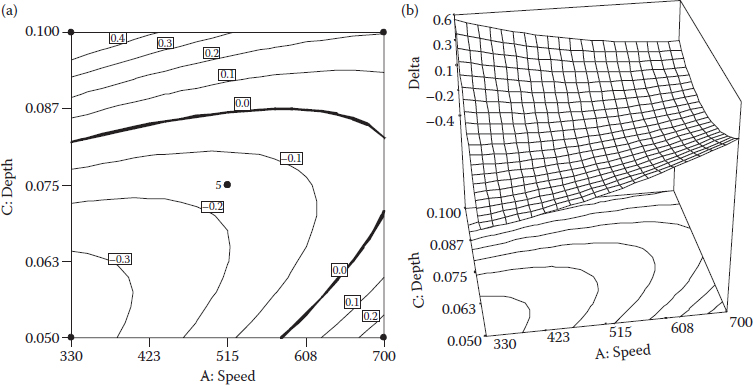
Notice that factor C (the depth of a cut) makes the most dramatic impact on the response, whereas B (the feed rate in inches per revolution) looks linear. Factor A (speed in feet per minute) falls somewhere in-between. Therefore, a plot of A versus C will be the most interesting (Figure 9.5a and b). We will keep B at its midpoint.

The 3D plot in Figure 9.5b reveals a flat-bottomed valley—an ideal place to locate the process for minimal POE. On the 2D plot in Figure 9.5a, we highlighted the ideal contour at zero delta. It is nice to know that, at this mid-level feed rate, the lathe operators can choose any number of combinations for speed and depth to achieve their part specification. However, let’s set the target aside for the moment and only concentrate on the calculation of the POE.

To compute POE, the variations in input factors must be specified as shown in Table 9.2. The relative variations are provided only for the sake of reference—to provide a feel on how well each factor can be controlled.

Figure 9.4  Perturbation plot of delta for the lathed part.

Figure 9.5  (a) 2D contour plots of speed versus depth. (b) 3D surface for delta.

For example, in this case, the depth (factor C) varied far more (25%) than speed (A—1.3%) on a relative basis. However, as one can infer from the broadly spaced contours, at certain locations, the response becomes insensitive to any variations in either of these two factors. To pinpoint this robust region, all we need to do is put the final piece of the puzzle into place—the standard deviation in response (provided from ANOVA by taking the square root of the mean square of the residual: 0.0675 mils). Then, the POE plot shown in Figure 9.6 can be generated.

It shows the most desirable location to be at the bottom end of both speed (A) and depth (C)—the lower-left quadrant in this experimental space. However, that cannot work because it will be put on the part that is off the target (i.e., delta will not be equal to zero). (Refer to Figure 9.5b to see this.) We must look out for a setting of factors that meets product specification at the minimum POE. This is just the sort of “less-filling/tastes great” multipleresponse conflict that we resolved in Chapter 6 by the use of the desirability function. In this case, we set the maximum desirability for delta at zero and POE minimized as shown in Figure 9.7a and b.

Table 9.2  Variation in Factors Affecting the Lathe

Factor	Test Limits	Range (Δ)	Standard Deviation (σ)	Relative Variation (σ/Δ) (%)
A: Speed (fpm)	330–700	370	5	1.3
B: Feed (ipr)	0.010–0.022	0.012	0.003	25
C: Depth (in.)	0.05–0.10	0.05	0.0125	25

Figure 9.6  POE contour plot.

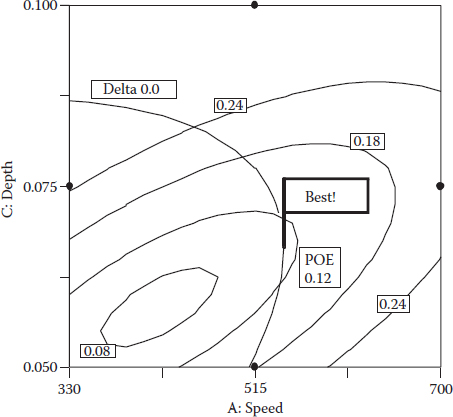
The threshold limits, where desirability drops to zero, are set somewhat arbitrarily in this case, but some slack must be allowed to facilitate the tradeoff between the demands of multiple responses. Table 9.3 shows the outcome of a numerical optimization on the overall desirability. (The POE is actually treated as a second response, y₂.)

Figure 9.7  (a) Desirability ramp for delta. (b) Desirability ramp for POE.

Table 9.3  Best Setup for the Lathe

Factor	Setting
A: Speed (fpm)	544
B: Feed (ipr)	0.022
C: Depth (in.)	0.067
y: Delta	0.00
POE (delta)	0.1

Figure 9.8  Best setup for the lathing product on spec consistently (feed maximized).

The manufacturing manager will like this outcome because it puts the feed rate at its maximum with product right on spec as consistently as possible—given the natural variations in inputs and the process as a whole. Figure 9.8 overlays contours for the delta and its POE with the best setup flagged.

It doesn’t get any better than this!

PRACTICE PROBLEMS

9.1  From the website for the program associated with this book, open the software tutorial titled “*Multifactor RSM*”.pdf (* signifies other characters in the file name) and page forward to Part 3. This is a direct follow-up to the tutorial that we directed you to in Problem 6.1, so, be sure to do that one (Part 2) first. This tutorial, which you should do now, demonstrates the use of the supplied software for doing POE. It requires the details on factor variation provided in Table 9.4.

Table 9.4  Standard Deviations in Input Factors

Factor	Test Limits	Range (Δ)	Standard Deviation (σ)	Relative Variation (σ/Δ) (%)
A: Time (minutes)	40–50	10	0.5	5
B: Temperature (deg C)	80–90	10	1	10
C: Catalyst (%)	2–3	1	0.05	5

This tutorial exercises a number of features in the software; so, if you plan to make use of this powerful tool, do not bypass it. However, even if you end up using a different software, you will still benefit by poring over the details on how to generate an operating setup that not only puts the process in its sweet spot relative to all specifications, but also at a point that will be most robust to variations transmitted from the input factors.

9.2  Consider the following standard deviations in the input factors for the DOE golfer discussed in Problem 8.2:

A.  Length, plus or minus 1 inch

B.  Angle, plus or minus 1 degree

C.  Weight, plus or minus 0.1 (assume that washers vary in weight)

There are many setups that achieve the goal of 72 inches, but will some of them result in less POE transmitted from these variations?

Appendix 9A: Details on How to Calculate POE

POE applied to RSM is done most efficiently with the aid of matrix algebra. The first step is a big one: do your DOE and fit an appropriate model to the response. Use the mean square of residuals from the ANOVA to estimate the underlying error variance $\left({\text{σ}}_{\text{e}}^{\text{2}}\right)$, and estimate the factor variances $\left({\text{σ}}_{\text{kk}}^{\text{2}}\right)$. Then proceed with POE as follows:

1.  Set up a matrix of factor variances:

${\text{σ}}_{\text{1}},{\text{σ}}_{\text{2}},\dots ,{\text{σ}}_{\text{k}}\Rightarrow \text{Σ}=\left(\begin{array}{lll}{\text{σ}}_{11}^2\hfill & 0\hfill & 0\hfill \\ 0\hfill & {\text{σ}}_{22}^2\hfill & 0\hfill \\ 0\hfill & 0\hfill & {\text{σ}}_{\text{kk}}^2\hfill \end{array}\right)$

2.  Calculate variance

$\text{Var}(\text{y})={\nabla }^{\text{T}}\text{Σ}\nabla +{\text{σ}}_{\text{e}}^{\text{2}}$

where

$\nabla =\left(\begin{array}{c}\frac{\partial \text{f}}{\partial {\text{x}}_1}\\ \frac{\partial \text{f}}{\partial {\text{x}}_2}\\ \frac{\partial \text{f}}{\partial {\text{x}}_{\text{k}}}\end{array}\right)$

$\begin{array}{l}\text{Var}(\text{y})=\left(\frac{\partial \text{f}}{\partial {\text{x}}_1}\frac{\partial \text{f}}{\partial {\text{x}}_2}\frac{\partial \text{f}}{\partial {\text{x}}_{\text{k}}}\right)\left(\begin{array}{lll}{\text{σ}}_{\text{11}}^{\text{2}}\hfill & \text{0}\hfill & \text{0}\hfill \\ \text{0}\hfill & {\text{σ}}_{\text{22}}^{\text{2}}\hfill & \text{0}\hfill \\ \text{0}\hfill & \text{0}\hfill & {\text{σ}}_{\text{kk}}^{\text{2}}\hfill \end{array}\right)\left(\begin{array}{c}\frac{\partial \text{f}}{\partial {\text{x}}_1}\\ \frac{\partial \text{f}}{\partial {\text{x}}_2}\\ \frac{\partial \text{f}}{\partial {\text{x}}_{\text{k}}}\end{array}\right)+{\text{σ}}_{\text{e}}^2\end{array}$

$\text{Var}(\text{y})={\left(\frac{\partial \text{f}}{\partial {\text{x}}_1}\right)}^2{\text{σ}}_{11}^2+\cdots +{\left(\frac{\partial \text{f}}{\partial {\text{x}}_{\text{k}}}\right)}^2{\text{σ}}_{\text{kk}}^2+{\text{σ}}_{\text{e}}^2$

3.  Complete the calculation for POE by taking the square root of the variance in response y:

$\text{POE}=\sqrt{\text{Var}(\text{y})}$

Some things to note about our calculations:

  All units of measure for factors are actual, and not coded.

  The POE is in the same units as the response measurements.

  They assume no covariance in the factors (all the off-diagonal elements in the matrix are zero); in other words, each factor’s noise is independent of all the other factors’ noise.

  They end at the second moment whereas others go on the third moment (Taylor, 1996), which produces a slightly higher result, but makes no difference for finding the flats—the ultimate objective for the application of POE to RSMs.

AN IMPORTANT CAVEAT ON POE

Up until now, we’ve always assumed that variation in the input factors (the x’s) will be constant regardless of their absolute level. For some factors, it may be more natural for the error in x to be a constant percent. In this case, the advantage of repositioning the factor in respect to the POE may be negated as shown in Figure 9A.1

Determining the variations in factors may prove to be the key for developing a valid prediction on POE. Do not assume that these will be constant across the operable ranges.

Figure 9A.1 Constant percent error for the input factor x.

POE for Transformed Responses

Occasionally, for statistical purposes, it becomes necessary to transform responses via mathematical functions such as the logarithm, square root, or the like (refer to DOE Simplified, Chapter 4: “Dealing with Non-Normality via Response Transformations”). Because RSM designs are geared to fit nonlinear surfaces, transformations are less likely to be beneficial than for screening studies via two-level factorials. That’s good because, as you will see, transformations create complications for the calculation of POE.

The transformed response, labeled y with a prime, is first fit to a polynomial function of the input factors (x’s) in the usual manner for RSMs. The POE in a transformed scale is then represented by

$\text{Var}({\text{y}}^{\prime })={\text{σ}}_{{\text{y}}^{\prime }}^2={\displaystyle {\displaystyle {\displaystyle \sum _{\text{i}=1}^{\text{k}}}}{\left(\frac{\partial {\text{y}}^{\prime }}{\partial {\text{x}}_{\text{i}}}\right)}^2{\text{σ}}_{{\text{x}}_{\text{i}}}^2+{\text{σ}}_{\text{resid}}^{\text{2}}}$

To get the response back into the original scale (y), the inverse of the transformation must be applied (e.g., an antilog on the logarithm). That’s simple compared to what’s needed to convert POE into the original scale—multiplication by the partial derivative of y with respect to y′ (δy/δy′) and application of the chain rule (from calculus):

$\frac{\partial \text{y}}{\partial \text{x}}=\frac{\partial \text{y}}{\partial {\text{y}}^{\prime }}\cdot \frac{\partial {\text{y}}^{\prime }}{\partial \text{x}}$

This yields

$\text{Var}(\text{y})={\text{σ}}_{\text{y}}^2={\displaystyle {\displaystyle \sum _{\text{i}=1}^{\text{k}}}{\left(\frac{\partial \text{y}}{\partial {\text{x}}_{\text{i}}}\right)}^2{\text{σ}}_{{\text{x}}_{\text{i}}}^2+{\left(\frac{\partial \text{y}}{\partial {\text{y}}^{\prime }}\right)}^2{\text{σ}}_{\text{resid}}^{\text{2}}}$

Finally, to compute the POE:

$\text{POE}=\sqrt{\text{Var}(\text{y})}$

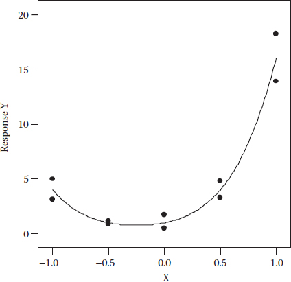
For example, assume that you do a simple one-factor RSM and collect the actual data as shown in Figure 9A.2. A good fit is accomplished with a quadratic model on the square root of the response.

Figure 9A.2 Data from one-factor RSM fitted to the square root of the response.

The model in transformed units (y′ = √y) is

${\text{y}}^{\prime }=1+1\text{x}+2{\text{x}}^2$

with a residual standard deviation (σ_resid) of 0.27.

The experimenter measures a standard deviation for the factor (σ_x) of 2.

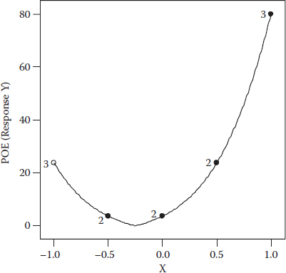
First, we calculate POE in the transformed scale

$\begin{array}{lll}\hfill {\text{σ}}_{{\text{y}}^{\prime }}^{\text{2}}& =\hfill & {\displaystyle {\displaystyle \sum _{\text{i}=1}^{\text{k}}}{\left(\frac{\partial {\text{y}}^{\prime }}{\partial \text{x}}\right)}^2{\text{σ}}_{\text{x}}^2+{\text{σ}}_{\text{resid}}^{\text{2}}}\hfill \\ \hfill \frac{\partial {\text{y}}^{\prime }}{\partial \text{x}}& =\hfill & \frac{\partial \left(1+1\text{x}+2{\text{x}}^2\right)}{\partial \text{x}}=1+4\text{x}\hfill \\ \hfill {\text{σ}}_{{\text{y}}^{\prime }}^2& =\hfill & {\left(1+4\text{x}\right)}^2{\left(2\right)}^2+{\left(0.27\right)}^2\hfill \\ \hfill {\text{POE}}_{{\text{y}}^{\prime }}& =\hfill & \sqrt{{\left(1+4\text{x}\right)}^2{\left(2\right)}^2+{\left(0.27\right)}^2}\hfill \end{array}$

Next, we convert the POE back into the original scale by multiplying ∂y/∂y′ and using the chain rule:

$\begin{array}{c}\frac{\partial \text{y}}{\partial \text{x}}=\frac{\partial \text{y}}{\partial {\text{y}}^{\prime }}\cdot \frac{\partial {\text{y}}^{\prime }}{\partial \text{x}}\\ \text{y}={\left({\text{y}}^{\prime }\right)}^2\therefore \frac{\partial \text{y}}{\partial {\text{y}}^{\prime }}=2\left({\text{y}}^{\prime }\right)\\ {\text{y}}^{\prime }=1+1\text{x}+2{\text{x}}^2\therefore \frac{\partial {\text{y}}^{\prime }}{\partial \text{x}}=1+4\text{x}\\ \frac{\partial \text{y}}{\partial \text{x}}=\frac{\partial \text{y}}{\partial {\text{y}}^{\prime }}\cdot \frac{\partial {\text{y}}^{\prime }}{\partial \text{x}}=2\left({\text{y}}^{\prime }\right)\cdot \left(1+4\text{x}\right)\\ {\text{σ}}_{\text{y}}^2={\left(\frac{\partial \text{y}}{\partial \text{x}}\right)}^2{\text{σ}}_{\text{x}}^2+{\left(\frac{\partial \text{y}}{\partial {\text{y}}^{\prime }}\right)}^2{\text{σ}}_{\text{resid}}^{\text{2}}\\ {\text{σ}}_{\text{y}}^2={\left(2\left({\text{y}}^{\prime }\right)\left(1+4\text{x}\right)\right)}^2{\text{σ}}_{\text{x}}^{\text{2}}+{\left(2\left({\text{y}}^{\prime }\right)\right)}^2{\text{σ}}_{\text{resid}}^{\text{2}}\\ \text{POE}=\sqrt{\left({\left(2\left(1+1\text{x}+2{\text{x}}^2\right)\left(1+4\text{x}\right)\right)}^2{\left(2\right)}^2+{\left(2\left(1+1\text{x}+2{\text{x}}^2\right)\right)}^2{\left(0.27\right)}^2\right)}\end{array}$

Wasn’t that fun? The plot of POE is shown in Figure 9A.3. When all is said and done, does this picture help you to locate the flats in the actual response?

Figure 9A.3 POE from a transformed response.

Yes, it does! Notice that the minimum in POE occurs where the response is the most stable (as seen in Figure 9A.2). This would be a good place to set the input factor x where its variation will be transmitted at the least—a goal consistent with the philosophy of Six Sigma.

“POE” NOT POE: FINAL THOUGHTS FOR THE MORE LITERARY READERS

POE is a very esoteric tool. For those who do not deal with numbers, it perhaps might be best described as “mathemagical.” Here’s a quote from the famous author of the same name (Poe). Did he disrespect statistics and calculus? You be the judge:

There are few persons, even among the calmest thinkers, who have not occasionally been startled into a vague yet thrilling half-credence in the supernatural, by coincidences of so seemingly marvelous a character that, as mere coincidences, the intellect has been unable to receive them … such sentiments are … thoroughly stifled by the doctrine of chance … technically termed the Calculus of Probabilities.

The Mystery of Marie Roget

A sequel to Poe’s more renowned novel

The Murders on the Rue Morgue