Chapter 19
Cisco DNA Software-Defined Access
This chapter examines one of Cisco’s newest and most exciting innovations in the area of enterprise networking—Software-Defined Access. SD-Access brings an entirely new way of building—even of thinking about and designing—the enterprise network. SD-Access embodies many of the key aspects of Cisco Digital Network Architecture, including such key attributes as automation, assurance, and integrated security capabilities.
However, to really appreciate what the SD-Access solution provides, we’ll first examine some of the key issues that confront enterprise network deployments today. The rest of the chapter presents the following:
Software-Defined Access as a fabric for the enterprise
Capabilities and benefits of Software-Defined Access
An SD-Access case study
The Challenges of Enterprise Networks Today
As capable as the enterprise network has become over the last 20-plus years, it faces some significant challenges and headwinds in terms of daily operation as well as present and future growth.
The enterprise network is the backbone of many organizations worldwide. Take away the network, and many companies, schools, hospitals, and other types of businesses would be unable to function. At the same time, the network is called upon to accommodate a vast and growing array of diverse user communities, device types, and demanding business applications.
The enterprise network continues to evolve to address these needs. However, at the same time, it also needs to meet an ever-growing set of additional—and critical—requirements. These include (but are not limited to) the need for:
Greater simplicity: Networks have grown to be very complicated to design, implement, and operate. As more functions are mapped onto the network, it must accommodate an ever-growing set of needs, and has become more and more complex as a result. Each function provided by the network makes sense in and of itself, but the aggregate of all the various functions, and their interaction, has become, for many organizations, cumbersome to implement and unwieldy to manage. Combined with the manually intensive methods typically used for network deployments, this complexity makes it difficult for the enterprise network to keep pace with the rate of change the organization desires, or demands.
Increased flexibility: Many enterprise network designs are relatively rigid and inflexible. The placement of Layer 2 and Layer 3 boundaries can, in some cases, make it difficult or impossible to accommodate necessary application requirements. For example, an application may need, or desire, a common IP subnet to be “stretched” across multiple wiring closets in a site. In a traditional routed access design model (in which IP routing is provisioned down to the access layer), this requirement is not possible to accommodate. In a multilayer design model, this need could be accommodated, but the use of a wide-spanning Layer 2 domain in this model (depending on how it is implemented) may expose the enterprise to the possibility of broadcast storms or other similar anomalies that could cripple the network. Organizations need their networks to be flexible to meet application demands such as these, when they arise. Today’s network designs often fall short. Although such protocols and applications can be altered over time to reduce or eliminate such requirements, many organizations face the challenge of accommodating such legacy applications and capabilities within their networks. Where such applications can be altered or updated, they should be—where they cannot be, a network-based solution may be advantageous.
Integrated security: Organizations depend on their networks. The simple fact is that today, the proper and ongoing operation of the network is critical to the functioning of any organization, and is foundational for the business applications used by that organization. Yet, many networks lack the inherent security and segmentation systems that may be desired. Being able to separate corporate users from guests, Internet of Things (IoT) devices from internal systems, or different user communities from each other over a common network has proved to be a daunting task for many enterprise networks in the past. Capabilities such as Multiprotocol Label Switching Virtual Private Networks (MPLS VPNs) exist, but are complex to understand, implement, and operationalize for many enterprise deployments.
Integrated mobility: The deployment and use of mobile, wireless devices is ubiquitous in today’s world—and the enterprise network is no exception. However, many organizations implement their wireless network separate from and “over the top” of their existing wired network, leading to a situation where the sets of available network services (such as security capabilities, segmentation, quality of service [QoS], etc.) are different for wired and wireless users. As a consequence, wired and wireless network deployments typically do not offer a simple, ubiquitous experience for both wired and wireless users, and typically cannot offer a common set of services with common deployment models and scale. As organizations move forward and embrace wireless mobile devices even further in their networks, there is a strong desire to provide a shared set of common services, deployed the same way, holistically for both wired and wireless users within the enterprise network.
Greater visibility: Enterprise networks are carrying more traffic, and more various types of traffic, across their network backbones than ever before. Being able to properly understand these traffic flows, optimize them, and plan for future network and application growth and change are key attributes for any organization. The foundation for such an understanding is greater visibility into what types of traffic and applications are flowing over the network, and how these applications are performing versus the key goals of the organization. Today, many enterprises lack the visibility they want into the flow and operation of various traffic types within their networks.
Increased performance: Finally, the ever-greater “need for speed” is a common fact of life in networking—and for the devices and applications they support. In the wired network, this includes the movement beyond 10-Gigabit Ethernet to embrace the new 25-Gbps and 100-Gbps Ethernet standards for backbone links, as well as multi-Gigabit Ethernet links to the desktop. In the wireless network, this includes the movement toward 802.11ac Wave 2 deployments, and in future the migration to the new 802.11ax standard as this emerges—all of which require more performance from the wired network supporting the wireless devices. By driving the performance per access point (AP) toward 10 Gbps, these developments necessitate a movement toward a distributed traffic-forwarding model, as traditional centralized forwarding wireless designs struggle to keep pace.
Cisco saw these trends, and others, beginning to emerge in the enterprise network space several years ago. In response, Cisco created Software-Defined Access (SD-Access). The following sections explore
A high-level review of SD-Access capabilities
What SD-Access is—details of architecture and components
How SD-Access operates: network designs, deployments, and protocols
The benefits that SD-Access provides, and the functionality it delivers
So, let’s get started and see what SD-Access has in store!
Software-Defined Access: A High-Level Overview
In 2017, Cisco introduced Software-Defined Access as a new solution that provides an automated, intent-driven, policy-based infrastructure with integrated network security and vastly simplified design, operation, and use.
SD-Access, at its core, is based on some of the key technologies outlined previously in this book:
Cisco DNA Center: Cisco DNA Center is the key network automation and assurance engine for SD-Access deployments. When deployed in conjunction with Cisco Identity Services Engine (ISE) as the nexus for policy and security, Cisco DNA Center provides a single, central point for the design, implementation, and ongoing maintenance and operation of an SD-Access network.
Cisco DNA flexible infrastructure: The flexible infrastructure of Cisco DNA was covered in depth in Chapter 7, “Hardware Innovations” and Chapter 8, “Software Innovations.” By levering these flexible, foundational hardware and software elements within a Cisco network, SD-Access is able to offer a set of solutions that allows an evolutionary approach to network design and implementation—easing the transition to the software-defined, intent-driven networking world, and providing outstanding investment protection.
Next-generation network control-plane, data-plane, and policy-plane capabilities: SD-Access builds on top of existing capabilities and standards, such as those outlined in Chapter 9, “Protocol Innovations,” including Location/ID Separation Protocol (LISP), Virtual Extensible Local Area Network (VXLAN), and Scalable Group Tags (SGT). By leveraging these capabilities, expanding upon them, and linking them with Cisco DNA Center to provide a powerful automation and assurance solution, SD-Access enables the transition to a simpler, more powerful, and more flexible network infrastructure for organizations of all sizes.
SD-Access: A Fabric for the Enterprise
The SD-Access solution allows for the creation of a fabric network deployment for enterprise networks. So, let’s begin with examining two important areas:
What is a fabric?
What benefits can a fabric network deployment help to deliver?
What Is a Fabric?
Effectively, a fabric network deployment implements an overlay network. Overlays by themselves are not new—overlay technologies of various flavors (such as CAPWAP, GRE, MPLS VPNs, and others) have been used for many years. Fundamentally, overlays leverage some type of packet encapsulation at the data plane level, along with a control plane to provision and manage the overlay. Overlays are so named because they “overlay,” or ride on top of, the underlying network (the underlay), leveraging their chosen data plane encapsulation for this purpose. Chapter 9 introduced overlays and fabrics in more detail, so this will serve as a refresher.
Figure 19-1 outlines the operation of an overlay network.
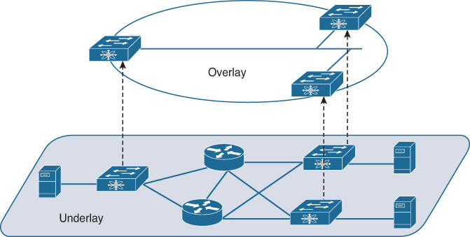
Overlay networks provide a logical, virtual topology for the deployment, operating on top of the physical underlay network. The two distinct “layers” of the network—logical and physical—can and often do implement different methods for reachability, traffic forwarding, segmentation, and other services within their respective domains.
A network fabric is the combination of the overlay network type chosen and the underlay network that supports it. But before we examine the type of network fabric created and used by SD-Access, we need to answer an obvious question: why use a fabric network at all for enterprise deployments?
Why Use a Fabric?
Perhaps the clearest way to outline why a fabric network is important within the enterprise is to quickly recap the main issues facing enterprise networks, namely:
The need for greater simplicity
The need for increased flexibility
The need for enhanced security
The requirement for ubiquitous mobility
The need for greater visibility
The need for simplified and more rapid deployment
And the ever-growing need for more performance
These various demands place network managers into an awkward position. As stewards of one of the most critical elements of an organization—the enterprise network—one of their primary tasks is to keep the network operational at all times: 24/7/365. How best to accomplish this is broken down into a few simple, high-level steps:
Step 1. Design the network using a solid approach.
Step 2. Implement that design using reliable, proven hardware and software, leveraging a best-practices deployment methodology.
Step 3. Implement a robust set of change-management controls, and make changes only when you must.
Essentially, this means “build the network right in the first place—then stand back and don’t touch it unless you need to.”
Although this approach is functional, it ignores the additional realities imposed upon network managers by other pressures in their organizations. The constant demand to integrate more functions into the enterprise network—voice, video, IoT, mission-critical applications, mergers and acquisitions, and many more—drives the need for constant churn in the network design and deployment. More virtual LANs (VLANs). More subnets. More access control lists (ACLs) and traffic filtering rules. And the list goes on.
In effect, many network managers end up getting pulled in two contradictory directions, as illustrated in Figure 19-2.

Essentially, many networks undergo this tension between these two goals: keep the network stable, predictable, and always on, and yet at the same time drive constant churn in available network services, functions, and deployments. In a network that consists of only one layer—essentially, that just consists of an underlay, as most networks do today—all of these changes have to be accommodated in the same physical network design and topology.
This places the network at potential risk with every design change or new service implementation, and explains why many organizations find it so slow to roll out new network services, such as (but not limited to) critical capabilities such as network-integrated security and segmentation. It’s all a balance of risk versus reward.
Networks have been built like this for many years. And yet, the ever-increasing pace of change and the need for new enhanced network services are making this approach increasingly untenable. Many network managers have heard these complaints from their organizations: “The network is too slow to change.” “The network is too inflexible.” “We need to be able to move faster and remove bottlenecks.”
So, how can a fabric deployment, using Software-Defined Access, help enterprises to address these concerns?
One of the primary benefits of a fabric-based approach is that it separates the “forwarding plane” of the network from the “services plane.” This is illustrated in Figure 19-3.
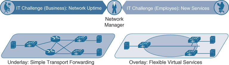
In this approach, the underlay provides the basic transport for the network. Into the underlay are mapped all of the network devices—switches and routers. The connectivity between these devices is provided using a fully routed network design, which provides the maximum stability and performance (using Equal Cost Multipath [ECMP] routing) and minimizes reconvergence times (via appropriate tuning of routing protocols). The underlay network is configured once and rarely if ever altered unless physical devices or links are added or removed, or unless software updates need to be applied. It is not necessary to make any changes to the underlay to add virtualized services for users. In a fabric-based design, the underlay provides the simple, stable, solid foundation that assists in providing the maximum uptime that organizations need from their network implementations.
The overlay, on the other hand, is where all of the users, devices, and things (collectively known as endpoints) within a fabric-based network are mapped into. The overlay supports virtualized services (such as segmentation) for endpoints, and supports constant change as new services and user communities are added and deleted. Changes to one area of the overlay (for example, adding a new virtual network, or a new group of users or devices) do not affect other portions of the overlay—thus helping to provide the flexibility that organizations require, without placing the network overall at risk.
In addition, because the overlay provides services for both wired and wireless users, and does so in a common way, it assists in creating a fully mobile workplace. With a fabric implementation, the same network services are provided for both wired and wireless endpoints, with the same capabilities and performance. Wired and wireless users alike can enjoy all of the virtualization, security, and segmentation services that a fabric deployment offers.
And speaking of security, an inherent property of a fabric deployment is network segmentation. As outlined in Chapter 9, next-generation encapsulation technologies such as VXLAN provide support for both virtual networks (VNs) and SGTs, allowing for both macro- and micro-segmentation. As you will see, these two levels of segmentation can be combined within SD-Access to provide an unprecedented level of network-integrated segmentation capabilities, which is very useful to augment network security.
Finally, a fabric deployment allows for simplification—one of the most important areas of focus for any organization. To find out why, let’s explore this area a bit further.
Networks tend to be very complex, in many cases due to the difficulty of rolling out network-wide policies such as security (ACLs), QoS, and the like. Many organizations use a combination of security ACLs and VLANs to implement network security policies—mapping users, devices, and things into VLANs (statically or dynamically), and then using ACLs on network devices or firewalls to implement the desired security policies. However, in the process of doing so, many such organizations find that their ACLs end up reflecting their entire IP subnetting structure—i.e., which users in which subnets are allowed to communicate to which devices or services in other subnets ends up being directly “written into” the ACLs the organization deploys.
If you recall, this was examined in some detail back in Chapter 9. The basic fact is that the IP header contains no explicit user/device identity information, so IP addresses and subnets are used as a proxy for this. However, this is how many organizations end up with hundreds, or even thousands, of VLANs. This is how those same organizations end up with ACLs that are hundreds or thousands of lines long—so long and complex, in fact, that they become very cumbersome to deploy, as well as difficult or impossible to maintain. This slows down network implementations, and possibly ends up compromising security due to unforeseen or undetected security holes—all driven by the complexity of this method of security operation.
A fabric solution offers a different, and better, approach. All endpoints connecting to a fabric-based network such as SD-Access are authenticated (either statically or dynamically). Following this authentication, they are assigned to a Scalable Group linked with their role, as well as being mapped into an associated virtual network. These two markings—SGT and VN—are then carried end to end in the fabric overlay packet header (using VXLAN), and all policies created within the fabric (i.e., which users have access to which resources) are based on this encoded group information—not on their IP address or subnet. The abstraction offered by the use of VNs and SGTs for grouping users and devices within an SD-Access deployment is key to the increased simplicity that SD-Access offers versus traditional approaches.
All packets carried within an SD-Access fabric contain user/device IP address information, but this is not used for applying policy in an SD-Access fabric. Polices within SD-Access are group-based in nature (and thus known as group-based policies, or GBPs). IP addresses in SD-Access are used for determining reachability (where has a host connected from or roamed to) as tracked by the fabric’s LISP control plane. Endpoints are subject to security and other policies based on their flexible groupings, using SGTs and VNs as their policy tags—tags that are carried end to end within the SD-Access fabric using the VXLAN-based overlay.
Now you are beginning to see the importance of the protocols—LISP, VXLAN, and SGTs—that were covered in Chapter 9. If you skipped over that section, it is highly recommended to go back and review it now. These protocols are the key to creating network fabrics, and to enabling the next generation of networking that SD-Access represents. They serve as the strong foundation for a fabric-enabled network—one that enables the simplicity and flexibility that today’s organizations require—while also providing integrated support for security and mobility, two key aspects of any modern network deployment.
Capabilities Offered by SD-Access
Now that you understand the power that the separation of IP addressing and policy offered by Software-Defined Access provides, let’s delve a bit deeper and see what advanced, next-generation, network-level capabilities SD-Access offers for organizations.
Virtual Networks
First and foremost, SD-Access offers macro-segmentation using VNs. Equivalent to virtual routing and forwarding instances (VRF) in a traditional segmentation environment, VNs provide separate routed “compartments” within the fabric network infrastructure. Users, devices, and things are mapped into the same, or different VNs, based on their identity. Between VNs, a default-deny policy is implemented (i.e., endpoints in one VN have no access to endpoints in another VN by default). In effect, VNs provide a first level of segmentation that, by default, ensures no communications between users and devices located in different VNs. This is illustrated in Figure 19-4.
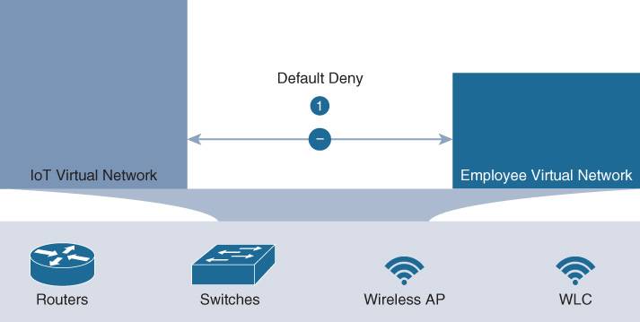
In this example, IoT devices are placed into one VN, and employees into another. Because the two VNs are separate and distinct routing spaces, no communication from one to the other is possible, unless explicitly permitted by the network administrator (typically via routing any such inter-VN traffic via a firewall, for example).
VNs provide a “macro” level of segmentation because they separate whole blocks of users and devices. There are many situations where this is desirable—examples include hospitals, airports, stadiums, banks…in fact, any organization that hosts multiple different types of users and things, and which needs these various communities sharing the common network infrastructure to be securely (and simply) separated from each other, while still having access to a common set of network services.
However, as useful as VNs are, they become even more powerful when augmented with micro-segmentation, which allows for group-based access controls even within a VN. Let’s explore this next.
Scalable Groups
The use of Scalable Groups within SD-Access provides the capability for intra-VN traffic filtering and control. Scalable Groups have two aspects: a Scalable Group Tag (SGT), which serves as the group identity for an endpoint, and which is carried end to end in the SD-Access fabric within the VXLAN fabric data plane encapsulation, and a Scalable Group ACL (SGACL, sometimes also previously known as Security Group ACL), which controls what other hosts and resources are accessible to that endpoint, based on the endpoint’s identity and role.
Group-based polices are far easier to define and understand than traditional IP-based ACLs because they are decoupled from the actual IP address structure in use. In this way, group-based ACLs are much more tightly aligned with the way that humans think about network security policies—“I want to give this group of users access to this, this, and this, and deny them from access to that and that”—and, as such, group-based policies are far easier to define, use, and understand than traditional access controls based on IP addresses and subnets.
Group-based policies are defined using either a whitelist model or a blacklist model. In a whitelist model, all traffic between groups is denied unless it is explicitly permitted (i.e., whitelisted) by a network administrator. In a blacklist model, the opposite is true: all traffic between groups is permitted unless such communication is explicitly blocked (i.e., blacklisted) by a network administrator.
In Software-Defined Access, a whitelist model is used by default for the macro-segmentation of traffic between VNs, and a blacklist model is used by default for the micro-segmentation of traffic between groups in the same VN. In effect, the use of groups within SD-Access provides a second level of segmentation, allowing the flexibility to control traffic flows at a group level even within a given VN.
The use of these two levels of segmentation provided by SD-Access—VNs and SGTs—is illustrated in Figure 19-5.
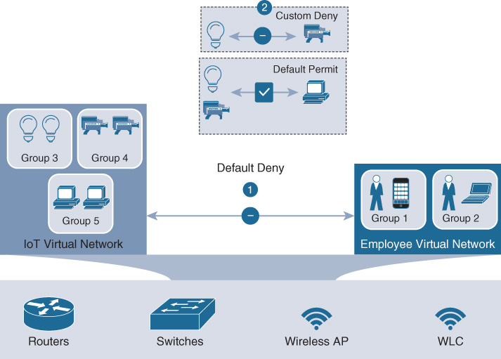
By providing two levels of segmentation, macro and micro, SD-Access provides the most secure network deployment possible for enterprises, and yet at the same time the simplest such approach for such organizations to understand, design, implement, and support. By including segmentation as an integral part of an SD-Access fabric deployment, SD-Access makes segmentation consumable—and opens up the power of integrated network security to all organizations, large and small.
Using Cisco DNA Center, SD-Access also makes the creation and deployment of VNs and group-based policies extremely simple. Policies in SD-Access are tied to user identities, not to subnets and IP addresses. After policies are defined, they seamlessly follow a user or device as it roams around the integrated wired/wireless SD-Access network. Policies are assigned simply by dragging and dropping groups in the Cisco DNA Center user interface, and are completely automated for deployment and use, as illustrated in Figure 19-6.
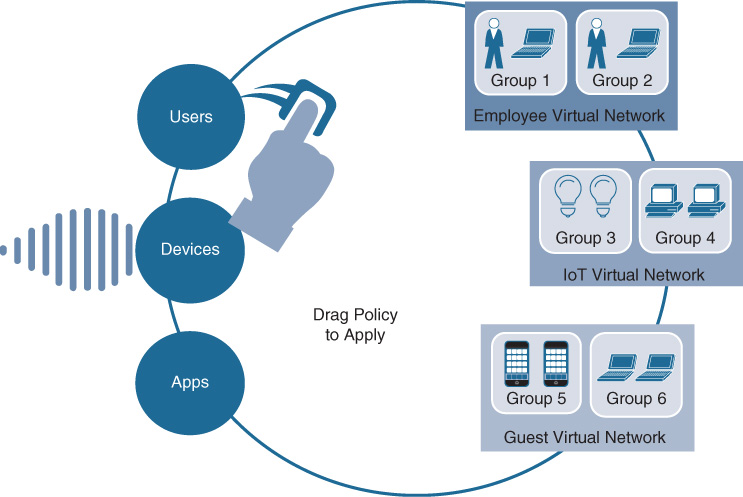
Before SD-Access, policies were VLAN and IP address based, requiring the network manager to create and maintain complex IP-based ACLs to define and enforce access policy, and then deal with any policy errors or violations manually. With SD-Access, there is no VLAN or IP address/subnet dependency for segmentation and access control (as these are defined at the VN/SGT grouping levels). The network manager in SD-Access is instead able to define one consistent policy, associated with the identity of the user or device, and have that identity (and the associated policy) follow the user or device as it roams within the fabric-based network infrastructure.
As you will see, policies within SD-Access are based on contracts that define who, or what, the user or device has access to in the network. Such contracts are easily updated via Cisco DNA Center to reflect new policy rules and updates as these change over time—with the resulting network-level policies then pushed out to the network elements involved in an automated fashion. This massively simplifies not only the initial definition of network policies, but also their ongoing maintenance over time.
In summary, simplified, multilevel network segmentation based on virtual networks and group-based policy is an inherent property of what SD-Access offers, and is an extremely important and powerful part of the solution.
Let’s continue on and explore what else SD-Access has in store.
Stretched Subnets
Most organizations at one time or another have faced the need to provide a single IP subnet that spans across—i.e., is “stretched between”—multiple wiring closets within a campus deployment. The reasons for such a need vary. They might involve applications that need to reside within a single common subnet, or older devices that cannot easily employ subnetting (due to the higher-level protocols they employ). Whatever the reason, such deployment requests pose a quandary for the typical network manager. Providing this capability in a traditional network deployment means extending a VLAN between multiple wiring closets—connecting them all together into a single, widely spanned Layer 2 domain. Although this is functional to meet the need, acceding to such requests places their network at overall risk.
Because all modern networks employ redundant interconnections between network devices, such wide-spanning Layer 2 domains create loops—many loops—in a typical enterprise network design. The Spanning Tree Protocol “breaks” any such loops by blocking ports and VLANs on redundant uplinks and downlinks within the network, thus avoiding the endless propagation of Layer 2 frames (which are not modified on forwarding) over such redundant paths.
However, this wastes much of the bandwidth (up to 50 percent) within the network due to all of the blocking ports in operation, and is complex to maintain because now there is a Layer 2 topology (maintained via Spanning Tree) and a Layer 3 topology (maintained via routing protocols and first-hop redundancy protocols) to manage, and these must be kept congruent to avoid various challenges to traffic forwarding and network operation. And even when all of this is done, and done properly, the network is still at risk because any misbehaving network device or flapping link could potentially destabilize the entire network—leading in the worst case to a broadcast storm should Spanning Tree fail to contain the issue.
Essentially, the use of wide-spanning Layer 2 VLANs places the entire network domain over which they span into a single, common failure domain—in the sense that a single failure within that domain has the potential to take all of the domain down, with potentially huge consequences for the organization involved.
Due to these severe limitations, many network managers either ban the use of wide-spanning VLANs entirely in their network topologies or, if forced to use them due to the necessity to deploy the applications involved, employ them gingerly and with a keen awareness of the ongoing operational risk they pose.
One of the major benefits provided by SD-Access, in addition to integrated identity-based policy and segmentation, is the ability to “stretch” subnets between wiring closets in a campus or branch deployment in a simple manner, and without having to pay the “Spanning Tree tax” associated with the traditional wide-spanning VLAN approach.
Figure 19-7 illustrates the use of stretched subnets within SD-Access.
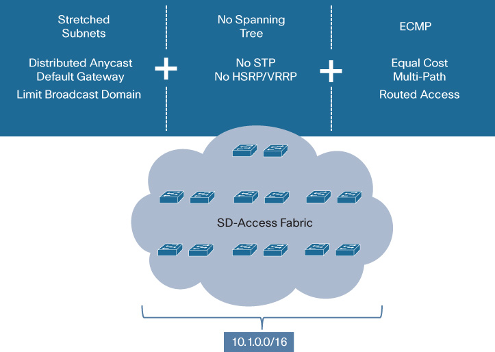
With SD-Access, a single subnet (10.1.0.0/16, as shown in Figure 19-7) is stretched across all of the wiring closets within the fabric deployment. By doing so, any endpoint attached within any of these wiring closets can (if properly authenticated) be mapped into this single, wide-spanning IP subnet, which appears identical to the endpoint (same default gateway IP and MAC address), regardless of where the endpoint is attached—without having to span Layer 2 across all of these wiring closets to provide this capability.
This is accomplished by the use of the Distributed Anycast Default Gateway function within SD-Access. No matter where a device attaches to the subnet shown, its default gateway for that subnet is always local, being hosted on the first-hop switch (hence, distributed). Moreover, it always employs the same virtual MAC address for this default gateway (thus, anycast). The combination of these two attributes makes the SD-Access fabric “look the same” no matter where a device attaches—a critical consideration for roaming devices, and a major factor in driving simplification of the network deployment.
In addition, it is vital to note that SD-Access provides this stretched subnet capability without actually extending the Layer 2 domain between wiring closets. Spanning Tree still exists southbound (i.e., toward user ports) from the wiring closet switches in an SD-Access deployment—but critically, Spanning Tree and the Layer 2 domain are not extended “northbound” across the SD-Access fabric. SD-Access makes it possible to have the same IP subnet appear across multiple wiring closets, without having to create Layer 2 loops as a traditional wide-spanning VLAN approach does.
In this way, SD-Access provides the benefits of a stretched IP subnet for applications and devices that may need this capability, but eliminates the risk otherwise associated with doing so. Broadcast domains are limited in extent to a single wiring closet, and no cross-network Layer 2 loops are created.
SD-Access also provides several additional key attributes with the approach it employs for stretched subnets.
First, because SD-Access instantiates the default gateway for each fabric subnet always at the first-hop network switch, traditional first-hop gateway redundancy protocols such as Hot Standby Router Protocol (HSRP) or Virtual Router Redundancy Protocol (VRRP) are not required. This eliminates a major level of complexity for redundant network designs, especially because maintaining congruity between the Layer 2 and Layer 3 first-hop infrastructures—a significant task in traditional networks—is not needed. SD-Access stretched subnets are very simple to design and maintain. In fact, all subnets (known as IP host pools) that are deployed within an SD-Access fabric site are stretched to all wiring closets within that fabric site by default.
Secondly, since SD-Access is deployed on top of a fully routed underlay network, ECMP routing is provided across the fabric for the encapsulated overlay traffic. This ensures that all links between switches in the fabric network are fully utilized—no ports are ever placed into blocking mode—offering vastly improved traffic forwarding compared to traditional Layer 2/Layer 3 designs.
To ensure that traffic is load-balanced over multiple paths optimally, the inner (encapsulated) endpoint packet’s IP five-tuple information (source IP, destination IP, source port, destination port, and protocol) is hashed into the outer encapsulating (VXLAN) packets’ source port. This ensures that all links are utilized equally within the fabric backbone by providing this level of entropy for ECMP link load sharing, while also ensuring that any individual flow transits over only one set of links, thus avoiding out-of-order packet delivery.
The use of a routed underlay also ensures rapid recovery in the event of network link or node failures, because such recovery takes place at the rapid pace associated with a routing protocol, not the relatively more torpid pace associated with Layer 2 reconvergence.
The use of a routed underlay for SD-Access results in a more stable, predictable, and optimized forwarding platform for use by the overlay network, and the ability to then deploy stretched subnets in the SD-Access overlay network provides a flexible deployment model without the trade-offs (i.e., inability to deploy a stretched-subnet design) that such a fully routed network deployment incurs in a traditional (non-fabric) network system.
Finally, the use of stretched subnets with SD-Access allows organizations to massively simplify their IP address planning and provisioning. Because subnets within the SD-Access fabric site are by default stretched to all wiring closets spanned by that fabric site, a much smaller number of much larger IP address pools can be provisioned and used for the site involved. This not only greatly simplifies an organization’s IP address planning, it leads to much more efficient use of the IP address pool space than the typical larger-number-of-smaller-subnets approach used by many enterprise network deployments. This simplicity and efficient use of IP address space in turn allows organizations to be speedier to adapt to the support of new devices and services that need to be mapped into the network infrastructure.
Now that we’ve examined some of the key network-level benefits of an SD-Access deployment, let’s continue and explore the components that combine to create an SD-Access solution.
SD-Access High-Level Architecture and Attributes
This section reviews the high-level architecture of SD-Access, outlines some of the major components that make up the solution, and examines the various attributes associated with these components.
SD-Access as a solution is composed of several primary building blocks:
Cisco DNA Center: This serves as the key component for implementation of the automation and assurance capabilities of SD-Access. Consisting physically of one or more appliances, Cisco DNA Center provides the platform from which an SD-Access solution is designed, provisioned, monitored, and maintained. Cisco DNA Center provides not only the design and automation capabilities to roll out an SD-Access fabric network deployment, it also provides the analytics platform functionality necessary to absorb telemetry from the SD-Access network, and provide actionable insights based on this network data.
Identity Services Engine: ISE provides a key security platform for integration of user/device identity into the SD-Access network. ISE allows for the policy and segmentation capabilities of SD-Access to be based around endpoint and group identity, allowing the implementation of network-based policies that are decoupled from IP addressing—a key attribute of an SD-Access deployment.
Network infrastructure (wired and wireless): The SD-Access solution encompasses both wired and wireless network elements, and provides the ability to create a seamless network fabric from these components. A review of which network elements make up an SD-Access fabric is outlined later in this chapter. A unique and powerful capability of SD-Access is the capacity to reuse many existing network infrastructure elements—switches, routers, access points, and Wireless LAN Controller (WLCs)—and repurpose them for use in a powerful new fabric-based deployment model.
By delivering a solution that embodies the best aspects of software flexibility and rapid development, with hardware-based performance and scale, SD-Access provides “networking at the speed of software.”
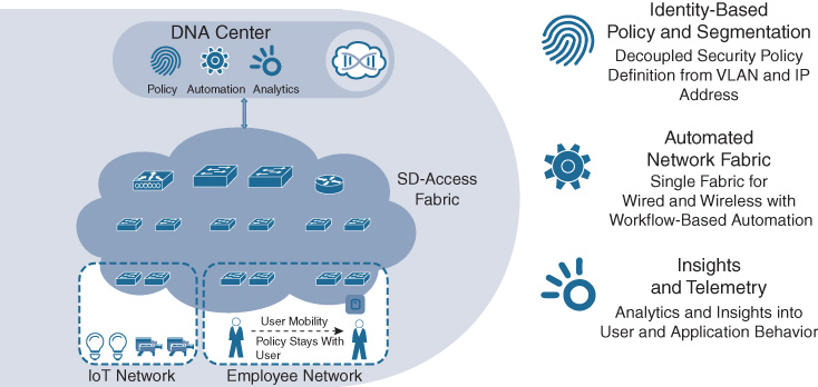
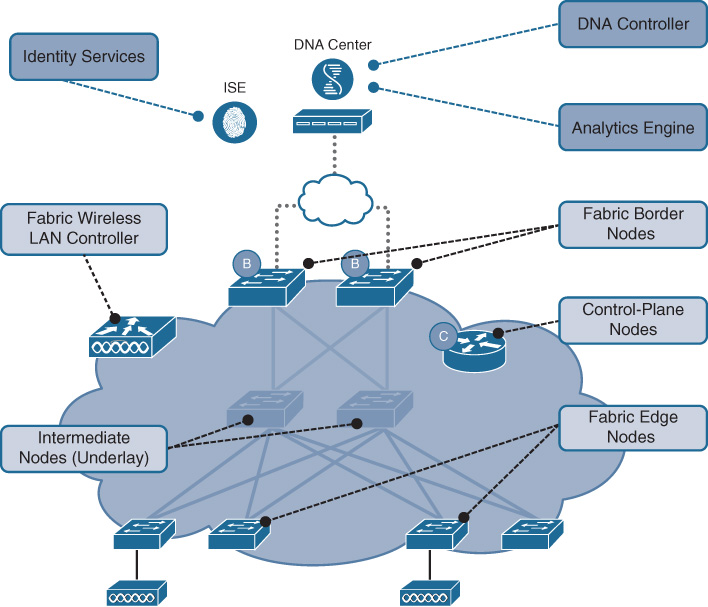
The high-level design of an SD-Access solution is shown in Figure 19-8, along with callouts concerning some of the key attributes of SD-Access.
Now, let’s dive into the details and examine how SD-Access is built, review the components that are part of an SD-Access solution, and detail the benefits SD-Access delivers.
SD-Access Building Blocks
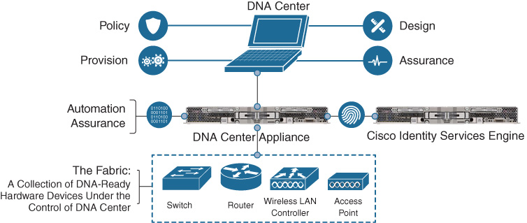
As mentioned, the SD-Access solution leverages several key building blocks: namely, Cisco DNA Center, ISE, and the network infrastructure elements which form the SD-Access fabric. Figure 19-9 illustrates these key building blocks of SD-Access:
Let’s begin by examining Cisco DNA Center, with a focus on how this supports an SD-Access deployment.
Cisco DNA Center in SD-Access
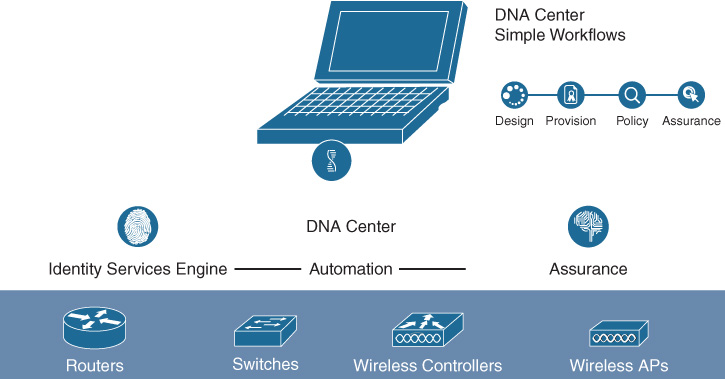
Cisco DNA Center’s support of the SD-Access solution set is focused on a four-step workflow model. These four major workflows consist of Design, Policy, Provision, and Assurance. The major focus of each of these four workflows is as follows:
Design: This workflow allows for the design of the overall system. This is where common attributes such as major network capabilities (DHCP and DNS services, IP host pools for user/device IP addressing, etc) are created and enumerated, as well as where network locations, floors, and maps are laid out and populated.
Policy: This workflow allows the creation of fabric-wide policies, such as the creation of Virtual Networks, Scalable Groups, and contracts between groups defining access rights and attributes, in line with defined organizational policies and goals.
Provision: Design and policy come together in this workflow, where the actual network fabrics are created, devices are assigned to various roles within those fabrics, and device configurations are created and pushed out to the network elements that make up the SD-Access overlay/underlay infrastructure.
Assurance: The final workflow allows for the definition and gathering of telemetry from the underlying network, with the goal of analyzing the vast amounts of data which can be gathered from the network and refining this into actionable insights.
These four workflows in Cisco DNA Center are outlined in Figure 19-10.
As the central point for defining, deploying, and monitoring the SD-Access network, Cisco DNA Center plays a key role in any SD-Access implementation. A single Cisco DNA Center instance can be used to deploy multiple SD-Access fabrics.
Many of the key attributes and capabilities of Cisco DNA Center were outlined previously as we examined the Automation and Assurance functionality of Cisco DNA. Any SD-Access deployment leverages Cisco DNA Center as the core element for the definition, management, and monitoring of the SD-Access fabric.
Now, let’s examine a few of the key elements that Cisco DNA Center provisions in an SD-Access fabric deployment.
SD-Access Fabric Capabilities
Three of these key elements which are defined in Cisco DNA Center and then rolled out into the SD-Access fabric for deployment are IP Host Pools, Virtual Networks, and Scalable Groups. Let’s double-click on each of these areas to gain a better understanding of the role they play in an SD-Access implementation.
IP Host Pools
IP host pools are created within Cisco DNA Center, and are the IP subnets which are deployed for use by users, devices, and things attached to the SD-Access fabric. Host pools, once defined within a fabric deployment, are bound to a given Virtual Network, and are rolled out by Cisco DNA Center to all of the Fabric Edge switches in the fabric site involved. The subnets defined in the Host Pools are rolled out onto all the network edge switches within that fabric site (same virtual IP and virtual MAC at all locations at that site), thus driving network simplification and standardization.
Each IP host pool is associated with a distributed anycast default gateway (as discussed previously) for the subnet involved, meaning that each edge switch in the fabric serves as the local default gateway for any endpoints (wired or wireless) attached to that switch. The given subnet is by default “stretched” across all of the edge switches within the given fabric site deployment, making this host pool available to endpoints no matter where they attach to the given fabric at that site.
Figure 19-11 illustrates the deployment and use of IP host pools within an SD-Access fabric deployment.
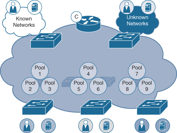
Endpoints attaching to the SD-Access fabric are mapped into the appropriate IP host pools, either statically, or dynamically based on user/device authentication, and are tracked by the fabric control plane, as outlined in the following text concerning fabric device roles. To provide simplicity and allow for easy host mobility, the fabric edge nodes that the endpoints attach to implement the distributed anycast default gateway capability, as outlined previously, providing a very easy-to-use deployment model.
Virtual Networks
Virtual networks are created within Cisco DNA Center and offer a secure, compartmentalized form of macro-segmentation for access control. VNs are mapped to VRFs, which provide complete address space separation between VNs, and are carried across the fabric network as virtual network IDs (VNIs, also sometimes referred to as VNIDs) mapped into the VXLAN data plane header.
An illustration of VNs within an SD-Access deployment is shown in Figure 19-12.
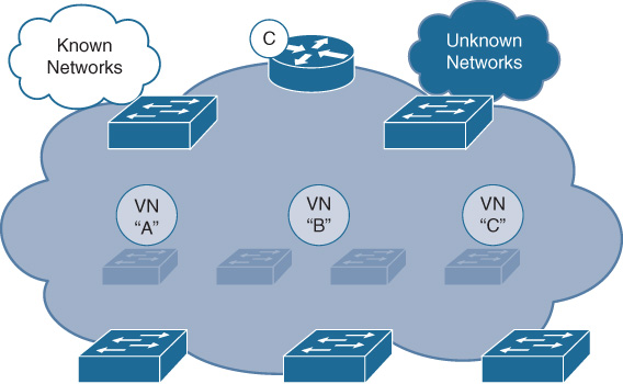
Every SD-Access fabric deployment contains a “default” VN, into which devices and users are mapped by default (i.e., if no other policies or mappings are applied). Additional VNs are created and used as desired by the network administrator to define and enforce the network segmentation polices that the administrator may wish to use within the SD-Access fabric. An additional VN that exists by default within an SD-Access deployment is the INFRA_VN (Infrastructure VN), into which network infrastructure devices such as access points and extended node switches are mapped.
The scale for implementation of additional VNs depends of the scalability associated with network elements within the fabric, including the border and edge node types involved. New platforms are introduced periodically, each with its own scaling parameters, and as well the scale associated with devices may also vary by software release. Please refer to Cisco.com, as well as resources such as the Software-Defined Access Design Guide outlined in the “Further Reading” section at the end of this chapter (https://www.cisco.com/c/dam/en/us/td/docs/solutions/CVD/Campus/CVD-Software-Defined-Access-Design-Guide-2018AUG.pdf) for the latest information associated with VN scale across various device types within an SD-Access fabric deployment.
Scalable Groups
Scalable Groups (SG) are created within Cisco DNA Center as well as ISE, and offer a secure form of micro-segmentation for access control. SGs are carried across the SD-Access fabric as SGTs mapped into the VXLAN data plane header. Scalable Group ACLs (SGACLs) are used for egress traffic filtering and access control with an SD-Access deployment, enforced at the fabric edge and/or fabric border positions in the fabric.
For additional details on the use the SGTs and SGACLs, please refer to Chapter 9, where this is covered in greater depth.
The use of SGTs within an SD-Access deployment is illustrated in Figure 19-13.
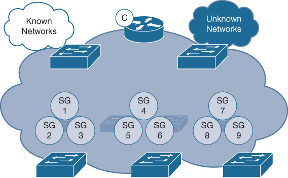
The combination of VNs and SGTs within the SD-Access solution, along with the automated deployment of these capabilities by Cisco DNA Center, provide an extremely flexible and powerful segmentation solution for use by enterprise networks of all sizes.
The ability to easily define, roll out, and support an enterprise-wide segmentation solution has long been a desirable goal for many organizations. However, it has often proved to be out of reach for many in the past due to the complexities (MPLS VPNs, VRF-lite, etc.) associated with previous segmentation solutions.
SD-Access and Cisco DNA Center now bring this powerful capability for two levels of segmentation—macro-segmentation using VNs, and micro-segmentation using SGTs—to many enterprise networks worldwide, making this important set of security and access control capabilities far more consumable than they were previously.
Now that you’ve been introduced to some of the higher-level constructs that Cisco DNA Center assists in provisioning in an SD-Access fabric deployment—IP host pools, virtual networks, and Scalable Groups—let’s delve into the roles that various network infrastructure devices support within the fabric.
SD-Access Device Roles
Various network infrastructure devices perform different roles within an SD-Access deployment, and work together to make up the network fabric that SD-Access implements.
The various roles for network elements with an SD-Access solution are outlined in Figure 19-14.
These various device roles and capabilities are summarized briefly as follows:
Cisco DNA Center: Serves as the overall element for designing, provisioning, and monitoring the SD-Access deployment, as well as for providing network monitoring and assurance capabilities.
Identity Services Engine: Serves as the primary repository for identity and policy within the SD-access deployment, providing dynamic authentication and authorization for endpoints attaching to the fabric. ISE also interfaces with external identity sources such as Active Directory.
Control plane nodes: One or more network elements that implement the LISP Map Server/Map Resolver (MS/MR) functionality. Basically, the control plane nodes within the SD-Access fabric “keep track” of where all the users, devices, and things attached to the fabric are located, for both wired and wireless endpoints. The control plane nodes are key elements within the SD-Access fabric architecture, as they serve as the “single source of truth” as to where all devices attached to the SD-Access fabric are located as they connect, authenticate, and roam.
Border nodes: One or more network elements that connect the SD-Access fabric to the “rest of the world” outside of the fabric deployment. One of the major tasks of the border node or nodes is to provide reachability in and out of the fabric environment, and to translate between fabric constructs such as virtual networks and Scalable Group Tags and the corresponding constructs outside of the fabric environment.
Edge nodes: Network elements (typically, many) that attach end devices such as PCs, phones, cameras, and many other types of systems into the SD-Access fabric deployment. Edge nodes serve as the “first-hop” devices for attachment of endpoints into the fabric, and are responsible for device connectivity and policy enforcement. Edge nodes in the LISP parlance are sometimes known as Routing Locators (RLOCs), and the endpoints themselves are denoted by Endpoint IDs (EIDs), typically IP addresses or MAC addresses.
Fabric Wireless LAN Controller (WLC): Performs all the tasks that the WLC traditionally is responsible for—controlling access points attached to the network and managing the radio frequency (RF) space used by these APs, as well as authenticating wireless clients and managing wireless roaming—but also interfaces with the fabric’s control plane node(s) to provide a constantly up-to-date map of which RLOCs (i.e., access-layer fabric edge switches) any wireless EIDs are located behind as they attach and roam within the wireless network.
Intermediate nodes: Any network infrastructure devices that are part of the fabric that lies “in between” two other SD-Access fabric nodes. In most deployments, intermediate nodes consist of distribution or core switches. In many ways, the intermediate nodes have the simplest task of all, as they are provisioned purely in the network underlay and do not participate in the VXLAN-based overlay network directly. As such, they are forwarding packets solely based on the outer IP address in the VXLAN header’s UDP encapsulation, and are often selected for their speed, robustness, and ability to be automated by Cisco DNA Center for this role.
It is important to note that any SD-Access fabric site must consist of a minimum of three logical components: at least one fabric control plane, one or more edges, and one or more borders. Taken together, these constructs comprise an SD-Access fabric, along with Cisco DNA Center for automation and assurance and ISE for authentication, authorization, and accounting (AAA) and policy capabilities.
Now, let’s explore a few of these device roles in greater detail to examine what they entail and the functions they perform. As we examine each role, a sample overview of which devices might typically be employed in these roles is provided.
SD-Access Control Plane Nodes, a Closer Look
The role of the control plane node in SD-Access is a crucial one. The control plane node implements the LISP MS/MR functionality, and as such is tasked with operating as the single source of truth about where all users, devices, and things are located (i.e., which RLOC they are located behind) as these endpoints attach to the fabric, and as they roam.
The SD-Access control plane node tracks key information about each EID and provides it on demand to any network element that requires this information (typically, to forward packets to that device’s attached RLOC, via the VXLAN overlay network).
Figure 9-15 illustrates the fabric control plane node in SD-Access.
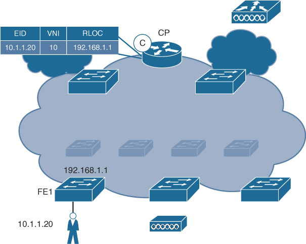
The fabric control plane node provides several important functions in an SD-Access network:
Acts as a host database, tracking the relationship of EIDs to edge node (RLOC) bindings. The fabric control plane node supports multiple different types of EIDs, such as IPv4 /32s and MAC addresses.
Receives prefix registrations from edge nodes for wired clients, and from fabric-mode WLCs for wireless clients.
Resolves lookup requests from edge and border nodes to locate endpoints within the fabric (i.e., which RLOC is a given endpoint attached to and reachable via).
Updates both edge and border nodes with wireless client mobility and RLOC information as clients roam within the fabric network system, as required.
Effectively, the control plane node in SD-Access acts as a constantly updated database for EID reachability. More than one control plane node can be (and would in most cases be recommended to be) deployed in an SD-Access fabric build.
If more than one control plane node is employed, they do not require or use any complex protocol to synchronize with each other. Rather, each control plane node is simply updated by all of the network elements separately—i.e., if two control plane nodes exist in a given fabric, an edge node, border node, or WLC attached to that fabric is simply configured to communicate with both control plane nodes, and updates both of them when any new device attaches to the fabric, or roams within it. In this way, the control plane node implementation is kept simple, without the complexity that would otherwise be introduced by state sync between nodes.
It is important to note that the control plane node is updated directly by an edge node (for example, an access switch) for wired clients attached to that switch, while for wireless clients the WLC (which manages the wireless domain) is responsible for interfacing with, and updating, the control plane node for wireless clients. The integration of wireless into an SD-Access fabric environment is examined in more detail later in this chapter.
A key attribute that it is critical to note about LISP as a protocol is that it is based on the concept of “conversational learning”—that is to say, a given LISP-speaking device (source RLOC) does not actually learn the location of a given EID (i.e., which destination RLOC that EID currently resides behind) until it has traffic to deliver to that EID. This capability for conversational learning is absolutely key to the LISP architecture, and is a major reason why LISP was selected as the reachability protocol of choice for SD-Access.
The task of a traditional routing protocol, such as Border Gateway Protocol (BGP), is essentially to flood all reachability information everywhere (i.e., to every node in the routing domain). Although this is workable when the number of reachability information elements (i.e., routes) is small—say, a few thousand—such an approach rapidly becomes impractical in a larger deployment.
Imagine, for example, a large campus such as a university that hosts on a daily basis (say) 50,000 to 75,000 users, each of whom may be carrying two or three network devices on average. Using an approach with a traditional routing protocol that attempted to flood the information about 150,000 to 200,000+ endpoints to all network devices would present a huge scaling challenge. Device ternary content-addressable memories (TCAMs) and routing tables would need to be enormous, and very expensive, and tracking all the changes as devices roamed about using the flooding-oriented control plane approach of a traditional routing protocol would rapidly overwhelm the CPU resource available even in large routing platforms—let alone the relatively much smaller CPU and memory resources available in (say) an access switch at the edge of the network.
Rather than use this approach, the LISP control plane node, operating in conjunction with LISP-speaking devices such as edge and border nodes, provides a conversational learning approach where the edge and border nodes query the control plane node for the destination RLOC to use when presented with traffic for a new destination (i.e., one that they have not recently forwarded traffic for). The edges and borders then cache this data for future use, reducing the load on the control plane node.
This use of conversational learning is a major benefit of LISP, as it allows for massive scalability while constraining the need for device resources, and is one of the major motivations for the use of LISP as the control plane protocol for use in SD-Access.
For further details on the operation of LISP, please refer to Chapter 9, which provides a description of the LISP protocol itself, as well as how roaming is handled within LISP.
SD-Access Control Plane Nodes: Supported Devices
Multiple devices can fulfill the task of operating as a fabric control plane node. The selection of the appropriate device for this critical task within the fabric is largely based on scale—in terms of both the number of EIDs supported and the responsiveness and performance of the control plane node itself (based on CPU sizing, memory, and other control plane performance factors).
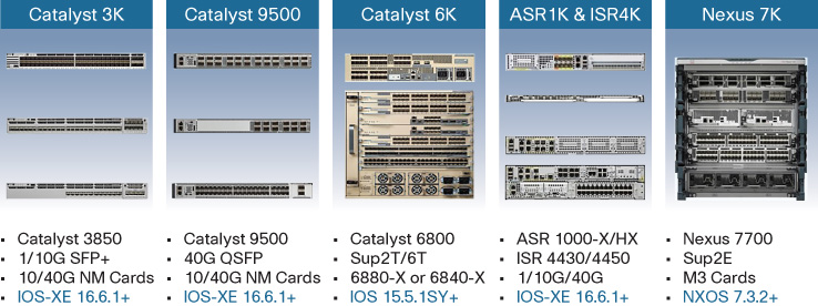
Figure 19-16 outlines some of the platforms that, as of this writing, are able to operate as control plane nodes within the SD-Access fabric.
For many deployments, the fabric control plane node function is based on a switch platform. This is often very convenient, as such switches often exist in the deployment build in any case.
The control plane function is either co-located on a single device with the fabric border function (outlined in the following section) or implemented on a dedicated device for the control plane node. Typically, dedicating a device or devices to the control plane role, rather than having them serve dual functions, results in greater scalability as well as improved fault tolerance (because a single device failure then only impacts one fabric role/function, not both simultaneously). Nevertheless, many fabrics may choose to implement a co-located fabric control plane/border node set of functions on a common device, for the convenience and cost savings this offers.
Typically, the Catalyst 3850 platform (fiber based) is selected as a control plane node only for the smallest fabric deployments, or for pilot systems where an SD-Access fabric is first being tested. The amount of memory and CPU horsepower available in the Catalyst 3850 significantly restricts the scalability it offers for this role, however.
Many fabric deployments choose to leverage a Catalyst 9500 switch as a fabric control plane node. The multicore Intel CPU used in these platforms provides a significant level of performance and scalability for such fabric control plane use, and makes the Catalyst 9500 an ideal choice for many fabric control plane deployments. For branch deployments that require a fabric control plane, the ISR 4000 platforms are also leveraged for this task, with their CPU and memory footprint making them well suited to this task for a typical branch.
The very largest fabric deployments may choose to leverage an ASR 1000 as a fabric control plane node. This offers the greatest scalability for those SD-Access fabric installations that require it. It is worth noting that some control plane node types offer more limited functionality than others.
Please refer to Cisco.com, as well as resources such as the Software-Defined Access Design Guide outlined in the “Further Reading” section at the end of this chapter, for the exact details of the scalability and functionality for each of these control plane options, which vary between platform types. The control plane scale associated with these platforms may also vary between software releases, so referring to the latest online information for these scaling parameters is recommended.
Because new platforms are always being created, and older ones retired, please also be sure to refer to Cisco.com for the latest information on supported devices for the SD-Access fabric control plane role.
SD-Access Fabric Border Nodes, a Closer Look
Now, let’s examine further the role of a fabric border node in SD-Access fabric.
As previously mentioned, the task of a border node is twofold: to connect the SD-Access fabric to the outside world, and to translate between SD-Access fabric constructs (VNs, SGTs) and any corresponding constructs in the outside network.
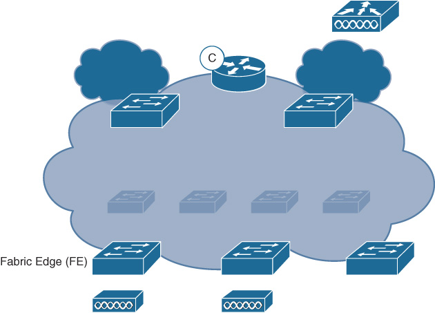
Figure 19-17 depicts fabric border nodes (marked with a B) in an SD-Access deployment.
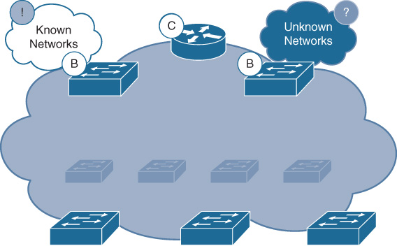
An important item to note is that SD-Access defines two basic types of border node: a fabric border and a default border. Let’s examine each one of these in turn, after which we’ll look at the devices supported.
SD-Access Fabric Border Nodes
Fabric border nodes (i.e., ones that are not default border nodes) connect the SD-Access fabric deployment to external networks that host a defined set of subnets (in Figure 19-17, this is the border attached to the cloud marked Known Networks). Examples of these are fabric border nodes attaching to a data center, wherein lie a set of defined server subnets, or a fabric border node attaching to a WAN, which hosts a defined set of subnets leading to, and hosted at, branch locations. For this reason, fabric borders are also sometimes referred to as internal borders because they border onto defined areas typically constrained within the enterprise network.
The fabric border node advertises the subnets (IP host pools) located inside the fabric to such external-to-the-fabric destinations, and imports prefixes from these destinations to provide fabric reachability to them. In LISP nomenclature, the fabric border node performs the role of an Ingress/Egress Tunnel Router (xTR).
The tasks performed by a fabric border node include
Connecting to any “known” IP subnets attached to the outside network(s)
Exporting all internal IP host pools to the outside (as aggregates), using traditional IP routing protocols
Importing and registering known IP subnets from outside, into the fabric control plane
Handling any required mappings for the user/device contexts (VN/SGT) from one domain to another
An SD-Access deployment implements one or more fabric border nodes for a given fabric deployment, as needed. Each fabric border node registers the IP subnets that are located beyond it into the LISP mapping database as IP prefixes (with the exception of the default border type, as noted in the next section), allowing the LISP control plane to in turn refer any other nodes needing reachability to those prefixes to the appropriate fabric border node for forwarding. More than one fabric border may be defined and used for redundancy, if required.
Once the traffic arrives at the fabric border node from a fabric node (such as an edge switch), the VXLAN encapsulation for the incoming packet is removed, and the inner (user) packet is then forwarded on the appropriate external interface, and within the appropriate external context (for example, if multiple VRFs are in use in the outside network connected to the fabric border, the packet is forwarded in the correct one as per the border’s routing policy configuration).
When traffic arrives from the external network, the fabric border reverses this process, looking up the destination for the traffic from the fabric control plane node, then encapsulating the data into VXLAN and forwarding this traffic to the destination RLOC (typically, an edge switch).
SD-Access Fabric Default Border Nodes
As mentioned, fabric border nodes lead to “known” destinations outside of the fabric. However, there is often the need to reach out to destinations beyond the fabric for which it is impractical, or even impossible, to enumerate all possible subnets/prefixes (such as the Internet, for example). Borders that lead to such “unknown” destinations are known as fabric default borders.
The fabric default border node advertises the subnets (IP host pools) located inside the fabric to such external destinations. However, the fabric default border does not import any prefixes from the external domain. Rather, the fabric default border node operates similarly to a default route in a traditional network deployment, in that it serves as a forwarding point for all traffic whose destination inside or outside the fabric cannot otherwise be determined. When the LISP mapping system supporting a fabric domain has a “miss” on the lookup for a given external destination, this indicates to the system doing the lookup to forward traffic to the fabric default border node (if so configured). In LISP nomenclature, the fabric default border node performs the role of a proxy xTR (PxTR).
The tasks performed by a fabric default border node include
Connecting to “unknown” IP subnets (i.e., Internet)
Exporting all internal IP host pools to the outside (as aggregates), using traditional IP routing protocols
Handling any required mappings for the user/device contexts (VN/SGT) from one domain to another
Note that a fabric default border node does not import unknown routes. Instead, it is the “default exit” point if no other entries are present for a given destination in the fabric control plane.
An SD-Access deployment may implement one or more fabric border nodes and/or default border nodes for a given fabric site, as needed (the exact number depending on the deployment needs involved, as well as the fabric border platforms and software releases in use—refer to resources such as the Software-Defined Access Design Guide outlined in the “Further Reading” section at the end of this chapter for more details).
The actual operation of a fabric default border node is largely identical to that of a non-default border node for such actions as packet encapsulation, decapsulation, and policy enforcement, with the exception that outside prefixes are not populated by the default border into the fabric control plane. It is worth noting that it is also possible to provision a border as an “anywhere border,” thus allowing it to perform the functions of an internal border as well as a default border.
SD-Access Fabric Border Nodes: Supported Devices
Multiple devices can fulfill the task of operating as a fabric border node or default border node. As with the fabric control plane node, the selection of the appropriate device for this critical task within the fabric is largely based on scale—in terms of both the number of EIDs supported and the performance and sizing of the border node itself. By its nature, a border node must communicate with all devices and users within the fabric, and so is typically sized in line with the fabric it supports.
However, in addition, because the fabric border node is, by virtue of its role and placement within the network, inline with the data path in and out of the fabric, sizing of the fabric border node must also take into account the appropriate device performance, including traffic volumes, link speeds, and copper/optical interface types.
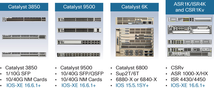
Figure 19-18 outlines some of the platforms that, as of this writing, operate as border nodes within the fabric.
A wide range of fabric border exists, as shown, with a wide range of performance and scalability available. Again, the appropriate choice of fabric border node depends on the scale and functionality requirements involved.
As mentioned previously, a fabric border is implemented either as a dedicated border node or co-located with a fabric control plane function. While some deployments choose the co-located option, others opt for dedicated borders and control planes to provide greater scalability and to lessen the impact of any single device failure within the fabric.
Again, the Catalyst 3850 platforms (fiber based) are typically selected as a border node only for the smallest fabric deployments, or for pilot systems where an SD-Access fabric is first being tested. The amount of memory and CPU horsepower available in the Catalyst 3850, as well as the hardware forwarding performance it offers, may restrict the scalability it offers for this role, however.
Many fabric deployments choose to leverage a Catalyst 9500 switch as a fabric border node. The higher overall performance offered by this platform, both in terms of hardware speeds and feeds and in terms of the multicore Intel CPU used, provides a significant level of performance and scalability for such fabric border use, and makes the Catalyst 9500 an ideal choice for many fabric border deployments.
For branch deployments, the ISR 4000 platforms are also leveraged for this fabric border task, with their CPU and memory footprint making them well suited to this task for a typical branch. The very largest fabric deployments may choose to leverage an ASR 1000 as a fabric border node. This offers the greatest scalability for those SD-Access fabric installations that require this.
When selecting a border platform, please note that not all fabric border functions and capabilities are necessarily available across all of the possible border platforms available.
Please refer to Cisco.com, as well as resources such as the Software-Defined Access Design Guide outlined in the “Further Reading” section at the end of this chapter, for the exact details of the scalability and functionality for each of these fabric border options. The border node scale associated with these platforms varies between platform types, and may also vary between software releases, so referring to the latest online information for these scaling parameters is recommended.
Because new platforms are always being created, and older ones retired, please also be sure to refer to Cisco.com for the latest information on supported devices for the SD-Access fabric border role.
SD-Access Fabric Edge Nodes
Fabric edge nodes serve to attach endpoint devices to the SD-Access fabric. When endpoints attach to the fabric, the edge node serves to authenticate them, either using static authentication (i.e., static mapping of a port to a corresponding VN/SGT assignment) or dynamically using 802.1X and actual user/device identity for assignment to the correct VN/SGT combination, based on that user’s or device’s assigned role.
For traffic ingressing the edge node from attached devices, the fabric edge node looks up the proper location for the destination (RLOC, switch or router) using the fabric control plane node, then encapsulates the ingress packet into VXLAN, inserting the appropriate VN and SGT to allow for proper traffic forwarding and policy enforcement, and subsequently forwards the traffic toward the correct destination RLOC. In LISP nomenclature, the fabric edge node operates as an xTR.
For appropriate QoS handling by the fabric edges as well as intermediate nodes and border nodes, the inner (user) packet DSCP value is copied into the outer IP/UDP-based VXLAN header, and may be used by any QoS policies in use within the fabric network.
Figure 19-19 illustrates the use of fabric edge nodes in SD-Access.
A summary of some of the important functions provided by fabric edge nodes includes
Identifying and authenticating attached wired endpoints
Registering endpoint ID information with fabric control plane nodes
Providing anycast Layer 3 gateway services for attached endpoints
Onboarding users and devices into the SD-Access fabric
Forming VXLAN tunnels with attached APs
As noted, the fabric edge node provides authentication services (leveraging the AAA server provided in the network, such as ISE) for wired endpoints (wireless endpoints are authenticated using the fabric-enabled WLC). The fabric edge also forms VXLAN tunnels with fabric-enabled access points. The details of wireless operation with SD-Access are covered later in this chapter.
A critical service offered by the fabric edge node is the distributed anycast Layer 3 gateway functionality. This effectively offers the same IP address and virtual MAC address for the default gateway for any IP host pool located on any fabric edge, from anywhere in the fabric site. This capability is key for enabling mobility for endpoints within the SD-Access fabric, and is illustrated in Figure 19-20.
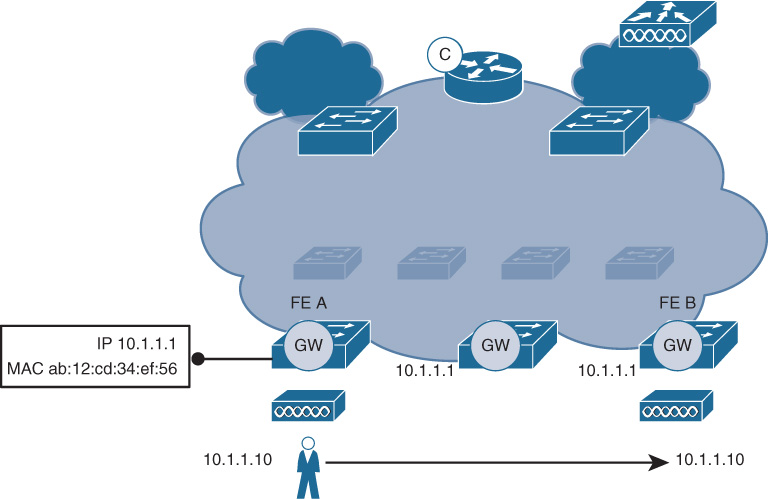
The following are important items of note for the distributed anycast default gateway functionality provided by SD-Access:
It is similar principle to what is provided by HSRP/VRRP in a traditional network deployment (i.e., virtual IP gateway).
The same Switch Virtual Interface (SVI) is present on every fabric edge for a given host pool, with the same virtual IP and virtual MAC address.
If a host moves from one fabric edge to another, it does not need to change its Layer 3 default gateway information (because the same virtual IP/MAC address for the device’s default gateway is valid throughput the fabric site).
This anycast gateway capability is also critical for enabling the overall simplicity that an SD-Access-based deployment offers because it supports the “stretched subnet” capability inherent in SD-Access, as outlined previously in this chapter. This in turn allows enterprises, as noted previously, to vastly simplify their IP addressing planning and deployment.
Organizations deploying SD-Access now reap many of the benefits long enjoyed with wireless overlays for IP addressing—smaller numbers of larger subnets, and more efficient use of IP address space—for both their wired and wireless endpoints attached to their fabric edge switches.
SD-Access Edge Nodes: Supported Devices
Multiple devices can fulfill the task of operating as a fabric edge node. The selection of the appropriate fabric edge node is typically driven by the port densities, uplink speeds, port types (10/100/1000, mGig, PoE or non-PoE, etc.) and edge functionality required.
Figure 19-21 provides an overview of some of the platforms that may be employed in the fabric edge role.
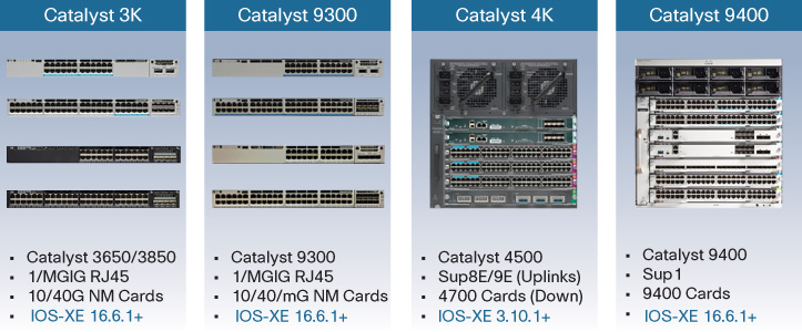
A very important aspect to note with the fabric edge node support in SD-Access is the inclusion of both the Catalyst 3850 and 3650 platforms. This capability to support the fabric edge capability on these platforms is a direct result of the outstanding capability provided by the flexible, programmable Unified Access Data Plane (UADP) chipset they employ.
Every Catalyst 3850 and 3650 ever produced, since the introduction of the platform, can (with the appropriate software load and licensing) be provisioned into an SD-Access fabric and operate as a fabric edge node. As one of the leading access switch platforms in the industry, deployed by many thousands of Cisco customers worldwide, this opens up the ability to deploy VXLAN-based SD-Access fabrics to many networks that would otherwise have to wait for a multiyear hardware refresh cycle before the migration to a next-generation network design could be considered.
The ability to leverage these widely deployed enterprise switches as fabric edge nodes in SD-Access is a direct result of Cisco’s inclusion of programmable ASIC hardware into these platforms. This provides an outstanding level of investment protection for Cisco customers using these platforms, and highlights the importance of the flexible, programmable UADP ASIC that was examined in detail in Chapter 7.
In addition, the Catalyst 4500 using Supervisor 8/9 (for uplinks to the rest of the fabric network) and 4700-series linecards (for downlinks to attached devices) can be employed as an SD-Access fabric edge switch, thus providing outstanding investment protection for those sites that prefer a modular access switch architecture.
Please refer to Cisco.com, as well as resources such as the “Software-Defined Access Design Guide” outlined in the “Further Reading” section at the end of this chapter, for the exact details of the scalability and functionality for each of these fabric edge options as shown. The fabric edge scale associated with these platforms varies between platform types, and may also vary between software releases, so referring to the latest online information for these scaling parameters is recommended.
Because new platforms are always being created, and older ones retired, please also be sure to refer to Cisco.com for the latest information on supported devices for the SD-Access fabric edge role.
SD-Access Extended Nodes
In some types of deployments, it might be desirable to connect certain types of network devices below the fabric edge. These may be devices that are specific types of Layer 2 switches, such as switches that provide form factors other than those supported by the fabric edge node, or that are designed to work in environments too hostile or demanding for a standard fabric edge node to tolerate.
In an SD-Access deployment, such devices are known as extended nodes. These plug into a fabric edge node port and are designated by Cisco DNA Center as extended nodes. Operating at Layer 2, these devices serve to aggregate endpoints attached to them into the upstream fabric edge node, at which point the traffic from these extended nodes is mapped from their respective Layer 2 VLANs into any associated VNs and SGTs, and forwarded within the SD-Access fabric. For this purpose, an extended node has an 802.1Q trunk provisioned from the fabric edge node to the attached extended node.
Because extended nodes lack all the capabilities of a fabric edge node, they depend on the fabric edge for policy enforcement, traffic encapsulation and decapsulation, and endpoint registration into the fabric control plane.
Supported extended nodes for an SD-Access fabric deployment as of this writing include the Catalyst 3560-CX compact switches, as well as selected Cisco Industrial Ethernet switches. Only these specific types of switches are supported as extended nodes, as they are provisioned and supported by Cisco DNA Center as an automated part of the SD-Access solution overall.
The ability to “extend” the edge of the SD-Access fabric using these switches allows SD-Access to support a broader range of deployment options, which traditional Cisco edge switches might not otherwise be able to handle alone. These include such diverse deployment types as hotel rooms, cruise ships, casinos, factory floors, and manufacturing sites, among others.
Please refer to Cisco.com, as well as resources such as the Software-Defined Access Design Guide outlined in the “Further Reading” section at the end of this chapter, for the exact details of the scalability and functionality for each of these fabric extended node options. The extended node scale associated with these platforms varies between platform types, and may also vary between software releases, so referring to the latest online information for these functionality and scaling parameters is recommended.
Because new platforms are always being created, and older ones retired, please also be sure to refer to Cisco.com for the latest information on supported devices for the SD-Access fabric extended node role.
Now that we’ve examined the options available for the SD-Access fabric wired infrastructure, let’s move on to examine wireless integration in an SD-Access fabric deployment.
SD-Access Wireless Integration
Wireless mobility is a fact of life—and a necessity—for almost any modern organization. Almost all devices used in an enterprise network offer an option for 802.11 wireless connectivity—and some devices, such as smartphones and tablets, are wireless-only, offering no options for wired attachment. Today’s highly mobile workforce demands secure, speedy, reliable, and easy-to-use access to wireless connectivity.
SD-Access offers a sophisticated new mode for wireless deployment, allowing for direct integration of wireless capabilities into an SD-Access fabric, and allowing wireless endpoints and users to access all of the benefits that a fabric deployment provides—including macro- and micro-segmentation, group-based policy enforcement, and stretched subnets, as well as full distributed traffic forwarding.
Segmentation, group-based policies, and stretched subnets were examined earlier in this chapter, and elsewhere in this book, in some detail, including their benefits, so in this section we’ll focus on the distributed traffic forwarding that fabric offers and see how this provides significant benefits for wireless deployments.
One significant trend in 802.11 wireless over recent years has been the move to ever-greater speeds offered by APs for endpoint attachment over RF. From the early days of 11-Mbps 802.11b, to 54 Mbps with 802.11a/g, it is now common to see enterprises deploying 802.11ac Wave 1 and Wave 2 APs that offer well over 1 Gbps of real-world wireless bandwidth to endpoints and users. In the future, the new 802.11ax standard will push this limit closer to 10 Gbps, while at the same time increasing the efficiency of usage of the wireless medium.
Figure 19-22 depicts the evolution of wireless from a “nice-to-have” capability to its present, and future, status as a mission-critical capability for many organizations worldwide.
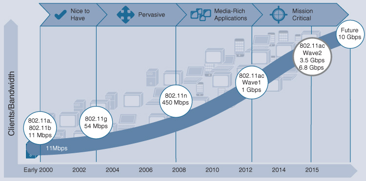
As wireless bandwidths increased, they placed ever-greater pressures on the traditional centralized method of wireless LAN deployment. Many organizations deploy centralized wireless, in which APs form Control and Provisioning of Wireless Access Points (CAPWAP) tunnels back to a central WLC, or cluster of WLCs, and forward all wireless client data, as well as control plane traffic, over these CAPWAP tunnels.
This method of wireless deployment (known as Cisco Unified Wireless Network, or CUWN) has several important benefits, including simplified deployment and operation (because all IP addressing and policy enforcement is handled at the WLC) and integrated secure guest access. Some of these benefits are outlined in Figure 19-23.
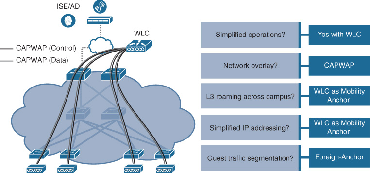
However, this method of traditional centralized wireless deployment lacks some of the strengths that typically accrue to a Cisco wired network deployment, including support for segmentation, greater scalability and capability for complex policies for QoS and security, and the scalability that comes with a fully distributed forwarding and feature plane.
Some of these benefits for a traditional wired network are outlined in Figure 19-24.
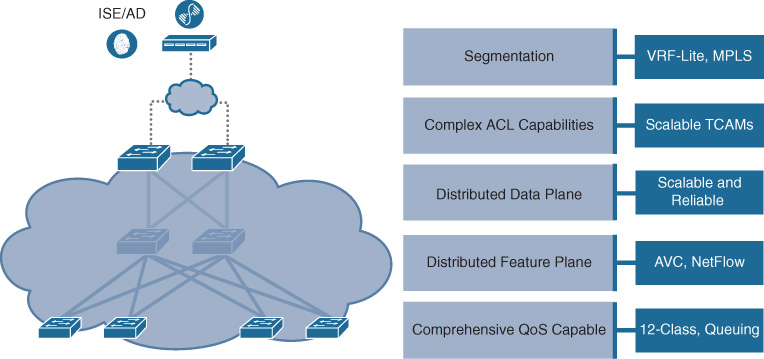
An SD-Access wireless deployment provides the best of both of these worlds, offering:
The simplicity of a traditional centralized wireless deployment (retained by using the WLC as the primary point for wireless control)
The scalability of a traditional wired deployment (by employing a fully distributed data plane, leveraging the switched network infrastructure for traffic forwarding).
The feature richness of a traditional wired deployment (by providing integrated functionality for secure segmentation and policy enforcement)
Let’s examine how SD-Access wireless integration works, to see these capabilities in action.
SD-Access Simplified Wireless Control Plane
SD-Access wireless retains and builds upon the traditional simplicity of wireless deployments, by continuing to leverage the feature-rich Wireless LAN Controller (WLC) as the central point for wireless AP deployment and RF management. In an SD-Access fabric, the WLC continues to be used to onboard clients, manage APs, and control the RF domain, retaining the simplicity and operational paradigm that wireless network managers have become accustomed to over many years.
However, the fabric-enabled WLC is integrated with the SD-Access fabric control plane, such that when a wireless client attaches or roams, an update is always sent to the fabric control plane node, noting which switch (RLOC) the wireless client is located behind (based on which AP it is associated with). This ensures that, in a fabric deployment, the SD-Access control plane node always serves as a single point of reference for where any endpoint is located in the fabric network—wired or wireless.
Figure 19-25 illustrates the basic functions performed by a WLC that is integrated into an SD-Access fabric.
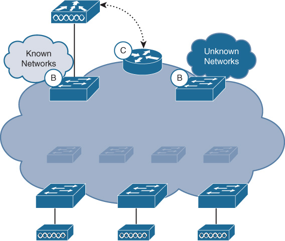
There are several important items to note concerning the operation of a WLC within a fabric-enabled wireless system:
The fabric-enabled WLC connects outside of the fabric, accessing the SD-Access fabric via the fabric border, in the underlay network.
The fabric-enabled WLC registers wireless clients with the fabric control plane (indicating which RLOC [fabric edge switch] they are attached to).
Fabric-enabled APs are provisioned in a dedicated IP host pool within the fabric (in the VXLAN overlay).
SSIDs (to which wireless clients attach) use regular IP host pools for traffic forwarding and policy application.
With the use of a fabric-integrated WLC, any endpoint within the SD-Access fabric domain can query the fabric control plane for any endpoint—wired or wireless—and always forward traffic within the fabric overlay to the correct destination, thus enabling seamless connectivity across the fabric to and from any endpoint.
The integration between the WLC and the fabric control plane node is illustrated Figure 19-26.
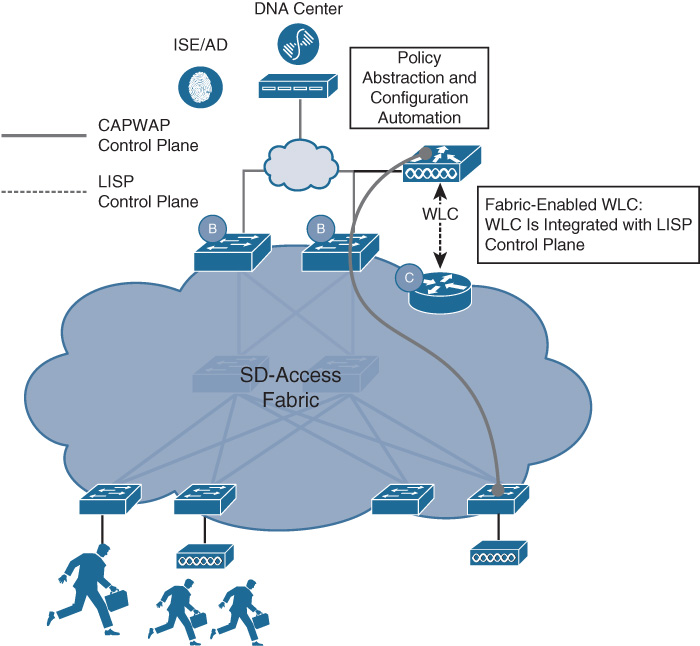
There are several important items to note concerning the control plane integration of wireless with the SD-Access fabric:
Automation: Cisco DNA center simplifies the overall fabric deployment, including the wireless integration components.
Centralized wireless control plane: The WLC still continues to provide wireless client session management, AP management, Radio Resource Management (RRM), and overall mobility functions.
Integration with the LISP control plane: Operating with AireOS 8.5 or above, the fabric-enabled WLC integrates with the LISP control plane to provide updates to the LISP control plane nodes for wireless clients as they attach and roam. Thanks to this integration, wireless mobility is incorporated into the fabric deployment.
Each fabric-enabled access point retains a control plane CAPWAP tunnel back to its associated WLC for management. This retains the simplicity of management and operation that wireless operators are accustomed to and eases the migration path toward a fabric-integrated wireless deployment.
However, unlike in a traditional CUWN deployment, this CAPWAP tunnel is not used for data plane forwarding—it is purely a control plane tunnel only between the AP and WLC. In SD-Access, the wireless data plane is entirely distributed, as outlined in the following section.
A more detailed review of the integration between the fabric-enabled WLC and the SD-Access fabric control plane is provided in Figure 19-27.
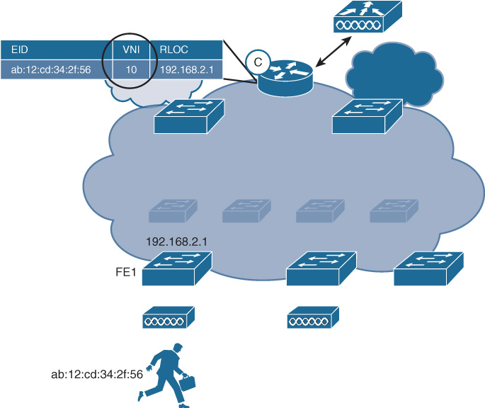
There are several important items to note concerning wireless integration with the SD-Access fabric. First, for wireless clients, the client’s MAC address is tracked and is used as the EID. Second, because wireless roams are handled as Layer 2 roams within the fabric—enhancing deployment efficiency—a Layer 2 VNI is employed within the fabric for this use. And finally, it is necessary that the WLC and the APs be co-located at the same site (i.e., not separated over a WAN), due to the tight timing constraints driven by the integration of the WLC with the fabric control plane.
Overall, the method used for integrating wireless with SD-Access fabric retains the traditional simplicity of the wireless control plane, while ensuring seamless operation in a fabric deployment model.
Now, let’s move on to examining how SD-Access wireless provides data plane integration, and the benefits this provides.
SD-Access Optimized Wireless Data Plane
SD-Access wireless helps to address the ever-increasing needs for both bandwidth and sophisticated services for wireless traffic by leveraging a fully distributed data plane approach. With the move to 802.11ac Wave 2 and, in future, 802.11ax, the necessity for a distributed data plane forwarding option for wireless traffic becomes ever more apparent.
With SD-Access wireless, each fabric-enabled AP, in addition to the CAPWAP control plane tunnel it uses to the fabric-enabled WLC, forms a VXLAN data plane tunnel to its adjacent fabric edge switch, and uses this VXLAN tunnel for forwarding of all endpoint data plane traffic. This is illustrated in Figure 19-28.
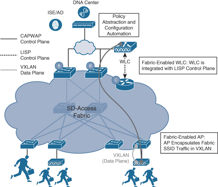
Important items to note here include the following:
Optimized distributed data plane: By leveraging the fabric overlay with its distributed anycast default gateway and associated stretched subnet functionality, the ability to provide a single IP subnet for all attached wireless devices for a given SSID is provided, without complications. All roams within the fabric-enabled wireless deployment are handed as Layer 2 roams.
VXLAN from the AP: Allows hierarchical user/device policy and segmentation capabilities (based on VN/SGT groupings) to be provided for wireless clients, in exactly the same manner as wired clients, right from the AP—thus allowing for a truly unified enterprise access policy.
The use of VXLAN for the data plane tunnel between the AP and its adjacent fabric edge switch ensures that all of the VN and SGT information associated with the wireless clients is passed to this adjacent wired switch and used for policy enforcement.
At the same time, the use of a one-hop VXLAN tunnel ensures that the adjacent switch is always seen by the SD-Access fabric control plane as the RLOC for other devices to forward traffic to within the fabric, avoiding an “RLOC explosion” that might otherwise accrue if the fabric control plane had to track every fabric-enabled AP directly.
By decapsulating, inspecting, and then re-encapsulating all wireless traffic within the fabric at the wired access switch, the scalability and feature set of the switched infrastructure is leveraged to the greatest extent possible, while still retaining seamless mobility and ease of operation, deployment, and use. And thanks to the performance offered by the flexible, programmable UADP ASIC, with its high-speed recirculation functionality optimized for tunneling (as examined in Chapter 7), this capability is offered with very high throughput.
A further depiction of the integration between the fabric-enabled AP and its adjacent fabric edge switch is illustrated in Figure 19-29.
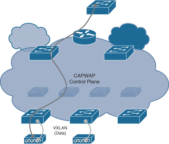
A few items of note here are that the AP operates in Local mode and is directly adjacent to the fabric edge switch. (APs can also be attached to an extended node switch, if these are in use.) Also, APs apply policies such as Cisco Application Visibility and Control (AVC) and QoS locally on the AP itself to distribute these functions as far as possible toward the network edge and thus further increase scalability.
SD-Access Over-the-Top (OTT) Wireless Support
For completeness, it should be noted that that wireless deployments in SD-Access can also be accommodated in an Over-the-Top (OTT) deployment mode, in which the existing CAPWAP tunnels (for both data plane and control plane) are retained from the APs to the WLCs, just as they are today—using the SD-Access fabric only for transport (i.e., not integrated directly as with fabric-enabled wireless).
This capability for OTT wireless use is valuable as a stepping-stone to an SD-Access deployment, especially in cases where the existing deployed wireless network equipment does not support the use of fabric-enabled wireless operation, or in the event that the organization involved simply wishes to deploy a more traditional wireless environment while upgrading its wired deployment to SD-Access.
Also note that OTT wireless does not provide all of the benefits of a fabric-integrated SD-Access wireless deployment. A truly integrated SD-Access wireless deployment provides support for integrated two-level segmentation (macro and micro, based on VN and SGT), greater scalability via the use of a distributed data plane, and consistent policy for both wired and wireless users. Although an OTT wireless deployment lacks these capabilities, it remains an option in the event that a fabric-integrated wireless deployment cannot be undertaken for any reason.
SD-Access Wireless: Supported Devices
Multiple devices are used within a fabric-enabled wireless deployment, including many existing WLCs as well as 802.11ac Wave 2 and (with certain caveats) 802.11ac Wave 1 APs.
Figure 19-30 provides an overview of some of the platforms that are employed in an SD-Access fabric-enabled wireless deployment.
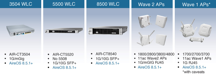
The ability to reuse the existing WLCs and APs, as shown, in a fabric-enabled wireless deployment assists in easing the migration to SD-Access, and provides a significant level of investment protection for existing Cisco wireless deployments.
Please refer to Cisco.com, as well as some of the references noted at the end of this chapter, for the exact details of the scalability and functionality for each of these wireless options as shown, as well as for the caveats associated with the use of 802.11ac Wave 1 APs in a fabric deployment.
The scale associated with these various wireless platforms varies between platform types, and may also vary between software releases, so referring to the latest online information for these scaling parameters is recommended.
Because new platforms are always being created, and older ones retired, please also be sure to refer to Cisco.com for the latest information on supported devices for SD-Access wireless capability.
The benefits that accrue to an integrated wireless deployment with SD-Access—seamless and simple control plane integration, the use of a distributed data plane, and the ability to leverage the strengths of SD-Access for segmentation and security in a common way for both wired and wireless users—all serve to assist in driving wireless networking toward a more-scalable and feature-rich future, a future that offers consistent and powerful capabilities for wired and wireless users alike.
SD-Access Multicast Support
Finally, an important aspect of many enterprise network deployments is the use of IP multicast. Multicast is supported in an SD-Access fabric deployment. The method of multicast replication used is known as “head-end” replication, meaning that multicast traffic ingressing an SD-Access fabric node (edge or border) will be replicated by that device into multiple unicast VXLAN-encapsulated copies of the original (inner) multicast packet, with one copy sent to each RLOC that is receiving the multicast stream. Once these unicast VXLAN-encapsulated copies reach each destination RLOC, they are then decapsulated (revealing the inner, original IP multicast packet), which is then locally replicated by that RLOC to any attached multicast receivers.
This method of multicast forwarding and replication thus provides end-to-end multicast capability across the SD-Access fabric, in a simple and straightforward fashion. This method also has the benefit of not requiring the underlay network to be multicast-enabled, in order to support IP multicast capability in the overlay fabric.
A future version of SD-Access is planned to provide “native” IP multicast replication, meaning that rather than having the head-end (ingress) RLOC replicate out multiple unicast-encapsulated copies of the multicast traffic, an underlay multicast group will be used to provide the replication capability between the RLOCs involved. This has the benefit of distributing the multicast replication load across the underlay network and its many devices, at the cost of having to configure IP multicast support in the underlay network. However, because configurations are automated within Cisco DNA Center, this should impose little extra burden on the network administrator once available.
SD-Access Case Study
Now that we have examined all the basics of Software-Defined Access, let’s delve into a case study and examine how to use Cisco DNA Center to define, deploy, and manage the various components that make up an SD-Access fabric.
Let’s start in Cisco DNA Center. As detailed in other chapters of this book, Cisco DNA Center offers a next-generation solution for network definition, deployment, and ongoing maintenance and operation. As noted previously, when you first log into Cisco DNA Center, you are offered a four-step workflow—namely, Design, Policy, Provision, and Assurance. Let’s start this journey into the SD-Access case study with Design, where you provide all the basic information that is necessary as you begin to build out your fabric solution.
Please note that this is necessarily an abbreviated description of building out and operating an SD-Access fabric with Cisco DNA Center, due to space limitations inherent with a single chapter within this larger volume. More complete and detailed explanations of building out an SD-Access fabric are contained within the “Further Reading” references at the end of this chapter. However, this case study provides a good overview of the major steps involved and serves to illustrate how simple, powerful, and flexible Cisco DNA Center makes building out an entire fabric-based network solution.
With that said, let’s get started!
In the Cisco DNA Center GUI, click Design to access the Network Hierarchy screen displayed in Figure 19-31. This shows an overall map, indicating the various positions where sites were already defined, and where new sites can be defined prior to deployment. In this example, we are reviewing an educational system with sites scattered across various locations in the United States.
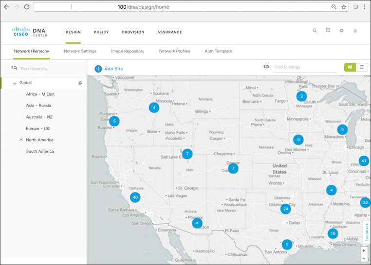
As you can see, the previously defined sites are located across the United States. The bubbles indicate the number of sites within each region, and by mousing over an area and clicking it, a zoomed-in view is obtained, all the way down to the individual site level. Sites are also organized into a hierarchy, as you can see on the left side, allowing for easy access to the various defined sites. A new site is added simply by clicking the blue plus sign icon next to the Add Site text—a common paradigm within Cisco DNA Center. Sites contain one or multiple buildings, each of which contains floors complete with floor maps and layouts.
In this case, let’s zoom into an already-defined site in San Jose and start examining the network definition for the site.
Figure 19-32 shows some of the basic network definitions for the site, noting the common deployment items for the site including DNS servers, DHCP servers, syslog servers, and the like.
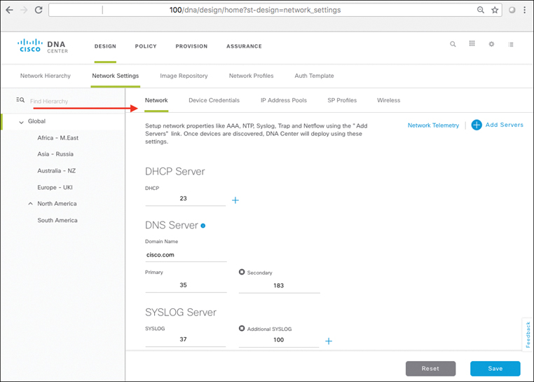
Note
IP addresses in the figures have their leading octets deliberately obscured to ensure the security of the site involved.
Note that many network settings can be defined at a higher site hierarchy level and then inherited to sites below that in the hierarchy. In fact, what you are viewing in Figure 19-32 is the Global settings for the items noted, which a lower-level site such as the San Jose site could inherit, or override with more site-specific settings if and as needed. This ability to provide higher-level inheritance with site-specific override capability makes defining new sites within Cisco DNA Center very easy.
In addition to the settings shown in Figure 19-32, additional elements that can be defined for the network settings for a site include definitions for the AAA servers in use, the SNMP servers in use, the NetFlow collectors server to use, and the NTP server in use, as well the local time zone and message of the day for the site.
Additional important elements of defining a site are the IP host pools (subnets) which are defined for, and made available, at the site. These are the IP subnets provided for use by users, devices, and things at the sites involved. Figure 19-33 illustrates how an IP address pool is defined for the site involved; observe in the background that several other IP address pools already have been defined. Note that to get to this screen we navigated to Design > Network Settings and clicked Edit next to an existing IP host pool.
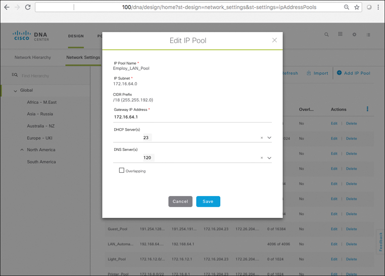
For each IP host pool, a subnet range is defined, complete with the assignment of a gateway IP address (which is used as the distributed anycast default gateway for the subnet). DHCP and DNS servers are also assigned from those previously defined in the Network Settings area.
With the critical servers and services assigned for a site, it is now timely to review the status of the various devices that may end up being used for establishing the fabric at the site involved, as shown in Figure 19-34. These devices are discovered by Cisco DNA Center by pointing at a given “seed device” to which Cisco DNA Center has connectivity. Cisco DNA Center then logs into that device (using credentials supplied by the network administrator) and proceeds to “walk” across the network, discovering devices, adding them into the Cisco DNA Center inventory, and noting the network topology interconnecting them.
As you see, devices so discovered and added into the inventory are analyzed and shown with their software versions, device types, and revisions noted for easy review. Any software images standardized on by the organization can be denoted as “golden” images, making it simpler to determine at a glance whether devices are in compliance with organizational standards for software deployment. Note that the arrow as shown is not part of the Cisco DNA Center GUI; instead, we are using it simply as an aid to where to look on the screen.
Cisco DNA Center also provides a tool that can be used to automate the deployment of the network itself—namely, LAN Automation. This capability again employs a seed device, and starting from that device can “walk out” up to two layers within the network hierarchy and automate the deployment of new devices it so discovers. This automation includes, and is intended to support, the deployment of an automated underlay suitable for the later overlay of an SD-Access fabric.
If deployed with LAN Automation, this underlay is built using the routed access deployment model (i.e., routing all the way down to the access layer), using Intermediate System to Intermediate System (IS-IS) as the routing protocol. Alternatively, if the network already exists, or the organization prefers to deploy its own underlay with its own chosen IGP routing protocol, this can also be accommodated. Further details are available in some of the items noted for “Further Reading” at the end of this chapter, such as the “SD-Access Design Guide” noted.
Now that you have seen how to define all the basics for your network access—your site hierarchy and sites, critical services, IP subnets, and devices—let’s begin to delve into the design of various network policies within the Policy workflow in Cisco DNA Center. This is illustrated in Figurer 19-35.
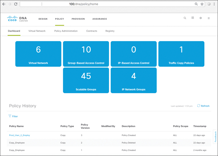
Initially, you land on a dashboard for the Policy workflow in Cisco DNA Center, showing an overview of the various polices already defined. This example already has a total of 6 virtual networks defined, a total of 10 group-based access control policies (leveraging SGACLs), and a total of 45 Scalable Groups (using SGTs), along with various other network policies for IP-based groupings and traffic copy policies.
You can also see a summary of the history of the policies that were created or modified in Cisco DNA Center, including the type of policy, the version and scope, a description of what action was taken with regard to each policy, and the time that this action took place. This is very valuable for keeping track of which policies were created or modified, when, and by whom.
First, let’s zoom over into the Virtual Network area and see what is defined for VNs currently, as shown in Figure 19-36.
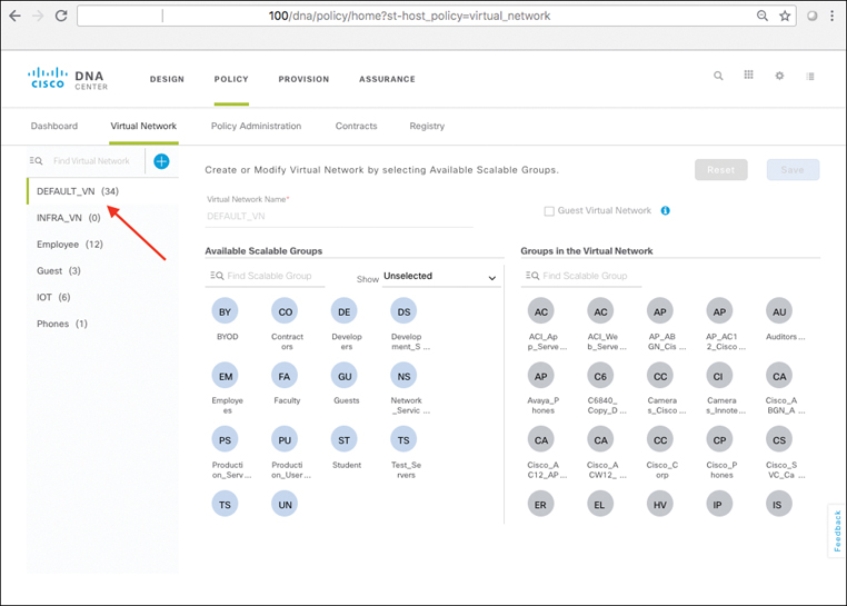
Here, you see on the left side of the screen all six of the VNs currently defined. Initially, as indicated by the arrow, you are viewing the Default VN (DEFAULT_VN). This VN always exists in a fabric, and is the VN into which users, devices, and things are mapped by default if no other VN is chosen. The groups shown on the far right side are already mapped into this VN, meaning that any user or device that attaches and is assigned to one of these groups is mapped into the Default VN. The groups shown on the left side are available to assign into this VN if desired. This is done merely by dragging and dropping these groups into the right-side pane and clicking Save.
Now, you may ask yourself, where do all of these groups come from? Most commonly, the groups are created within Cisco ISE and then imported into Cisco DNA Center when ISE is integrated with Cisco DNA Center as its assigned AAA server. In turn, ISE may have obtained these groups from an outside source such as Active Directory (assuming the organization involved has ISE and AD integration configured).
Another VN that you can observe in the list is the INFRA_VN. This is a VN that “infrastructure” devices such as access points and extended nodes are mapped into. This VN is somewhat “special” in that users are never mapped into this VN—it is reserved for infrastructure devices only. The INFRA_VN is also special in that it is not mapped into a VRF instance like other VNs are—it is mapped into the Global Routing Table (GRT) in the underlay, but with a LISP instance in the GRT (i.e., VRF 0) to keep track of these infrastructure devices and their locations. This provides maximum simplicity of operation for these devices, as such devices (for example, APs) often need to contact their related services (such as a WLC, for example) located outside of the fabric, and locating these devices in the underlay GRT allows for simplified configuration at the fabric border to facilitate such connectivity.
The other VNs in the list (Employee, Guest, IOT, and Phones) were created by the network manager. In this example, these are the VNs associated with a university deployment. Each of these VNs is mapped into a corresponding VRF in the fabric overlay.
Creating a new VN is very simple. Simply click the blue plus sign icon, as shown in Figure 19-37.
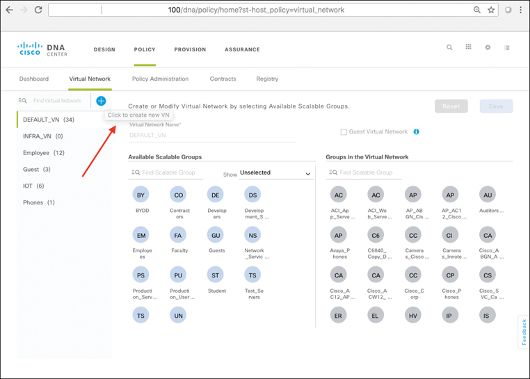
After selecting to add a new VN, simply type in the new name and click Save. This triggers Cisco DNA Center to provision the VN into all of the associated devices within the fabric, creating all of the VRFs, Route Distinguishers, Route Targets, and other ancillary components necessary to set up the VN for operation.
Figure 19-38 shows how to set up a new VN called Cameras, into which you could place IP-based security cameras. After setting up the new VN, you can assign groups into it simply by dragging and dropping them, as shown on the right in Figure 19-38.
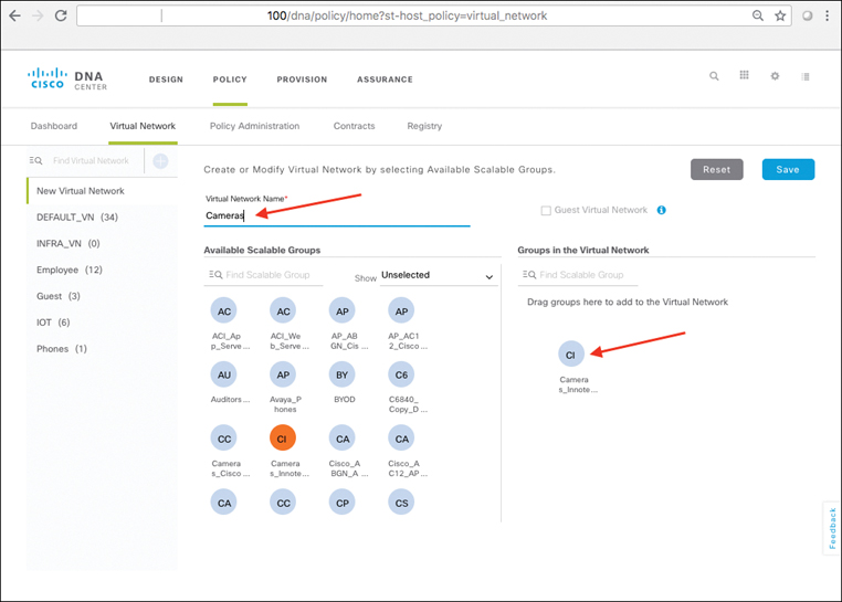
In this case study, the IP-based cameras were not yet unboxed and ready to plug into the network, so the configuration was not saved. It’s important to note that none of the changes you make in Cisco DNA Center are deployed until you click Save, thus providing ample opportunity to explore the interface without actually making any network changes.
Now that you have explored VNs, click the Policy Administration tab to see how to work with groups and group-based policies in Cisco DNA Center. Figure 19-39 shows a quick summary of all the various group-based policies that are currently defined for the fabric infrastructure in the example.
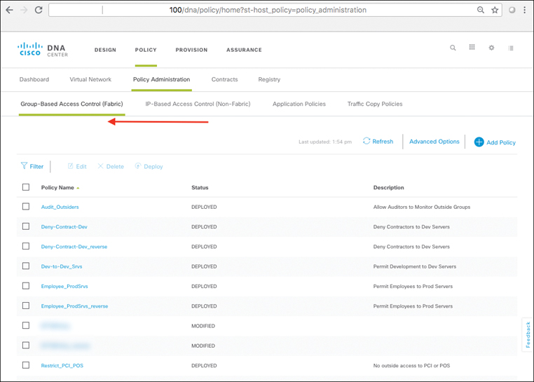
From here, you see all the policies that currently exist. Let’s explore the one named Employee_ProdSrvs. Clicking its name opens the Details dialog box shown in Figure 19-40. This policy is intended to provide employees with access to production servers and services via the fabric.
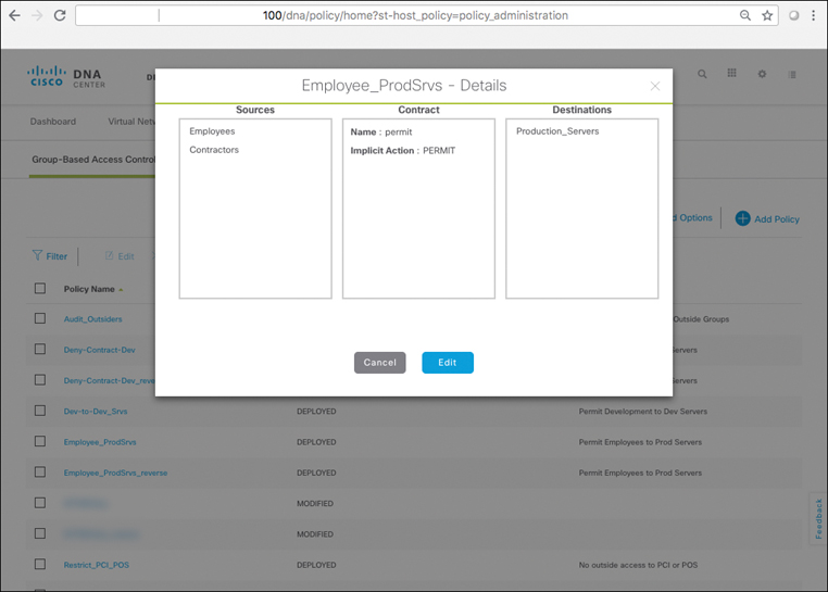
Here, you can observe that the policy is defined to allow two groups, Employees and Contractors, access to (permit) any server or service in the group Production_Servers. Any user or device authenticating into either of these source groups is allowed access to any server or service mapped into this destination group, based on this policy as shown.
At this point, you are just viewing the policy. Figure 19-41 shows what happens if you click the Edit button for this policy.
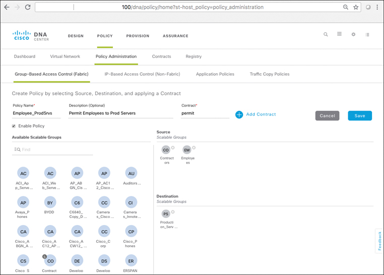
Creating or editing a policy basically consists of three steps: defining the source group(s), defining the destination group(s), and creating a contract between them that specifies how the groups involved can interact, or the action to be taken on their traffic flows. Here, you see all the components defined that allow for the desired policy involved in this example—namely, a source of Employees or Contractors, a destination of Production_Servers, and an action of Permit.
Let’s say a request had just come through to allow an Auditors groups within the university access to these same servers and services. Figure 19-42 shows how to accommodate this request.
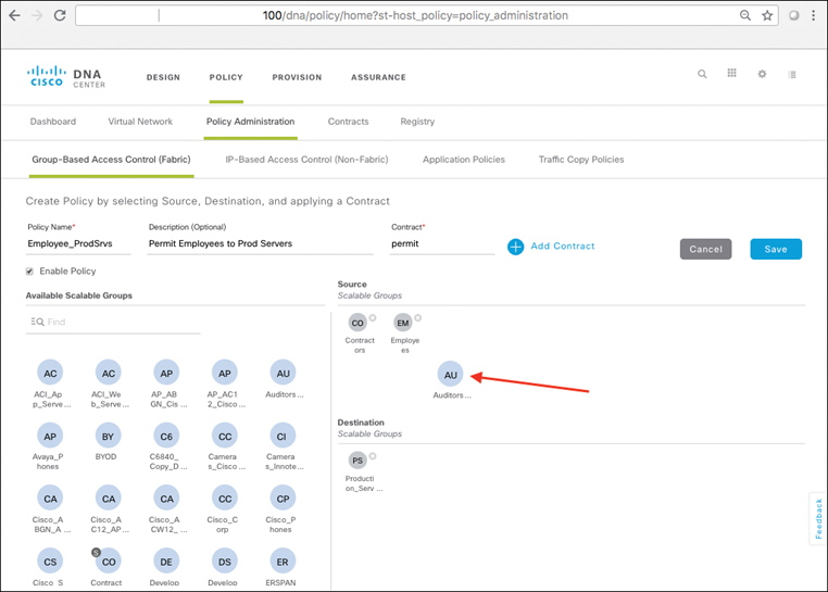
Here, you would simply drag the assigned group (Auditors) into the source area for Scalable Groups assigned to the policy. And that’s it! It’s really that simple. But remember, nothing is committed until you click Save. Figure 19-43 shows the policy being saved.
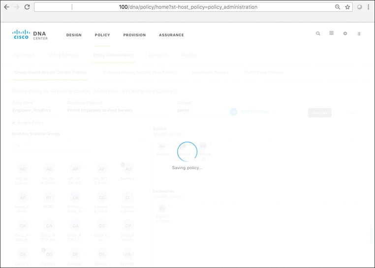
Cisco DNA Center sanity-checks the policy and, once done, creates the necessary policy configurations and pushes the policy so created over to ISE. ISE in turn deploys the updated group-based policy to all the appropriate devices within the fabric. All of this happens seamlessly and without further need for intervention by the network operator.
To provide a positive indication that these changes took place, the pop-up message shown in Figure 19-44 briefly appears within Cisco DNA Center to indicate the success of the policy change.
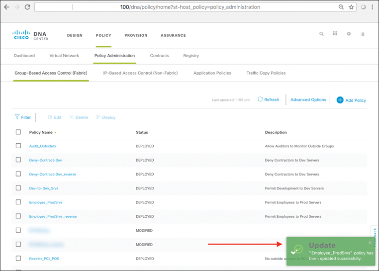
Now that we have explored policy configuration and alteration, let’s delve into provisioning the fabric itself. Switching to the Provision workflow in Cisco DNA Center again presents the Device Inventory, as shown in Figure 19-45.
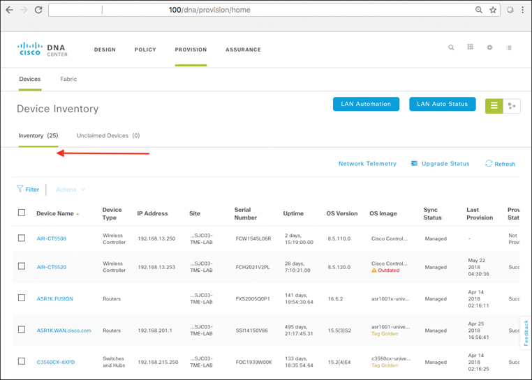
On the Inventory tab, you can assign to sites the devices that you discovered and added to your inventory, and you can provision them to prepare them for the various roles that they will take on within the fabric. Again, you can review OS images, check the provisioning status, and check the sync status (indicating whether Cisco DNA Center has obtained the necessary copy of the device’s configuration).
Since you are interested in building out a fabric, click the Fabric tab. This brings you to a screen such as the one illustrated in Figure 19-46.
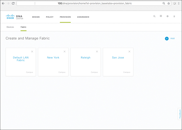
In this screen, you see a summary of all the various fabrics set up so far. In this example there are four: the Default LAN Fabric, along with three others, New York, Raleigh, and San Jose—locations where the university has campuses. Adding a new fabric is as a simple as clicking the blue plus sign icon and assigning the appropriate name and site type. However, in this example, let’s explore an existing fabric and see how to assign new devices to an existing deployment.
Figure 19-47 shows the screen presented after selecting the San Jose fabric.
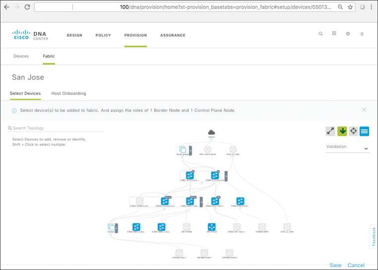
There’s quite a bit going on here, so take your time and explore it. First, notice that you need to assign at least a border node and a control plane node to build out the fabric. The example topology shown actually has four border nodes: two defined on a pair of Catalyst 6800s (a 6807 and a 6880), one defined on a Catalyst 6840, and one defined on a Catalyst 9500. The topology also has a single control plane node, as defined on a second Catalyst 9500. Most networks actually have two control plane nodes deployed for redundancy, but this example is still early in the deployment cycle and so only has one defined. This is shown “zoomed in” in Figure 19-48, for greater clarity. Please note that all devices that are currently added to and participating in the fabric are shown in a blue color (non-fabric or underlay-only devices are shown in gray).
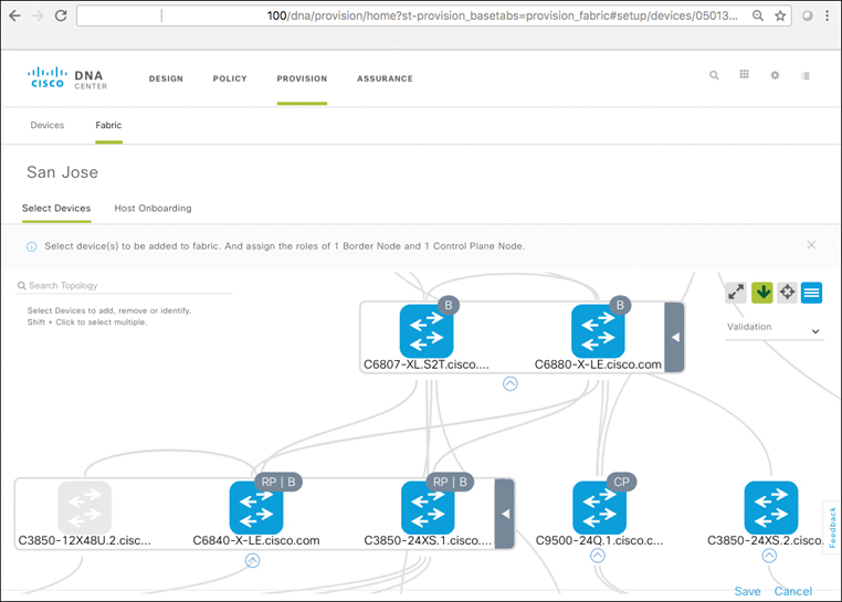
As you can see, border nodes are clearly marked with a “B” and the control plane node is indicated with a “CP.” Again, this example has a total of four borders and only one control plane node, as shown in Figure 19-48.
Another item of note is that two of the nodes acting as borders are also marked with “RP,” indicating these nodes are acting as Rendezvous Points for the multicast deployment within the fabric. As per standard multicast operation, the RPs are where the multicast sources are joined to the appropriate destinations, using Protocol Independent Multicast (PIM) as the control plane for operation of the multicast system.
It is worth noting that the default mode of operation for multicast within the fabric environment is via head-end replication—meaning that all multicast packets for the overlay network are replicated at the ingress node (typically, an edge switch) and sent as individual unicast-VXLAN-encapsulated packets to each egress switch, which then decapsulates the unicast VXLAN outer header, exposing the inner user multicast packet, which then undergoes local multicast replication for delivery to any receivers for that multicast group at the egress node.
Although this mode of operation is not as efficient as true underlay multicast replication is, it does have the beneficial property of not requiring the underlay network itself to be multicast-enabled—a very important consideration for many existing enterprise networks that may desire to have multicast available for use by fabric-based overlay applications but never have gone to the time and effort of enabling multicast network-wide on their existing (underlay) network infrastructures. If multicast is in fact available in the underlay, a future revision to the SD-Access solution is currently planned to enable the underlay multicast system to be leveraged for distributed multicast replication.
The San Jose fabric also has a number of edge switches defined, based on Catalyst 3650s and other switches, as shown in Figure 19-49.
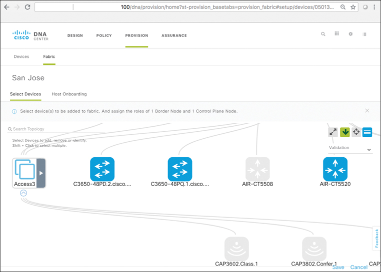
Notice the close-up view of the various edge switches added to the fabric, along with wireless devices (APs and WLCs). As shown, San Jose already has two Catalyst 3650s added to the fabric, along with a WLC 5520 and a number of APs (note, the 3602 AP shown is not fabric-capable, but the 3802 AP is). You know that these are fabric edge switches because they are shown in a blue color (thus added to fabric), but they do not have any tag on them as the border or control plane switches have. Any devices so colored but untagged are edge switches as shown in the topology.
One interesting item also shown here is the access grouping called Access3. For additional clarity, Cisco DNA Center allows devices shown in the topology view to be collapsed together for simplified viewing. In this case, clicking the triangle symbol expands this device group, as shown in Figure 19-50.
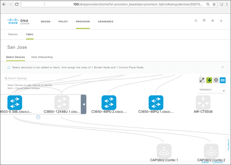
Figure 19-50 reveals that this device group contains a Catalyst 4503 edge switch already added to the fabric, along with a Catalyst 3850 switch that has not been added.
Let’s see how to add a switch into the fabric. The result of selecting a Catalyst 9300 24-port switch, clicking it in the topology, and selecting Add to Fabric is illustrated in Figure 19-51.
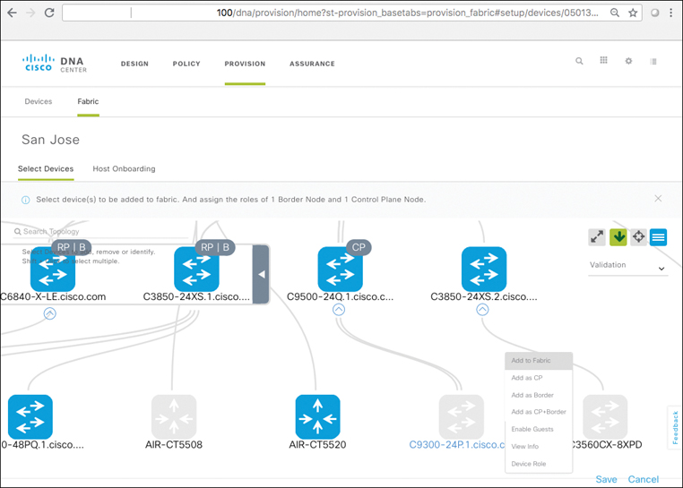
Because the device is not being added as a border or control plane, it is by default added as an edge switch. Right-clicking the name of the device and choosing Add to Fabric (and zooming back out a bit for clarity on the entire topology) opens a screen similar to that shown in Figure 19-52.
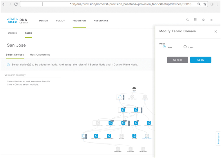
Because converting a switch to be a fabric edge involves fairly substantial changes to the switch’s configuration—adding a LISP instance, configuring VRFs and new IP subnets, pointing it to the fabric’s control planes and default border elements, and much more—the choice is given to deploy this configuration immediately or defer it to a later (scheduled) time. In this case study, the switch was deployed immediately, launching the update screen shown in Figure 19-53.
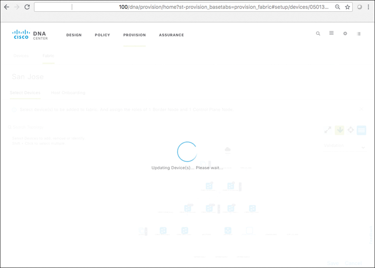
At this point, all the necessary switch configurations are created by Cisco DNA Center, deployed to the switch or switches involved (because many devices can be deployed at once by the network manager), and checked for proper deployment. Once the configuration is verified as correct, the network icon on the map changes from gray to blue. Success! A new edge switch was added to the fabric.
Adding a WLC to the fabric is accomplished in much the same way, with APs continuing to be deployed and managed via the WLC as always—but now operating in a distributed mode using local VXLAN tunnels to drop off user data directly at the edge switch, leveraging the distributed anycast default gateway, stretch subnets, and VN/SGT-based policies for wireless traffic just as is done for wired traffic. In this example, the WLC 5520 and any compatible APs are deployed in a fabric mode of operation.
Finally, let’s take a closer look at assigning IP host pools (subnets) to VNs, and defining how users and devices are mapped into these host pools at the network edge. Figure 19-54 shows the Host Onboarding tab within the Fabric area with the Employees VN open for editing to examine its configuration.
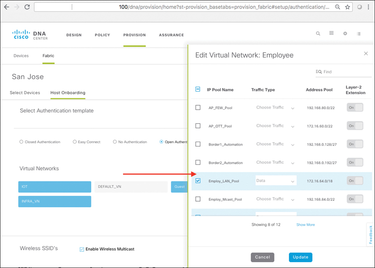
Notice on the left side of the screen that various authentication types exist. These include 802.1X Closed Mode, 802.1X Open Mode, Easy Connect, and No Authentication. NoAuth is just what it sounds like—for this port type, no authentication is performed, and users attaching to each port are simply mapped by the port’s static configuration to a given IP host pool, VN, and SGT. The 802.1X modes are more sophisticated, in that they actually perform strong authentication (username/password) for an attached host using the 802.1X protocol, with an option to fall back to an open authentication mode should the 802.1X auth fail if so chosen.
Many devices today (most modern operating systems, and many end devices) support 802.1X, and this choice is obviously more secure than a static authentication option, and should be used if possible (as one of the major benefits of SD-Access is integrated segmentation, based on user/device identity). In this case, the user/device identity is authenticated by the edge switch with the AAA server (ISE), as defined earlier in the Cisco DNA Center setup.
The Easy Connect option is an interesting one; it leverages a capability within ISE to authenticate end devices using their Active Directory login and, based on this, to assign the endpoint into the appropriate network segment, similarly as if they had used an 802.1X supplicant (but without having to have an 802.1X supplicant necessarily deployed). This is useful in cases where AD may be in use, and an 802.1X rollout may not have already been done by the organization involved.
Next, remember the process for setting up the various IP host pools in the Design workflow? Here is where you would attach those subnets to the appropriate VNs, so that when users and devices attach to the fabric and get authenticated as a member of a particular VN, they would then also be dropped into the appropriate IP host pool (subnet) to receive their IP address (typically via DHCP). It is worth noting that if you were to connect to any edge switch within the fabric (say, via SSH), you would see that each switch has a local VLAN created on it, mapped into each address pool as shown, with all edge switches sharing the same virtual default gateway IP address and virtual MAC address for that subnet (thus enabling the distributed anycast default gateway capability for attached endpoints).
Now, you may again ask yourself, if all of the edge switches share the same virtual IP address (and you may have many, many edge switches deployed within a given fabric), how does DHCP work? In other words, when the DHCP relay function on the switch picks up the user’s initial DHCP_REQUEST packet and forwards this to the DHCP server, how does the DHCP server know which of the many edge switches to send the response back to? Normally this is done by referencing the Gateway IP Address (GIADDR) field in the relayed packet to both pick the appropriate subnet for IP address assignment to the host and return the packet offering this address—the DHCP_OFFER—to the client using the DHCP relay node. In other words, when the GIADDR is not unique, but is shared across many edge switches, how does DHCP operate? Good question. Let’s explore that for a bit.
In SD-Access, the initial edge switch to which the user or device is attached inserts an extra bit of information into the relayed DHCP packet that is sent up to the DHCP server. Specifically, it inserts an Option 82 field with its own unique loopback IP address inserted in this option, along with the actual user subnet inserted as usual in the GIADDR field. The receiving DHCP server then serves up an IP address to the user, as selected from the GIADDR subnet (i.e., the host pool into which the user is mapped), and returns the DHCP_OFFER packet to this address (which is not unique, but which is part of the fabric).
Importantly, the Option 82 information is simply reflected back in this DHCP_OFFER packet, unaltered (and thus including the information about which actual edge switch initially relayed the request). Once this packet arrives back at the fabric border, this DHCP Option 82 data is extracted by the border device and is used to determine which actual edge switch to send the DHCP_OFFER packet back to, after which this packet is dispatched on its way with this updated information—and the end host user or device gets its IP address. In this way, it is not necessary to update or modify the DHCP server, and yet operation of the DHCP service with a distributed anycast default gateway deployment is transparently accommodated. All of the necessary configurations to enable the appropriate handing of this operation for DHCP Option 82 are configured by Cisco DNA Center to the border devices when these borders are added to the fabric.
As you can see, there is a lot that goes on “under the hood” of the fabric deployment—but maintaining the simplicity of fabric configuration, operation, and use is always paramount as new capabilities are added to the fabric.
When you switch over to examining the wireless configuration for IP host pools, you see something similar, as shown in Figure 19-55.
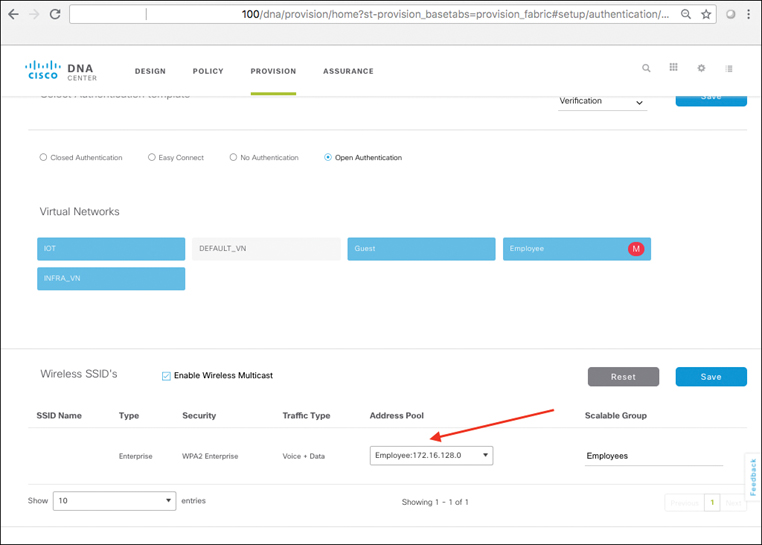
Here, you can see the defined fabric-enabled SSID (again, obscured for security reasons), along with the type of wireless security mode deployed, the traffic types involved, and the IP host pool mapped to this SSID. Also note that users in this SSID are by default mapped into the Employees group, and that wireless multicast is enabled.
Finally, let’s examine configurations all the way down to individual fabric switches and switch ports, as shown in Figure 19-56.
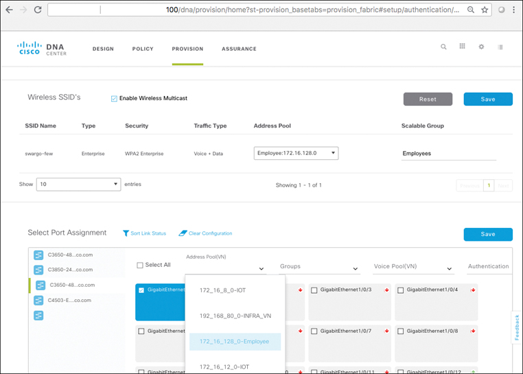
On the left side, we can observe individual switches within the fabric deployment, and as shown you can select into any individual switch and choose to view and configure all of the ports on the switch, or any individual port or group of ports, to be assigned to a particular host pool (mapped to VN), group (SGT), or authentication type (Closed Auth, Open Auth, Easy Connect, or No Auth). In this way, you have fine-grained control all the way down to the individual port level to determine how endpoints are able to attach to the fabric network, what security method they will use when they do attach, and where and how they will be mapped into the fabric network (statically via port assignment, or dynamically via AAA-delivered attributes associated with the endpoint’s login).
SD-Access Case Study, Summing Up
There are so many areas to explore within SD-Access and Cisco DNA Center that going through them all here would be an entire book in and of itself! However, hopefully this case study served to at least briefly outline how the concepts introduced earlier in this chapter—fabric overlays and underlays, the various node types (border, control plane, and edge), host pools, distributed anycast default gateways, and the like—come together and are provisioned and managed as a single, cohesive, and simple system using Cisco DNA Center.
In the “Further Reading” section, you will find a number of excellent references that will allow you to dive deeper into both Software-Defined Access and Cisco DNA Center and examine in even greater detail how SD-Access can be defined, provisioned, deployed, and managed to meet the existing—and future—goals of your organization for network segmentation, security, and simplification.
Summary
This chapter covered the following:
The challenges of enterprise networks today
An overview of Software-Defined Access as a fabric for the enterprise
A detailed examination of the capabilities and benefits of Software-Defined Access
An SD-Access case study illustrating how these capabilities can be deployed in practice
To recap, the Cisco Software-Defined Access solution introduces many key new features that, taken together, serve as a foundation for a revolution in how enterprise networks are designed, deployed, and operated. SD-Access addresses both wired and wireless deployments and, working with Cisco DNA Center and ISE, provides a solution that seamlessly integrates security, segmentation, and group-based policy enforcement in a fully automated way and with powerful monitoring and assurance capabilities.
Figure 19-57 summarizes some of the key elements and aspects of SD-Access.
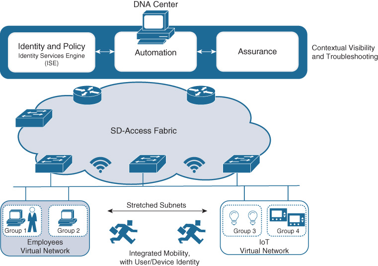
By leveraging Cisco DNA Center for simplified automation and sophisticated analytics and assurance capabilities, SD-Access provides a true next-generation set of network capabilities and forms the underpinning for an entirely new approach to enterprise networking—one that supports the requirements of modern organizations for speed, simplicity, and sophisticated, secure functionality.
As much ground as was covered in this chapter, you have only begun to scratch the surface of what SD-Access offers. If you’d like to dig deeper, a good place to start is with the items noted in the “Further Reading” section that follows.
Also note that SD-Access as a solution is continuing to evolve—and to evolve rapidly. Accordingly, there are many new functions and capabilities that, by the time you read this text, may already have been introduced for SD-Access and may be available for your use. This chapter focused mainly on the core functionality of SD-Access, items that are part of the base level of the solution and are fundamental to understand as you consider implementing SD-Access in your own network.
However, be sure to keep a sharp lookout for these new capabilities as they appear, as many of them will serve to extend the reach, functionality, and depth of the Software-Defined Access solution in exciting new ways. We are only at the beginning of the SD-Access lifecycle!
As you move on from SD-Access to the next topic area, keep your eye on SD-Access! It will continually evolve for quite some time to come, helping to drive many more new and useful innovations in the area of enterprise networking.
Further Reading
Cisco Systems Software-Defined Access portal: https://www.cisco.com/c/en/us/solutions/enterprise-networks/software-defined-access/index.html.
As noted in the chapter summary, SD-Access as a solution is only at the beginning of its lifecycle, and many new and advanced capabilities are being added to the solution constantly. Bookmark this URL and check it frequently to keep abreast of the latest developments.
Hill, C., et al. Cisco Software-Defined Access: Enabling Intent-Based Networking. Cisco Systems eBook. https://www.cisco.com/c/dam/en/us/products/se/2018/1/Collateral/nb-06-software-defined-access-ebook-en.pdf
This is a comprehensive, yet concise, introduction to SD-Access capabilities and benefits and a deeper dive into the details of SD-Access design, deployment, and operation, created by some of the same authors of this book but published in an e-book format.
Cisco Validated Design Guides
Cisco Validated Design (CVD) guides for all aspects of system design, including Cisco DNA and Cisco SD-Access, are available at the Cisco Design Zone: https://www.cisco.com/c/en/us/solutions/design-zone.html. CVDs provide authoritative Cisco guidance for best practice deployments and serve as a valuable reference as you delve deeper into the Software-Defined Access solution.
Cisco DNA–specific CVDs and other resources are available at the following URL: https://www.cisco.com/c/en/us/solutions/design-zone/networking-design-guides/digital-network-architecture-design-guides.html
The following are CVDs specific to SD-Access (as of this writing):
Software-Defined Access Design Guide (August 2018) https://www.cisco.com/c/dam/en/us/td/docs/solutions/CVD/Campus/CVD-Software-Defined-Access-Design-Guide-2018AUG.pdf
SD-Access Segmentation Design Guide (May 2018) https://www.cisco.com/c/dam/en/us/td/docs/solutions/CVD/Campus/CVD-Software-Defined-Access-Segmentation-Design-Guide-2018MAY.pdf
Software-Defined Access Deployment Guide (April 2018) https://www.cisco.com/c/dam/en/us/td/docs/solutions/CVD/Campus/CVD-Software-Defined-Access-Deployment-Guide-2018APR.pdf