7

FROM GREENHOUSE TO ICEHOUSE

A VANISHED GREENHOUSE WORLD

Antarctica was once covered with tropical forests…The…story starts in much warmer climes…in the early Eocene. Back then, the climate was subtropical, the verdant landscape dominated by palms and trees such as the monkey puzzle. By the early Oligocene, around 31 to 33 million years ago, the palms and monkey puzzles had disappeared. They gave way to more temperate species, including Huon pines…living fossils that still thrive in New Zealand and Tasmania. For trees, the transition from the Oligocene to the Miocene 23 million years back was the beginning of the end…But the end for all greenery came around 12 million years ago, when even the tundra disappeared.

—Andy Coghlan, New Scientist (2016)

Alligators, primitive hippopotami, and primates once roamed a lush, subtropical, swampy, forested, ice-free Arctic during the early Eocene Epoch, 56 to 50 million years ago (appendix C). Near the poles, surface oceans were a mild 20°C (68°F), tropical surface waters a sultry 35°C (95°F).¹ Atmospheric CO₂ soared to two to four times the pre–Industrial Revolution level of 280 parts per million (ppm).² In the absence of ice-covered poles, sea level climbed up to 70 meters (230 feet) above that of the present.

Since that climax of Cenozoic warmth, the Earth’s climate has slowly but inexorably descended into an “icehouse” world, beginning with a fairly abrupt cooling event around 34 million years ago. This signaled the first significant ice accumulation in Antarctica. Nevertheless, small, isolated glacier and ice fields may have graced the southernmost continent even earlier. The icehouse world has lasted until the present, but that may be beginning to change, as the next chapter will show. Some day we may even return full cycle back to the hothouse Eocene. But before contemplating such a return, we first explore the origins of the icehouse climate that produced the cryosphere.

DESCENT INTO THE ICEHOUSE WORLD

Birth of the Antarctic Ice Sheet

A 34-million-year event halfway through the Cenozoic Era marks a major climate transition—the initial entry into an icehouse world. Atmospheric CO₂ levels declined below critical thresholds of roughly 750 to 600 ppm.3 Large ice masses built up in East Antarctica, precipitating a 50- to 60-meter (164- to 197-foot) drop in sea level, while the surrounding ocean cooled by several degrees.⁴ But even at this early stage, the nascent ice sheet demonstrated signs of mobility. Cores drilled into sediments beneath the ice cover on the Ross Ice Shelf record multiple advances and retreats of the West Antarctic Ice Sheet (WAIS) between 23 and 14 million years ago. Atmospheric CO₂ levels fluctuated between around 280 ppm during cold periods and more than 500 ppm during warm ones, within this time interval.⁵ The climate ameliorated briefly around 23 million years ago and again 17 to 14 million years ago.

Between 34 and 23 million years ago a lowland cold temperate forest and shrub vegetation similar to modern Tasmania and New Zealand still covered the Wilkes Land margin of East Antarctica. At higher elevations, southern beech and conifers flourished in a cold tundra shrubland.6 The woody sub-Antarctic vegetation occupied a partially ice-free environment until 14 million years ago. Further cooling pushed the surviving vegetation to lower elevations until only tundra survived. After 14 million years ago, glaciers overrode the last remnant plants and turned Antarctica into a white desert. Once frigid polar conditions set in, Antarctica remained locked in the icehouse, even when climates ameliorated elsewhere.

Burial of the Gamburtsev Mountains

The Gamburtsev mountains are probably older than 34 million years and were the main centre for ice-sheet growth. Moreover, the landscape has most probably been preserved beneath the present ice sheet for around 14 million years.

—Sun Bo, Nature (2009)

The Gamburtsev Mountains, a range 2,400 meters (7,900 feet) in elevation at the center of the present East Antarctic Ice Sheet, lie entombed beneath 1,600–3,000-meter (5,250–9,800-foot)-thick ice.⁷ Discovered in the 1950s, their true nature only became apparent decades later, after ice-penetrating radar and other modern probes exposed their hidden traits (see also chap. 6). The well-preserved mountains still retain topographic features inherited from a period before the ice came, while other features represent progressive stages of the ice buildup. Deep valleys form a dendritic network like that etched by rivers in mountainous terrain. Glaciers later took advantage of these preexisting troughs. They also sculpted cirques high up near the peaks and produced hanging valleys that overlooked the main valleys, forming a landscape not unlike that of the European Alps (see fig. 4.2). The ice gradually built up in three main stages. Initially, ice only occupied cirques—hollows along the mountain crests. But as ice continued to pile up, glaciers spilled into the valleys and gouged their flanks and floors into their characteristic U-shape. Over tens of millions of years, more and more ice accumulated until it completely buried the mountains.

These stages mirror the growing ice buildup in Antarctica. Andy Coghlan, writing in New Scientist, depicted an ice-free Antarctica during the peak Eocene greenhouse, in which palm trees, araucarian conifers,8 and beech forest thrived in a subtropical coastal climate, while temperate forests occupied higher elevations. As Antarctica chilled, Alpine-style cirques and mountain glaciers gradually appeared at the highest elevations. By 34 million years ago, temperatures had cooled enough for glaciers to expand and coalescence into the first massive ice sheet on East Antarctica. Nevertheless, summer temperatures still remained above freezing. Beyond a critical threshold, 14 million years ago, when hypercold conditions set in, the ice sheet expanded to near-present dimensions, frozen to its bed. This blocked significant glacial erosion, which helped to preserve the preexisting topography.

Further Cooling

During the Pliocene Epoch, 5.3 to 3 million years ago, the WAIS expanded and contracted repeatedly.⁹ These climate cycles, lasting roughly 40,000 years, marched in step with the changing tilt of the Earth’s rotation axis—the obliquity cycle (see box 7.1). Sediments were deposited in the Ross Sea of Antarctica during warmer periods of open water with little or no sea ice. Some accumulated later beneath an ice shelf, as happens today. Sediments were absent when an advancing ice sheet rested directly on the seafloor. However, the region enjoyed a prolonged period of benign climate and ice-free open water between 3.6 and 3.4 million years ago, when the WAIS probably deglaciated completely.

BOX 7.1: THE ASTRONOMICAL THEORY OF THE ICE AGES

Milutin Milankovitch (1879–1958), a Serbian geophysicist and mathematician, proposed that an ice age starts when high-latitude summers remain cold enough to prevent the previous winter’s snowfall from melting completely. The tilt of the Earth’s axis (the obliquity)—the angle between the rotational axis and the perpendicular to the plane of the orbit (the ecliptic)—controls the amount of solar energy that reaches the top of the atmosphere. Currently 23.5°, this angle varies between 22°and 24.5° over a 41,000-year cycle. The greater the tilt when the Earth’s axis points more directly at the sun, the more intense the rays that bathe high latitudes in summer and the more snow and ice melt. Once water freezes in winter, colder temperatures no longer matter. Spring and summer thaw is more important. Conversely, a smaller tilt angle produces cooler summers and milder winters, though not mild enough to melt snow or ice. Thus, onset of glaciation is favored by a low tilt angle combined with maximum distance from the sun at the Northern Hemisphere’s summer solstice (i.e., cooler northern summers). The obliquity effect is strongest at higher latitudes, and therefore the amount of solar radiation at 65°N is considered critical to the start (or end) of a glacial cycle. Precession of the equinoxes combines two elements: (1) axial precession—a wobble like that of a spinning top, caused by the gravitational pull of the moon on the Earth’s equatorial bulge, which repeats every 26,000 years; and, more importantly for past climates, (2) elliptical precession, which determines the season when Earth is closest or farthest from the sun (perihelion or aphelion, respectively). This varies over a 22,000-year cycle. Eccentricity (100,000-year variations in the circularity of the Earth’s orbit around the sun) produces only minor changes in the total solar radiation input. However, a greater orbital elongation combined with favorable alignment of obliquity and precession may nudge the Earth enough to push it into or out of an ice age. The recipe for an ice age is outlined schematically in the following sections.

BOX FIGURE 7.1A

Precession of the equinoxes. Top: Perihelion (closest approach to the sun) occurs today near the Northern Hemisphere winter solstice. Bottom: Perihelion 11,000 years ago occurred at the summer solstice. (After John Imbrie; fig. 4.6 in Gornitz [2013])

BOX FIGURE 7.1B

Obliquity (tilt of axis) and latitudinal distribution of sunlight. Top: Today (tilt angle 23.0°). Middle: Near-zero tilt: Even latitudinal distribution favors an ice age. Bottom: High tilt angle favors a deglaciation. (After John Imbrie; fig. 4.7 in Gornitz [2013])

Recipe for Starting an Ice Age

Low Northern Hemisphere tilt angle (obliquity) + aphelion at June 21, summer solstice (precession) + highly elongated orbit (greatest eccentricity)

Recipe for Ending an Ice Age

High Northern Hemisphere tilt angle + perihelion at June 21 + highly elongated orbit

Initially greeted with great skepticism, the astronomical theory—the pacemaker of the ice ages—received a tremendous boost after the discovery of quasi-cyclical peaks at 100,000, 42,000, and 23,000 years in oxygen isotope ratios of tiny marine fossils. These periods correspond to the eccentricity, obliquity, and precession cycles, respectively. But the dominance of the 100,000-year eccentricity cycle, which should have been the weakest, remains puzzling. Clearly, other feedback processes must amplify the orbital signals; among these are the ice-albedo feedback and the greenhouse gases carbon dioxide (CO₂) and methane (CH₄), which vary in sync with the ice ages.

This period of peak Pliocene warmth offered fleeting memories of a fading greenhouse world. Atmospheric CO₂ levels were comparable to today’s (~400 parts per million), while global temperatures were around 2–3°C (3.6–5.4°F) higher. Sea level during warm intervals could have climbed up to 20 to 25 meters (66–82 feet) above present levels.10 However, the upper estimates remain uncertain because of as-yet-unresolved issues concerning regional land uplift, glacial isostatic adjustments, and gravitational attraction.¹¹

The subsequent cooling and onset of continental-scale Northern Hemisphere glaciation around 3 million years ago set the stage for a full icehouse world. The latter part of the succeeding Quaternary Period—the last 2.6 million years of Earth history—featured the periodic waxing and waning of both polar ice sheets.

Looking Closer

Some temperature changes have occurred without carbon dioxide changes, and some carbon dioxide changes have occurred without temperature changes because other factors were more important. But carbon dioxide has been important, and there is no good way to explain the ice-age cycles without appealing to the importance of the carbon dioxide.

Richard Alley, The Two-Mile Time Machine (2000)

Over the 65-million-year-long Cenozoic Era, the slow breakups and collisions of tectonic plates have shaped the Earth’s protracted descent into an icehouse world. Some key milestones include the breakup of Pangaea, the collision of the Indian plate with Eurasia, the rise of the Himalayas and Tibetan Plateau, the closure of the Tethys Ocean, and the opening and closing of critical ocean “gateways.” These latter tectonic events reconfigured ocean circulation patterns and enabled ocean currents to transport heat and moisture to the poles. Falling atmospheric CO₂ levels also intensified the global cooldown (see “The Icehouse World,” later in this chapter).

Starting 180 million years ago, the supercontinent Pangaea began to break apart, opening the North Atlantic Ocean between southeastern North America and West Africa (fig. 7.1). This was followed by the opening of the South Atlantic around 140 million years ago, and the separation of Africa, Australia, Antarctica, and India. India slowly drifted north toward Eurasia, with which it collided around 50 million years ago. Antarctica moved toward the South Pole. The Tethys Sea that once had separated Africa from Eurasia began to close as several Southern Hemisphere plates drifted gradually northward. The collision of the Indian plate with Eurasia led to the uplift of the Himalayas and the Tibetan Plateau.

FIGURE 7.1

Breakup of supercontinent Pangaea and the changing positions of the tectonic plates. (USGS)

This massive tectonic reorganization not only altered the topography, but induced major changes in the world’s climate and ocean circulation. During the early Cenozoic greenhouse, the Earth basked under high temperatures and elevated atmospheric CO₂ levels, but later, the planet cooled as CO₂ levels began to drop. How? The rise of the Tibetan Plateau (close to 5 kilometers, or 16,000 feet) intensified the summer monsoons.12 Nevertheless, a stronger Asian monsoon may not have sufficed to jump-start the growth of large ice sheets in both hemispheres. Marine geologists and paleoclimatologists Maureen Raymo and William Ruddiman therefore proposed that mountain building and faulting delivers fresh silicate rocks to the surface and exposes them to weathering by atmospheric CO₂.¹³ Carbon dioxide reacts chemically with silicate minerals in rocks and transforms them into carbonates and silica. This chemical weathering sequesters the greenhouse gas CO₂, thereby cooling the Earth, causing expansion of ice, and lowering sea level. Carbon-rich organic matter in delta, estuary, and continental shelf sediments thus faces exposure to erosion and weathering. Oxidization of the organic matter regenerates CO₂, which offsets some of the cooling. Furthermore, the same tectonic forces that pushed up the Himalayas also create volcanoes, which release fresh CO₂ into the atmosphere. This replenishes some of the CO₂ consumed by weathering. Thus, volcanic activity saves the Earth from freezing. Climate plays a delicate balancing act between these opposing forces.

Geoscientists Dennis Kent and G. Muttoni believe alternatively that the collision of the Indian plate with Eurasia around 50 million years ago brought a vast expanse of 65-million–year-old basaltic lavas—the Deccan traps sitting atop the Indian plate—to the hot, humid tropical zone. There, intense tropical weathering removed atmospheric CO₂, as described in the previous paragraph.¹⁴ The “silicate weathering machine” was in now high gear! This atmospheric CO₂ drawdown was reinforced by eruption of Ethiopian basaltic lavas 30 million years ago, after the Deccan traps had exited the tropical zone. Volcanically active Indonesia, Borneo, and New Guinea furnished additional basaltic rocks for chemical weathering. Either way, by weathering of the high Himalayas or of volcanic rocks, the atmospheric CO₂ levels dropped, the climate cooled, and the Earth continued its descent into the icehouse world.

The moving tectonic plates not only raised lofty mountain ranges, but opened and closed key ocean “gateways” that significantly altered ocean circulation with important climatic consequences. With the closure of Tethys and expansion of the Atlantic, ocean circulation gradually reoriented from a mainly east-west to a north-south direction. Although various dates have been proposed for the initial opening of the Drake Passage between Antarctica and South America in the south, a deep enough passageway had developed by 34–30 million years ago to allow currents to flow freely eastward.15 The Tasmanian Passage between Antarctica and Australia also opened around 34 million years ago.¹⁶

These gateway changes may have sparked the development and strengthening of the Antarctic Circumpolar Current (ACC) (fig. 7.2; see also chap. 6). The formation of the powerful ACC may have effectively led to isolation of Antarctica from warmer waters and cooling of the Southern Ocean, which may have set the stage for the massive ice buildup in Antarctica. Much later, another gateway, the Central American Seaway that once separated North and South America, began to shoal around 4.6 million years ago, and finally closed within the last three million years. This further restricted east-west ocean circulation and intensified the Gulf Stream, which by delivering more warmth and moisture to high latitudes would have fed the growth of Arctic ice sheets.¹⁷

FIGURE 7.2

The Antarctic Circumpolar Current. (After B. Diekmann [2007])

However, the poleward drive of heat and moisture may not have sufficed. The ACC may have intensified well after an initial Antarctic ice buildup. Computer simulations of past climate and ice sheet behavior further suggest that the ACC (and other gateways) strengthened along with the lowering of CO₂ levels, which increased cooling and glaciation.18 Diatoms, a type of free-floating marine algae (see box 7.2), would also have proliferated, nourished by the upwelling of nutrients in a vigorous ACC. Photosynthesis by diatoms would have extracted CO₂ from the atmosphere, as would have burial of organic debris in deep-sea sediments.

Marked changes in CO₂, ice sheet volume, and sea level closely accompany major Cenozoic climate transitions.¹⁹ During the torrid Eocene greenhouse, CO₂ levels reached beyond 1,000 ppm; sea level was 60 to 70 meters (197–262 feet) higher than the present level. Computer simulations show significant ice mass accumulations only when CO₂ drops below 750 to 600 ppm.²⁰ The models also suggest that enough CO₂ declined by the Oligocene, 34 million years ago, to grow an East Antarctic Ice Sheet and lower sea level by 50–60 meters (164–197 feet). During a brief climate respite between 17 and 14 million years ago, CO₂ surpassed the present-day value of ~400 ppm.²¹ But by the mid- to late Pliocene, around 3 million years ago, CO₂ levels attained near-modern values, although temperatures still remained 3–4°C (5–7°F) higher globally, even 10°C (18°F) higher near the poles.²² Sea level may have climbed over 20 meters (66 feet) above that of the present.²³ However, CO₂ had to plunge still lower—to near-preindustrial levels (~280 ppm)—before massive ice sheets appeared in the Northern Hemisphere by around 2.8 million years ago.²⁴ The development of major ice sheets at both poles marks the entry into a full icehouse world.

THE ICEHOUSE WORLD

When Greenland Turned White

Greenland really was green! However, it was millions of years ago. Greenland looked like the green Alaskan tundra, before it was covered by the second largest body of ice on Earth.

—Dylan Rood, Imperial College London

Naming “Greenland” may have been clever real estate promotion on the part of the Viking chieftain Erik the Red to lure fellow Norsemen to this barren land, but a time once existed when the name was quite apt, many millions of years ago. But the timing of onset and the size of the initial Greenland Ice Sheet remain enigmatic. As early as 38 or even 46 million years ago, a few glaciers, descending from mountain valleys, disgorged debris-laden icebergs into the ocean. By 3 million years ago, a small ice sheet probably encased portions of eastern Greenland.

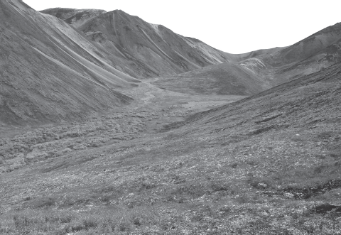
Yet as recently as 2.7 million years ago, Summit, site of a permanent research station at the highest point near the center of the Greenland Ice Sheet, was still tundra. At that time, much of Greenland may have resembled northern Alaska, where a variegated carpet of low shrubs, dwarf willow and birch, sedges, mosses, lichens, grasses, and flowers splash a bright rainbow of colors across the tundra landscape during a brief two-month-long growing season (fig. 7.3).

FIGURE 7.3

Tundra landscape, Neacola Mountains, near Big Valley, Alaska. (U.S. National Park Service/L. Wilcox)

At Summit, the bottom 13 meters (43 feet) of a 3,000-meter (10,000 foot)-long ice core is laden with silt, organic material, fossil microorganisms, trapped gases, and a water isotope composition that indicates once-warmer conditions. Paul Bierman, head of a team of U.S. geoscientists studying the silt, describes it as an “organic soil that has been frozen to the bottom of the ice for 2.7 million years.”25 The soil contains unusually high concentrations of radioactive ¹⁰Be isotopes, created when cosmic rays interact with the atmosphere.²⁶ Bierman and associates speculate that the soil must have been exposed to cosmic rays for at least 200,000 years and perhaps over a million years—far longer than the longest interglacials of the last few million years. Since the soil obviously formed before its burial under ice, the abundant cosmogenic isotopes demonstrate a long-lived, stable Greenland Ice Sheet, at least at this elevated interior location. Once the ice engulfed central Greenland, it became ensconced there and has remained ever since.

Another group of glaciologists and geologists headed by Joerg Schaefer of the Lamont-Doherty Earth Observatory at Columbia University reached a quite different conclusion. They measured the cosmogenic ¹⁰Be and ²⁶Al isotopes, this time in pieces of granitic bedrock from the base of the very same core investigated by Bierman’s team. They, too, found a long-lasting ice-free period of 280,000 years followed by at least 1.1 million years of ice cover. But this is just one of several possible scenarios consistent with the data. A number of shorter ice-free episodes lasting several thousand years, presumably during major interglacials, also fit the observed data. Since the elevated interior location of the Summit ice core would be one of the last areas to melt in Greenland, leaving only small ice cap remnants, this implies that 90 percent of the ice sheet would have disappeared. Richard Alley, a glaciologist from Pennsylvania State University and a coauthor in the Schaefer study, does not claim that therefore “tomorrow Greenland falls into the ocean. But the message is, if we keep heating up the world like we’re doing, we’re committing to a lot of sea-level rise.”²⁷

Bierman and his colleagues more recently investigated the history of these cosmogenic isotopes in offshore marine sand grains eroded from eastern Greenland’s interior by tidewater glaciers. They made note of a major ice sheet expansion 2.5 million years ago. But consistently low ¹⁰Be concentrations over the last million years imply the persistence of a large, stable ice sheet in eastern Greenland through even the longest, most intense interglacials. They maintain that the new evidence reinforces their earlier conclusion of a stable, long-lived Greenland Ice Sheet. However, other evidence points to greater mobility, at least along the flanks of the ice sheet.

Spruce and pine forests evidently thrived in southern Greenland during especially warm interglacials, such as those that occurred around 400,000 and 125,000 years ago. The former interglacial stands out because of its prolonged, near-30,000-year duration (395,000 to 424,000 years ago). Abundant spruce and pine pollen grains recovered from offshore marine sediments point to widespread boreal (northern) forests and therefore a substantially smaller southern Greenland Ice Sheet.28 Sea levels then were also higher than present. The 125,000-year interglacial also enjoyed milder climates and higher-than-present sea levels, as described in the following section.

The Ebb and Flow of the Ice Sheets

Even after Greenland turned white, the Earth continued to cool. A transitional period, roughly 1.2–0.9 million years ago, demarcated the onset of the major ice ages that have dominated the last million years. Much of what we know about these sweeping climatic oscillations comes from the heart of Antarctica, buried deep within the ice.

The ice core archives store a lengthy history of changing Earth climates. They tell a tale of at least eight major ice ages that punctuated the last million years (fig. 7.4; box 7.2). During each successive ice age peak, massive sheets of ice rolled across most of Canada into the northern United States and across Scandinavia, the British Isles, and northwestern Russia. A heavy mantle of ice blanketed all the lofty mountain ranges of the world. Each glacial-interglacial cycle lasted roughly 100,000 years, interspersed with shorter episodes of diminishing temperatures that hit rock bottom when ice sheets had expanded to their maximum extent, with a concomitant drop in sea level (note the sawtoothed-shaped curves in fig. 7.4). The cycle terminated abruptly, geologically speaking, with a rapid rise in temperature and sea level and fall in ice volume. Intervening thaws and high–sea level stands typically lasted only 10,000 to 30,000 years—just a small fraction of the entire glacial-interglacial cycle.

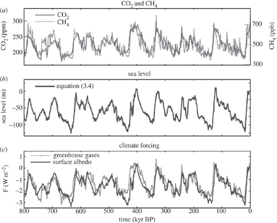
FIGURE 7.4

Sea level, temperature, and CO₂ over the last eight glacial-interglacial cycles. Note the relatively rapid rise in climate warming, sea level, and greenhouse gases following an ice age (top) as compared to the more episodic, gradual return to full ice age conditions (bottom), creating a sawtoothed-shape curve. (Hansen et al. 2013)

The repetitive, sawtoothed pattern of the ice cores is mirrored in ocean sediments. Oxygen isotope ratios of marine foraminifera (box 7.2) tell a tale of cyclically varying ocean temperatures, ice volume, and sea level. The asymmetric curves imply that the entry into each ice age—the ocean cooling, ice sheet buildup, and associated fall in sea level—was much slower than the exit, characterized by rapidly rising temperatures and sea level.

These major ice sheet and sea level oscillations also match changes in global temperature and greenhouse gases remarkably well.²⁹ The close associations illustrate the ability of CO₂ to amplify the weak 100,000-year eccentricity signal into one of recurrent glaciations or deglaciations. Nevertheless, as the weakest of the three major orbital cycles (box 7.1), the predominance of the 100,000-year cycle within the last million years and the rapidity of the retreats have long remained puzzling—until recently.

Prior to the mid-Pleistocene transitional period, the ebb and flow of glaciers had marched largely to the beat of the 41,000-year obliquity cycle, with weaker precessional influence. Signs of 41,000-year cycles preserved in the oxygen isotope ratios of tiny deep-sea fossils correspond to alternating colder and warmer periods (box 7.2). Unexplained is how these late Pliocene–early Quaternary obliquity-dominated cycles transformed into a 100,000-year, eccentricity-driven beat within the last million or so years. These cycles grew progressively longer and stronger by 900,000 to 650,000 years ago. Cold periods got even colder, suggesting that Northern Hemisphere ice sheets, in particular, thickened and spread out farther south than before.

A possible solution to the mystery, according to one hypothesis, lies in a positive reinforcement between the eccentricity and precession cycles, enabled by the vast extent of the North American continent and the southernmost reach of the spreading Laurentide Ice Sheet in North America.³⁰ As mentioned in chapters 4 and 5, the weight of a thick ice sheet depresses the land beneath it, creating a sort of bowl. Liberated of its load when the ice retreats, the formerly glaciated land rebounds. However, the actual uplift lags behind the receding ice. Due to the temporary sag, more ice lies at lower elevations within the ablation zone where melting occurs. This accelerates the pullback. The ice sheet, near the southern margin at its maximum extent, becomes sensitive to even minor climate perturbations that could initiate a retreat (or advance). Obliquity, in this scenario, merely enhances (or lessens) the summer melting that thrusts the ice sheet into a full deglacial (or glacial) mode.

During the transitional period, the temperature contrast between warm and cold periods was smaller than in later cycles.³¹ Following the transition, warm periods grew warmer, while glacial periods changed little.³² Perhaps by then Northern Hemisphere glaciations had accumulated a critical mass of ice that could bypass the obliquity signal to begin the next warming. Maybe only after several obliquity cycles passed could the feedback mechanisms (e.g., the glacial isostatic and ablation feedbacks, among others) strengthen enough to force the ice sheet into the next deglaciation. This apparently recurred on average every 100,000 years. If so, the 100,000-year beat may be merely fortuitous—only weakly related to the eccentricity cycle.

The Last Interglacial culminated around 125,000 years ago. Starting 116,000 years ago, the door to the last ice age began to open. As in previous cycles, the renewed cold initiated a series of temperature, greenhouse gas, and sea level oscillations that plunged successively lower and lower to a minimum during the Last Glacial Maximum around 23,000–19,000 years ago. With Northern Hemisphere summer insolation at a minimum, the northern ice sheets expanded across North America and Europe and sea level quickly dropped. By 20,000 years ago, the orbital cycles had locked into phase for another deglaciation. Ice sheets pulled back and sea levels rose. The last great meltdown was under way.

We scrutinize several of these events more carefully to better understand how ice sheets may affect sea level in a warming world. Two interglacials, at roughly 400,000 and 125,000 years ago, stand out because of higher-than-present sea levels. In addition, we investigate the great meltdown that ended the last ice age.

BOX 7.2: READING THE PAST

Ice doesn’t just keep a record of dust, volcanic ashes and the other subtle changes in atmospheric chemistry that together give us our weather. It has an extra property that belongs to no other history book on Earth. Living as it does on a perpetual knife edge between solid and liquid, strong and weak, ice is sensitive enough to capture tiny pockets of air, and strong enough to keep them.

—Gabrielle Walker, Antarctica: An Intimate Portrait of a Mysterious Continent (2012)

The Past as a Key to the Future

Key questions facing us are these: How much and how fast will the Greenland and Antarctic ice sheets melt? How high will sea levels rise? Current global climate and ice sheet models, while greatly improved over earlier versions, may miss important aspects of ice sheet motion that determine how fast its frigid load can be shed. Models still do not fully account for the marine ice sheet instability or the role of ice shelf thinning described in the last chapter.

Past climate analogs therefore offer an alternative means for assessing eventual outcomes, although exact comparisons may not be feasible. This longer record, extending far beyond the 100- to 150-year-long period of instrumental observations, offers a broader perspective on anticipated changes. Plausible bounds on impending ice sheet fluctuations can be set by examining past variations based on natural “archives” contained in microfossils, corals, or marine sediment chemistry and ice cores, and by studying computer climate models. A glimpse backward therefore enables us to envision oncoming ice melt scenarios and thereby to adopt more effective adaptation strategies. Here we explore two major sources of information on long-vanished periods.

Ice Core Time Capsules

The evolution of ancient climates is pieced together from diverse clues left behind by fossils preserved in land and ocean sediments, with other hints buried deep in ice and marine sediment cores. The ice cores hold an amazingly detailed account of past climate history, virtually layer by layer, year by year. The Greenland ice cores reach past the Last Interglacial to 129,000 years ago, whereas the European Project for Ice Coring in Antartica (EPICA) Dome C ice core in Antarctica yields an 800,000-year history, and a new core from the Allan Hills stretches past 1 million years.*

The ice core time capsules preserve a lengthy account of changing temperatures, atmospheric gas compositions, dust levels, and continental ice volume, among other relics of long-vanished climates. Isotopic thermometers, which exploit variations in oxygen and hydrogen isotope composition, demarcate significant milestones in paleoclimate history. Oxygen exists as several isotopes that differ only in atomic weight. The most abundant isotope, ¹⁶O, constitutes 99.8 percent of the total, with ¹⁸O a mere 0.2 percent. Hydrogen occurs as two isotopes: ordinary hydrogen (¹H, 99.98 percent) and deuterium (²H or D, 0.015 percent). Variations in ¹⁸O-to-¹⁶O ratios are expressed in parts per thousand (per mil, ‰). ¹⁸O/¹⁶O ratios can be readily measured in a wide array of materials, including glacial ice, shells of marine foraminifera, corals, cave deposits, and trees, to name just a few. Hydrogen exists in water, ice, and all living systems.

A number of natural processes can alter these basic proportions. Among the more important are evaporation or condensation of rainwater, chemical reactions, and preferential uptake of the lighter isotope by living organisms. In general, the lighter ¹⁶O and ¹H isotopes are more mobile and react faster chemically than ¹⁸O or D. When water falls as rain, the lighter isotopes remain in the cloud, whereas the heavier isotopes (¹⁸O and D) precipitate out as rainwater. As air masses migrate toward the poles, or landward, successive evaporation-condensation cycles progressively enrich rainwater in the lighter isotopes. Thus snow falling at the poles, which eventually builds up into an ice sheet, is isotopically lighter than the source ocean water. Conversely, the ocean grows increasingly heavier (i.e., enriched in ¹⁸O relative to ¹⁶O) as water is transferred to growing ice caps.

The oxygen and hydrogen isotope ratios in polar ice vary according to the local temperatures where the precipitation occurs. Other variables, such as moisture sources, topography, and season, also affect these ratios. Despite some differences, similar isotope ratio patterns from different ice cores suggest a common temperature signal. Therefore, they can serve as valid paleothermometers. For example, each 1°C (1.8°F) rise in temperature increases the O isotope ratio in Greenland ice by ~0.7‰.

The ice cores also capture tiny pockets of the atmosphere. Tiny air bubbles trapped in the ice encapsulate atmospheric greenhouse gases such as carbon dioxide, methane, and nitrous oxide. These greenhouse gases oscillated in sync with temperatures over the 800,000-year history of the EPICA ice core, rising during interglacials and falling during glacials.† Both greenhouse gases, CO₂ and CH₄, increased as temperatures rose and declined as temperatures fell (fig. 7.4). But never during the 800,000-year history of the ice cores did they approach today’s high levels.

Dustiness in ice varied inversely with temperatures. Widespread aridity gripped many parts of the Earth during frigid glacial periods. Vegetation cover shrank and deserts expanded. Stronger winds also lifted more dust off the ground. Wind-borne dust like that of the 1930s Dust Bowl swept across large swaths of North America, Northern Europe, and Central Asia. The eolian dust accumulated in extensive deposits of buff-colored, fine silt called loess. Some of this fine dust ultimately fell on the Greenland Ice Sheet. With the return of warmer and wetter interglacials, more abundant rainfall restored the vegetation; the winds subsided. Polar ice then cleared up and became almost dust-free.

Thin sulfuric acid aerosol (sulfate) and ash layers in the ice provide evidence of past volcanic eruptions. Some especially explosive eruptions that left an imprint in Greenland ice cores include Tambora, Indonesia (1815); Krakatau, Indonesia (1883); Katmai, Alaska (1912); El Chichón, Mexico (1982); and Mount Pinatubo, Philippines (1991). The largest eruptions, by injecting copious amounts of sulfate aerosols into the stratosphere (upper atmosphere), partly dimmed incoming sunlight and reduced temperatures in following years. For example, the “year without a summer” followed the Tambora eruption in 1815. Brilliant sunsets painted the sky red that year, but crops also failed and famine struck. Volcanic eruptions that maximize the global distribution of aerosols and appear in the polar ice cores tend to occur at lower latitudes.

Marine Archives

The oxygen isotopes embedded in tiny marine creatures—foraminifera‡—register sea level changes that mirror changes stored in Greenland and Antarctic ice core archives. The oxygen isotope ratios of these creatures mirror those of the water they inhabit, which in turn responds primarily to temperature and ocean volume variations. (These ratios also vary with the particular species studied and ocean salinity.) In general, ¹⁸O/¹⁶O ratios become progressively heavier at lower temperatures. They also grow heavier during glacials, when large volumes of ocean water are locked up in ice sheets, and conversely, lighter during interglacials, when the ice sheets contract and ocean volume increases. Thus, heavier ¹⁸O/¹⁶O ratios in foraminifera correspond to glacial periods and lower sea levels, and lighter ratios to interglacials and higher sea levels.

BOX FIGURE 7.2

Planktonic (free-floating) foraminifera Globigerina bulloides (left) and Dentoglobigerina altispira (right). (H. J. Dowsett, “Foraminifera,” in Encyclopedia of Paleoclimatology & Ancient Environments, ed. V. Gornitz [Dordrecht: Springer, 2009], 338, fig. F2. Reproduced by permission of Springer Nature)

However, the ¹⁸O/¹⁶O ratio embeds ambiguity, because while it mainly reflects ice volume (and hence, sea level), it also depends on water temperature. Ice volume changes account for roughly two-thirds of the glacial-interglacial isotope difference, ocean temperatures the remainder. Resolution of this ambiguity requires an independent measure of ocean temperature.

One such measure is the magnesium-to-calcium (Mg/Ca) ratio in marine carbonate shells. Magnesium readily replaces calcium as foraminifera build their calcite shells. The extent of this atomic substitution depends primarily on water temperature. A higher Mg/Ca ratio generally implies a higher temperature. Empirical Mg/Ca-temperature relationships based on living forams have been applied to their fossil ancestors. These relationships depend on the particular species examined. The Mg/Ca method enjoys an important advantage in that both the chemical and isotopic composition can be measured on the same sample.§

Other useful seawater paleothermometers include alkenones and TEX₈₆. Alkenones belong to a class of long-chain organic molecules produced by tiny, free-floating marine algae, such as coccolithophores, which are widespread throughout the world’s oceans and often produce extensive algal blooms. These algae produce alkenones with different proportions of double bonds between carbon atoms (i.e., more unsaturated carbon bonds), depending on the water temperature in which they grow. This provides a measure of past sea surface temperatures.

Biomarkers, like TEX₈₆ found in the free-floating marine organism Crenarchaeota, are also sensitive indicators of past sea surface temperatures.** The TEX₈₆ paleothermometer is based on the relative proportion of fatty cell membrane biomolecules within the organism, which readjusts the composition of these molecules in response to changing sea surface temperatures. In spite of local variations in surface currents and temperatures, average worldwide sea surface temperatures respond primarily to major global climate changes. Thus, TEX₈₆ serves as an independent means of separating past ocean temperature changes from variations in ice volume or sea level.

* NEEM (2013); Brook (2008); Higgins (2015).

† Brook (2008); Foster and Rohling (2013); Grant et al. (2012).

‡ Foraminifera (or simply, forams) are tiny, single-celled, chiefly marine organisms that can either be free-floating or dwell on the ocean floor or in brackish water. Most species have shells made of calcium carbonate, partitioned into chambers that are added during growth.

§ Higginson (2009).

** The TEX₈₆ molecule is a type of biomolecule naturally occurring in fats, waxes, and certain vitamins (e.g., vitamins A, D, E, and K). TEX₈₆ contains 86 carbon atoms. It has been found to be empirically correlated with sea surface temperature.

HOW STABLE ARE THE ICE SHEETS?

Looking Through the Mists of Time

As we have seen, ice sheets have repeatedly waxed and waned over the geologic past. The nascent Antarctic ice sheet, 34 to 32 million years ago, grew and shrank repeatedly until it attained near-modern dimensions.33 Mid-Pliocene marine archives also record recurrent West Antarctic Ice Sheet collapses.³⁴ Even the presumably stable East Antarctic Ice Sheet may have retreated during warmer episodes, at times when sediment detritus from the continental interior and fossil diatom deposits indicate ice-free, open water in Wilkes Basin.³⁵ Large global sea level oscillations paralleled these major ice sheet excursions.

Approaching the present, we zoom in on three periods within the last half million years when the ice relaxed its gelid grip and the ice sheets rolled back substantially: 400,000 years ago, around 125,000 years ago, and 20,000 years ago. Do these drastic past meltdowns foreshadow an increasingly aquatic future?

The 400,000-Year Interglacial

This warm interlude, from approximately 424,000 to 395,000 years ago, lasted nearly 30,000 years. Global temperatures resembled those of the present, although polar temperatures were several degrees higher. Atmospheric CO₂ closely matched preindustrial values of ~280 ppm.³⁶

Several geologists reportedly found remnants of 400,000-year-old shorelines 20 meters (66 feet) above present sea level on the tectonically stable islands of Bermuda and the Bahamas. However, prior researchers had neglected to consider glacial isostatic adjustments. The periphery of the North American Laurentide Ice Sheet had bulged upward, but subsequently subsided once the ice melted. Taking this subsidence into account, geoscientists Maureen Raymo and Jerry Mitrovica from Columbia and Harvard Universities, respectively, calculated a more likely, lower sea level rise of 6–13 meters (20–43 feet). They concluded that “both the Greenland and the West Antarctic Ice Sheet collapsed during the protracted warm period while changes in the volume of the East Antarctic Ice Sheet were relatively minor.”³⁷

Meanwhile, another research team, headed by Alberto Reyes of the University of Wisconsin–Madison, focused their attention on offshore marine sediments of this age from southern Greenland.38 To them, the absence of glacially eroded sediments in the south, although present farther north and east, suggested a complete deglaciation of southern Greenland—enough to raise global sea level by 4.5 to 6 meters (14.8–19.7 feet). Abundant spruce pollen grains within the sediments offered further proof of ice-free, forested areas, as noted in “When Greenland Turned White”, earlier in this chapter. The unusually prolonged interglacial and higher Arctic temperatures may have spurred the meltdown. A maximal global sea level rise of 13 meters (42.6 feet) implies crumbling of the entire West Antarctic Ice Sheet, with some minor East Antarctic breakup as well.³⁹

The Last Interglacial

The penultimate thaw between the ice ages, known variously as the Eemian in Europe and the Sangamonian in North America, lasted from approximately 129,000 to 116,000 years ago. Northern summer sunlight intensified between 130,000 and 127,000 years ago, and average polar temperatures climbed several degrees higher than today, without altering global temperatures significantly. Approaching 10 meters (33 feet) of present sea level, the ocean sped upward at double today’s rates. At its peak, sea level then stood 6 to 9 meters (20–30 feet) higher than present levels.⁴⁰

Uplifted shorelines and coral reefs in western Australia suggest the occurrence of two sea level peaks, the first +3.5 meters (11.5 feet) above present levels between ~127,000 and 119,000 years ago, and a second, higher peak up to 9 meters (29.5 feet) above present levels 118,000 years ago.⁴¹

Oxygen isotope ratios in Red Sea foraminifera also flag two sea level highs—at ~123,000 years ago and 121,500 years ago—followed by a sharp drop-off after 119,000 years ago.⁴² At its zenith, sea level may have zipped upward as fast as 2.5 meters (8.2 feet) per century. A Greenland-sized ice sheet could have disappeared within four centuries at an average sea level rise rate of ~1.6 meters (5.2 feet) per century. How much of Greenland actually disappeared remains uncertain.

A new study casts doubt whether a sea level drop separated the apparent two high peaks of this interglacial.43 After an exhaustive review of the evidence, the authors find no conclusive signs of ice-sheet regrowth and sea level drop during this period. Nor can they account for climate processes that would explain the resurgence of glaciation in the midst of an interglacial. They therefore urge caution in interpreting the proposed high rates of sea level rise following the alleged low sea level stand. Alder and fern vegetation covered southern Greenland between 127,000 and 120,000 years ago, as during an earlier interglacial. Abundant pollen and spores from these plants, as well as glacially eroded silt, were deposited offshore. These signs of vegetation point to ice-free conditions inland. Nevertheless, the reduced ice cover on Greenland raised sea level by only 1.6 to 2.2 meters (5–7 feet).⁴⁴

An international team of scientists headed by Dorthe Dahl-Jensen from the Niels Bohr Institute in Copenhagen drilled the first ice core down to the base of the Eemian during the North Greenland Eemian Ice Drilling (NEEM) project. Although the bottommost layers of the 2,500-meter-long ice core were severely crumpled, a key section spanning the period from 129,000 to 116,000 years ago yielded a wealth of information. An entire layer of Eemian-age ice had melted and refrozen, producing features similar to the widespread melt layer that covered most of the ice sheet during the great thaw of July 2012 (chap. 5). The ice core oxygen isotope paleothermometer registered temperatures 8°C (14°F) higher than present. But despite this unexpectedly high warmth, the Greenland Ice Sheet thinned by only 400 meters (1,300 feet), raising sea level a mere 2 meters (6.6 feet). “The good news,” says Dahl-Jensen, “is that Greenland is not as sensitive to climate warming as we thought. The bad news is that if Greenland’s ice sheet did not disappear during the Eemian, Antarctica must have been responsible for a significant part of the sea level rise.”⁴⁵

Aircraft flying over Greenland between 1993 and 2013 used ice-penetrating radar to delineate the interior structure of the ice sheet. This information enabled scientists to map the distribution of ice layers of different ages. A surprising result is how little Eemian or older ice still exists.⁴⁶ Old ice survives only in a fairly small patch of east-central Greenland and a larger area of northwestern Greenland. What became of the very old ice? Two possibilities exist. One is that large portions of the ice sheet containing the oldest ice disappeared during the major interglacials, such as the one 400,000 years ago, or during the Eemian. Subsequent snowfalls during glacial periods helped to rebuild the ice sheet. Most of what we see today has accumulated since the Last Interglacial. The other alternative is that very old ice at the base melts due to the high pressures and geothermal heat and escapes via subglacial streams. Fresh snowfalls make up for losses at the base, in a kind of steady state.

Although multiple lines of evidence point to a reduced Eemian Greenland Ice Sheet, how much smaller remains uncertain. Many studies suggest that Greenland added only 2 to 4 meters (6.5–13 feet) to sea level.47 Since this falls far short of the total estimated sea level rise, the West Antarctic Ice Sheet presumably made up most of the balance, with some East Antarctic contributions in the highest scenarios. To add to the uncertainty, the recent study alluded to several paragraphs above finds no signs of major sea level fluctuations during the Eemian interglacial.

Since the Earth could reach Last Interglacial temperatures later in this century, will sea level climb to Eemian heights again? Before answering this important question in the next chapter, we zoom in on the last great meltdown.

The Last Great Ice Meltdown

At the height of the last ice age 25,000 to 20,000 years ago, North America lay under a miles-thick ice sheet as far south as present-day South Dakota, Iowa, Illinois, Ohio, and Long Island. In Europe, the ice reached present-day Berlin, Warsaw, and the British Isles, and covered the Alps. New York City, too, was deeply buried in ice. Although the ice has long since vanished, the trained eye can easily spot signs of its passage. The long-gone glaciers left their calling cards throughout Central Park, a leafy oasis in the midst of bustling Manhattan. Among these are well-polished rock outcroppings, worn smooth by the overriding ice sheets and jagged on the “downstream” side; grooves or scratches gouging the rock surfaces; and exotic boulders transported by the glaciers from across the Hudson River or from upstate New York and left behind when the ice melted (see fig. 4.4). A ridge of jumbled sand and gravel slashes across Staten Island, Brooklyn, central Queens, and the middle of Long Island. This ridge represents the terminal moraine—the debris pile that marks the southernmost advance of the ice (see chap. 4).

By 20,000 years ago, as northern summer sunlight gradually strengthened, the glaciers had embarked on their northward journey. Sea level rose slowly at first. The pace quickened by 16,000 years ago, as more and more ice melted. By 14,600 years ago, the meltdown had gathered full speed and sea level rose rapidly as the trickle swelled into major torrents. After 7,000 years ago, the meltdown neared its end and sea level gradually approached its present level.

Multiple abrupt outbursts, termed meltwater pulses, punctuated the overall rise between 15,000 and 7,500 years ago (fig. 7.5; table 7.1). During the earliest spike ~19,000 years ago (meltwater pulse 1A₀), ocean levels may have sprung upward by 10–15 meters (33–49 feet) within a few hundred years.

FIGURE 7.5

Generalized curve of sea level rise after the last ice age. (After fig. 5.1b in Gornitz [2013])

TABLE 7.1   Meltwater Pulses During Periods of Rapid Sea Level Rise

MELTWATER PULSE 1A0
TIMING (YR)	RATE OF SLR (MM/YR)	INCREASE IN SEA LEVEL (M)	REFERENCES
~19,000	—	10–15	Yokoyama et al. (2000)
~19,000	≥20	10 m in ≤500 years	Clark et al. (2004)
19,600–18,800	~12.5 (average)	10	Hanebuth et al. (2009)
MELTWATER PULSE 1A
TIMING (YR BP)	RATE OF SLR (MM/YR)	INCREASE IN LEVEL (M)	REFERENCES
14,300–12,800			Stanford et al. (2011)
13,800 (peak)	~26 (max.)	—	Stanford et al. (2011)
14,650–14,300	46	16 m in ~350 years	Deschamps et al. (2012)
14,600–14,300	—	16–19	Carlson and Clark (2012)
~14,500	—	~8.6–14.6	Liu et al. (2016)
MELTWATER PULSE 1B
TIMING (YR BP)	RATE OF SLR (MM/YR)	INCREASE IN LEVEL (M)	REFERENCES
11,500–9,500			Stanford et al. (2011)
10,900; 9,500 (peak)	19; 25 (max.)	—	Stanford et al. (2011)
~10,500	26	~28	Fairbanks (1989)
11,000	~25	~13	Bard et al. (1990)
11,100–11,400	~40	~15 m (Barbados only)	Bard et al. (2010); other sites: none to small SLR acceleration
MELTWATER PULSE 1C
TIMING (YR BP)	RATE OF SLR (MM/YR)	INCREASE IN LEVEL (M)	REFERENCES
8,100–8,300	—	0.9–2.2 (range)	Carlson and Clark (2012)
8,200–8,300	—	0.8–2.2	Li et al. (2012)
7,600–8,200	~12	~6 m in ≤500 yr	Cronin et al. (2007)
~7,600	~10	~4.5 m	Yu et al. (2007)

Source: Revised and updated from Gornitz (2013), table 5.1.

The largest upward spurt, meltwater pulse 1A (MWP-1A), occurred between 14,600 and 14,000 years ago, during the milder Bølling-Allerød period, when Greenland’s temperatures climbed by 4.5°C to 9.9°C (8°F to 18°F). At its fastest, sea level leaped upward by 16 to 19 meters (54–62 feet) within 300 years, at rates of up to 46 millimeters (1.8 inches) per year (table 7.1).

Because of its vast size, the breakup of the Laurentide Ice Sheet in North America was generally assumed to dominate meltwater MWP-1A, with lesser inputs from northern Eurasia. (Greenland contributed little, given its relatively small ice volume.) Vestiges of the glaciers’ passage show that Northern Hemisphere sources accounted for at most half of the total meltwater, which leaves the door open for substantial Antarctic inputs.⁴⁸ Does the geologic evidence substantiate a significant role for Antarctica during MWP-1A?

The history of ice regression in Antarctica is less clear-cut than that in the Northern Hemisphere, owing to its remoteness, harsh climate, and limited data. In the Mac. Robertson region of East Antarctica, most sediments left by retreating ice sheets are younger than 12,000 years old, although the retreat may have begun as early as 14,000 years ago, during MWP-1A.⁴⁹ On the other hand, melting icebergs dumped embedded debris seaward of the Ronne-Filchner Ice Shelf in East Antarctica at least eight times between 20,000 and 9,000 years ago. These events likely marked early stages in the overall regional ice retreat. The most pronounced episode began around 15,000 years ago and peaked between 14,000 and 14,400 years ago, which coincides with MWP-1A.⁵⁰ However, the other events were probably too small to result in meltwater pulses. Meanwhile, on the West Antarctic Ice Sheet, Pine Island Glacier retreated to within 100 kilometers (60 miles) of its present grounding line before 10,000 years ago, although exactly when is uncertain.⁵¹ Curiously, ice in the Ross Sea region of Antarctica reached a maximum between 18,700 and 12,800 years ago, followed much later by retreat. This rules out this area as a candidate source for MWP-1A.⁵²

Can geophysics shed further light on this contentious history? Different meltwater sources (e.g., the Laurentide, Antarctic, and Barents Sea ice sheets) leave distinctive “fingerprints,” i.e., they produce different geographic patterns of sea level rise depending on how much ice melts and where. Water flows away from a dwindling ice sheet because the gravitational pull between it and the ocean weakens. In addition, the ocean level drops near ice-free land that rebounds from the decreased isostatic loading, even as the ocean gains more water overall (see chaps. 4 and 6). The calculated regional sea level signatures that best match observations suggest a substantial Antarctic input for meltwater pulse 1A.⁵³ However, remaining uncertainties still cloud the extent of Antarctica’s role in the meltwater pulse.⁵⁴

The last two meltwater pulses (MWP-1B, MWP-1C) were much weaker than MWP-1A (table 7.1). Meltwater pulse 1B—between 11,500 and 11,000 years ago—materialized upon the return of warmth after a brief relapse into the Younger Dryas neo–ice age between 12,800 and 11,700 years ago. Although fossil corals from Barbados register a distinct sea level jump, elsewhere this event appears as just a minor speedup in an overall rising trend.

Sea level sped up several times again between ~9,000 and 7,600 years ago. Meltwater pulse 1C (MWP-1C) may be related to an episode around 8,200 years ago when colder temperatures gripped Greenland, and European summers chilled by several degrees (table 7.1). The cold may have been triggered by the final catastrophic drainage of giant glacial lakes along the southern edge of the Laurentide Ice Sheet and their discharge into Hudson Bay as the last ice sheet remnants disintegrated.⁵⁵ Although the enormous influx of icy freshwater to the world’s oceans likely cooled them (and regional climates), it merely elevated sea level a few meters if spread out evenly over the ocean.

The meltwater pulses that punctuated the great meltdown were closely linked to outbursts of glacial meltwater from rapidly crumbling ice sheets and glacial lakes, although specific sources have often been difficult to pinpoint. Since the mammoth Laurentide Ice Sheet that once buried much of North America no longer exists, abruptly disintegrating ice masses may not suddenly unleash massive meltwater pulses—at least not immediately. However, we cannot rule out such an outpouring from Greenland and West Antarctica if global temperatures continue to ramp upward.

This could indeed come to pass in the far future. Having retraced the prolonged, winding path of planetary transformation from greenhouse to icehouse, we turn next to the prospect of reversing course and returning to a greenhouse world—one in which only ragged remnants of today’s cryosphere may survive. Though this radical notion may seem far-fetched today, the next chapter examines why this fanciful vision could become our everyday reality at some future date.