PROBABILITY & RISK
PROBABILITY & RISK
GLOSSARY
algorithm A mathematical or computational method used to achieve a result.
critical value A value taken from a statistical distribution as a threshold for determining whether a test statistic is more extreme or not than expected.
false positive/negative A prediction given as true when it should be false or false when it should be true.
Fermat’s Last Theorem Conjecture posed by French mathematician Pierre de Fermat in 1637, which states that no three positive integers a, b, and c satisfy the equation an + bn = cn for any integer value of n greater than 2. No proof of the Theorem existed until 1994.
Fermat’s Little Theorem Theorem that states that for a given prime number, p, and an integer, a, then ap - a is an integer multiple of p.
Fermat’s Principle of Least Time Principle that states that light will always travel between two points using the path that takes least time.
Fermat’s Two-square Theorem The set of Pythagorean primes where the prime number is the sum of two squares.
machine learning A statistical and computational algorithm that learns features from data through trial and error of known data.
null hypothesis The default assumption of an experiment that there is no relationship between the variables under observation.
objective probability The probability that something will occur based on factual or observed historical data.
petabyte A value of 250 bytes, abbreviated as PB.
subjective probability The probability that something will occur based on experience or knowledge.
PROBABILITY
the 30-second calculation
Probability provides a measurement of the chance or likelihood that a specific event will occur. The probability is calculated between 0 (no chance of occurrence) and 1 (it is certain that the event will occur). The higher the probability that the event occurs, the closer to 1 it becomes. For example, the probability of getting heads or tails on a fair coin (one which has heads and tails) is 0.5 or 50%. Probability can be viewed from largely two different perspectives. The first is objective or frequentist probability, where the probability of an event happening is described by the relative frequency of occurrence of the event in a scientifically repetitive set of experiments. This generates a number to objectively describe the probability. The second is subjective probability, the most popular of which is a Bayesian probability where expert knowledge as well as experimental data are used to determine the probability of an event occurring. Expert knowledge is determined by a prior probability which is subjective, experimental data is incorporated as a likelihood ratio and these are multiplied together to calculate odds of the event occurring. Bayesian probability is used in forensic science in the provision of expert evidence to the courts, as well as in many other applications where risk is being ascertained.
3-SECOND COUNT
Probability is a general term used to describe an area of mathematics that relates to calculating the likelihood or chance of something happening.
3-MINUTE TOTAL
The use of probabilistic analysis emerged around the mid-seventeenth century when a more precise and theoretical underpinning emerged to the concept of defining the chance of events occurring. The first textbook on probability theory was published in 1718 by Abraham de Moivre, a French mathematician.
RELATED TOPICS
See also
3-SECOND BIOGRAPHY
GEROLAMO CARDANO
1501–76
Italian polymath who was interested in the natural sciences including physics, biology and chemistry as well as mathematics; credited with being one of the key founders of what we now understand as probability
30-SECOND TEXT
Niamh Nic Daéid
Tossing a coin has a 50% probability of getting heads or tails as the outcome.

PREDICTION
the 30-second calculation
Knowing what will happen in the future would allow us to make perfect decisions. This is impossible, of course, but just being able to estimate the probability of certain events can be greatly beneficial when planning for the future. Prediction in statistics revolves around finding dependencies between variables, so that if we gain information about them now then we have a better idea about how they will behave in the future. Ideally, we do this by identifying a causal relationship and monitoring the causal factor to predict the events that it will cause. However, in the real world, it is challenging to be able to prove causality because of the large number of other changing factors that may also affect what is being measured. Machine learning attempts to make predictions by discovering complex patterns in data that would be very hard for the human brain to recognize. Petabytes of data can be processed to create and update predictions of things such as stock prices and social media trends, which is invaluable information for hedge funds and marketing companies. Since automated predictions have such an influential role in modern society, it is important for algorithm design teams to also be ethically responsible. While machines are capable of data processing on levels that humans are not, it is difficult to program simple moral rules that we take for granted.
3-SECOND COUNT
Prediction aims to determine the occurrence of future events, often using our knowledge of the past and present. It is a key goal in statistical analysis.
3-MINUTE TOTAL
An example of unintended discrimination comes in using algorithms to predict crime hotspots and an individual’s crime risk for more targeted policing. It is argued that the current use of such algorithms can encourage racial profiling without accountability and therefore must be used transparently.
RELATED TOPICS
See also
LINEAR REGRESSION & CORRELATION
3-SECOND BIOGRAPHY
JOHN GRAUNT
1620–74
English haberdasher who is credited with creating the first life table – a prediction of an individual’s survival probability for the upcoming year based on their current age
30-SECOND TEXT
Harry Gray
Information is constantly churned into models that attempt to predict the future.

HYPOTHESIS TESTING
the 30-second calculation
A statistical hypothesis is a statement about a population which may or may not be true; hypothesis testing involves testing this statement. A claim that ‘an immunization programme has reduced the measles infection rate in a community from 20%’, is an example of such a hypothesis. The researcher forms the null hypothesis – for example, ‘the infection rate remains at 20%’ – often with the aim or hope of finding enough evidence to reject this in favour of the alternative hypothesis – ‘the infection rate has decreased from 20%’. The test involves calculation of a test statistic based on sample data. This is compared to a critical value derived from a standard statistical distribution, together with a reliability requirement – the confidence level – set by the researcher. There is a trade-off between confidence in the result and its precision: absolute confidence that the infection rate lies between 0% and 100% is useless. The result of a hypothesis test may be wrong. A type I error is one in which the null hypothesis is wrongly rejected in favour of the claim in the alternative – the immunization programme is wrongly found to be effective when the infection rate is unchanged. A type II error is one in which the null hypothesis is wrongly accepted – the immunization programme has reduced the infection rate but the test concludes incorrectly that the programme does not work.
3-SECOND COUNT
Hypothesis testing uses statistical procedures to determine whether a hypothesis is true, placing the burden of proof on the researcher making the claim.
3-MINUTE TOTAL
In a courtroom the presumption of innocence is the null hypothesis and its rejection is the alternative, of guilt. In this setting, type I errors are typically more strenuously avoided than type II: ‘It is better that ten guilty persons escape than that one innocent suffer.’ (Blackstone).
RELATED TOPICS
See also
FALSE POSITIVES & FALSE NEGATIVES
30-SECOND TEXT
John McDermott
A claim that a medicine is effective is a hypothesis that may be tested.

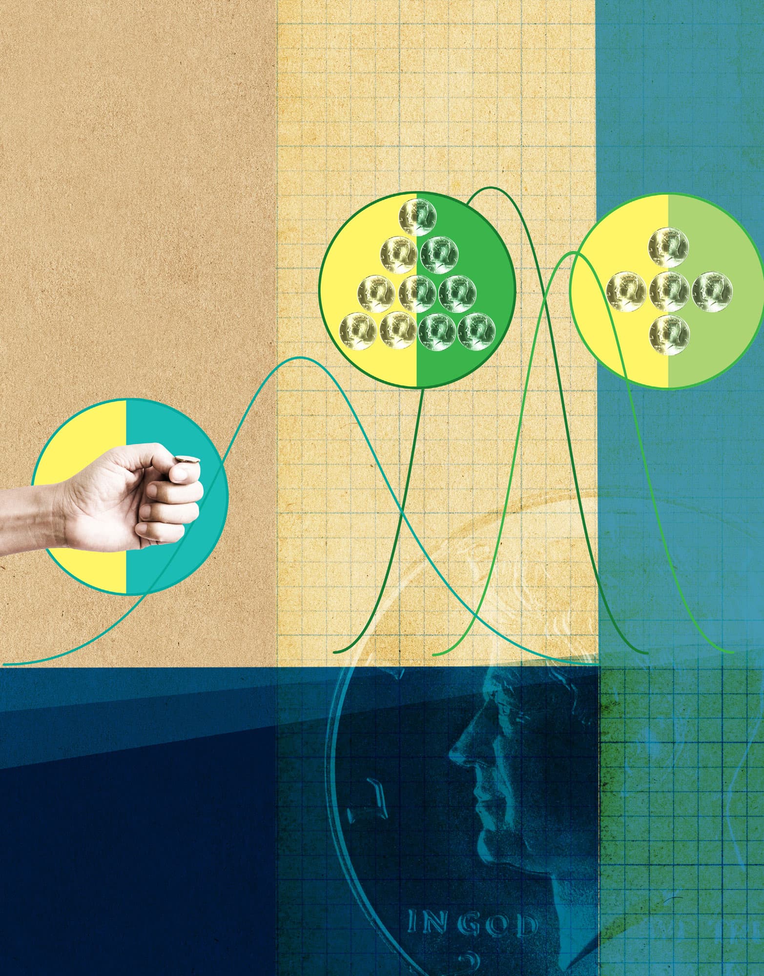
BAYESIAN PROBABILITY
the 30-second calculation
Imagine asking a room of 1,000 people if they believe that a certain coin is fair (equal chance of heads or tails) before tossing it. Most people would say yes based on what they know about the majority of coins, despite knowing nothing about this particular coin. How many people would change their mind if the coin was tossed five times and they were all heads? Some people might but others might attribute it to luck. How about ten heads in a row? Those people who swapped before ten heads would now be confident in their belief that the coin is unfair, and sceptics might have changed but still be doubtful. All of these people have their own belief about the fairness of the coin. This idea is mathematically formalized in what is known as Bayes’ theorem. Bayes’ theorem relates the conditional probabilities of two events together. Conceptually, it can be described as obtaining a new (posterior) degree of belief in an event by combining your current (prior) degree of belief with an observation of another event (evidence) – some people believe that this is the natural way that humans think and learn. Philosophically, the Bayesian idea of probability is different from what we call frequentist probability. The Bayesian versus frequentist approach to probability is a long-standing debate among statisticians.
3-SECOND COUNT
Bayesian probability can be thought of as an individual’s degree of belief in an event occurring.
3-MINUTE TOTAL
Through the Bayesian ‘prior’ degree of belief, subjective information about events can be included in statistical models to improve analysis. However, without due diligence, this subjectivity can incorporate unnecessary bias that instead leads to an inaccurate posterior belief.
RELATED TOPICS
See also
3-SECOND BIOGRAPHY
THOMAS BAYES
1702–61
English statistician whose notes on ‘inverse’ probability were published posthumously, later giving rise to what we call Bayes’ theorem
30-SECOND TEXT
Harry Gray
Our posterior belief is obtained based on the strength of prior knowledge and the observed evidence.
CONDITIONAL PROBABILITY
the 30-second calculation
It is an intuitive idea that certain events occurring can affect the chance of others occurring. Conditional probability is the formal mathematical construction to describe this intuitive idea. Situations that involve conditional probability appear frequently when playing games. Imagine a two-player dice game in which player two rolls a dice first, followed by player one doing the same. The rule is that if player two gets a higher number on their roll then they win, otherwise player one wins. Before player two rolls, their probability of winning is 5/12 (roughly 42%). Suppose player two then rolls the dice and gets a five. The probability that they will win changes to 2/3 (66%), since player one can only roll either a 5 or 6 to win. Here we have conditioned on the event that player two rolls a 5 and, in that situation, the probability of player two now winning the game increases. However, if the event that we are conditioning on is independent of the event whose probability we wish to calculate, then the conditional probability remains the same as if we hadn’t seen the other event. An example of that in the same game is if we condition on which day of the week it is. Clearly the day of the week does not affect which numbers will appear on either dice and therefore does not affect the game in any way, so the probabilities remain unchanged.
3-SECOND COUNT
Conditional probability is the probability of an event occurring while assuming that other different events have already occurred.
3-MINUTE TOTAL
The Monty Hall problem is a famous example of conditional probability. With a prize behind one of three doors, players can select one door. An empty door is opened, and the player is given the choice to switch to the other unopened door. Switching increases the player’s chance of winning.
RELATED TOPICS
See also
INDEPENDENT & DEPENDENT VARIABLES
3-SECOND BIOGRAPHY
PIERRE DE FERMAT
1607–65
French lawyer and mathematician famous for posing Fermat’s Last Theorem, a mathematical conjecture that went unsolved until 1994, when it was proven by English mathematician Andrew Wiles
30-SECOND TEXT
Harry Gray
The probability of events may change based on what we have already seen.

LIKELIHOOD RATIO
the 30-second calculation
The likelihood ratio is computed by taking the ratio of the likelihood of an event conditional on two different circumstances. If it is large, then the likelihood of the event under the first circumstance is far greater than the likelihood of the event under the second circumstance, and vice versa. It is popular in diagnostic testing where it is used to assess the utility of performing a test, since test results are almost never 100% certain. For example, suppose a test is 99% accurate at giving a correctly positive result when someone has a disease. It is also 90% accurate at giving a correctly negative result when someone does not have the disease, meaning that it will incorrectly give a positive result when someone does not have the disease 10% of the time. The positive likelihood ratio is then the ratio of the probability that the test is positive given that they do have the disease compared with the probability that the test is positive given that they don’t have the disease, which is 0.99/0.1 = 9.9. This means that if someone has the disease, then the test is 9.9 times more likely to give a positive result than if the person did not have the disease, which is reassuring for our confidence in the test. Note that the likelihood ratio has not told us the probability that the person does actually have the disease when we receive the test result.
3-SECOND COUNT
The likelihood ratio is a statistic that is used to compare the probability of an event occurring under two different circumstances.
3-MINUTE TOTAL
In 2010, the widely used method of mammography screening for breast cancer detection was estimated to have a positive likelihood ratio of 5.9 and negative likelihood ratio of 0.3 for women under 40 years old.
RELATED TOPICS
See also
FALSE POSITIVES & FALSE NEGATIVES
30-SECOND TEXT
Harry Gray
The size of the likelihood ratio updates the post-test probability of disease.

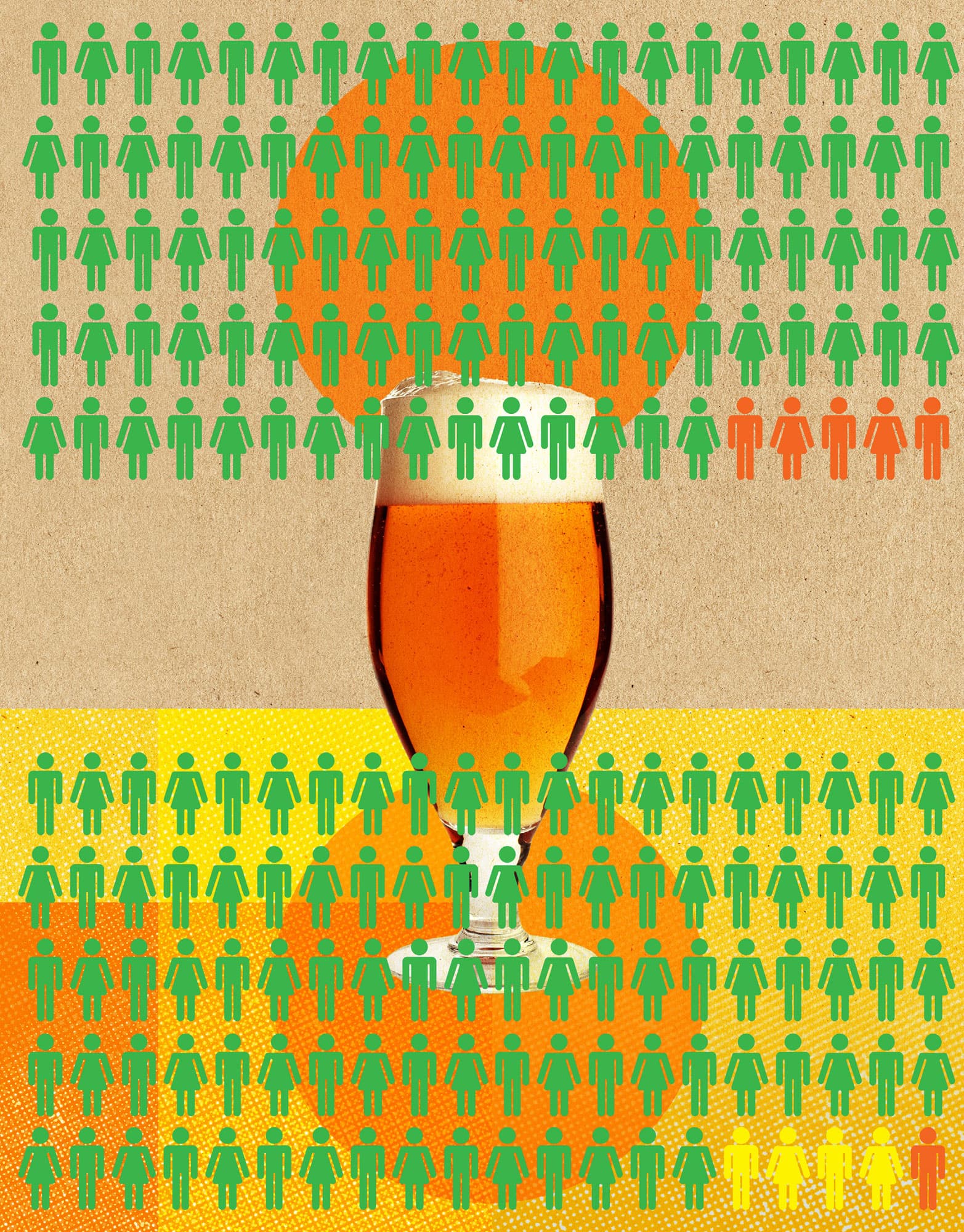
ABSOLUTE RISK
the 30-second calculation
Absolute risk is calculated using the number of times an event occurred in a group of interest divided by the total population of that group. Even though this seems fairly simple, in reality getting a good estimate for the absolute risk of a disease, for example, involves combining multiple large medical studies that were conducted on thousands of people across multiple years. Absolute risk is an effective way of describing risks because it puts the frequency of an event in the context of the overall population in which it was observed, which is usually easier to understand. This ease of understanding can increase patient agency in medical decision-making. Suppose there is a medical treatment that leads to a full recovery from a disease for five people in every 100, compared with the previous treatment, which cured one out of every 100 people. The side-effects of the new treatment can now be weighed by the knowledge that it saves an extra four in 100 people. The relative risk framing of the same statistic reports a five-times increase in efficacy for the new treatment, which might be seen as overstating its benefits when the absolute risk measure is known. Absolute risk is sometimes incorrectly presented without reference to the underlying population, which can make the corresponding risk seem misleadingly small or large.
3-SECOND COUNT
An absolute risk is an estimate of the odds of an event occurring over a specified timeframe.
3-MINUTE TOTAL
A 2018 Lancet study showed that 15–95-year olds who drink one daily alcoholic drink increased their one-year risk of an alcohol-related health problem by 0.5%. Since 914 of 100,000 people experience an alcohol-related health problem anyway (e.g. diabetes), this increase for moderate drinkers equates to four extra people per 100,000.
RELATED TOPICS
See also
3-SECOND BIOGRAPHY
DAVID SPIEGELHALTER
1953–
British statistician and Winton Professor of the Public Understanding of Risk at the University of Cambridge, widely known for helping to shape media reporting of statistics and risk information
30-SECOND TEXT
Harry Gray
Absolute risk presents the risk of an event in the context of the population observed.
RELATIVE RISK
Relative risk, also known as the risk ratio, is calculated using the ratio of absolute risks between two groups for an event. It is useful because it gives an idea of how much more or less likely one group is than the other to experience an event of interest. In medical statistics, it is used to show how much more likely an experiment group, such as people who smoke, is to experience a health-related condition compared with a control group who do not. A heavy criticism of the relative risk in reporting experimental outcomes is that it does not provide a baseline of the event’s overall prevalence in the control group. For example, a relative risk of 100, which means that the risk of the experiment group is 100 times higher than the other, seems highly meaningful. However, if the absolute risk of the control group is that the event only affects one in 1 billion people, then the absolute risk for the experiment group (even though it is 100 times higher) is still very low and could be considered negligible. Much like the misuse of absolute risks, high relative risks presented in isolation can suggest the risk is much higher than it actually is. This is particularly important to avoid in medicine because it can impact the health-related decisions that people make. Good practice in reporting is to present the relative risk next to its underlying absolute risk to give the full picture.
3-SECOND COUNT
A relative risk is an estimate of the change in risk for a certain event between two groups.
3-MINUTE TOTAL
In 2011, bacon sandwiches made headlines in the UK for allegedly increasing the risk of bowel cancer by 20% (if consumed daily). This scary statistic was widely scrutinized by risk communicators, since its overall absolute risk was an increase of just 1 (from 5 to 6) in 100 people.
RELATED TOPICS
See also
30-SECOND TEXT
Harry Gray
Relative risks can be put into perspective using data from two absolute risks.

NUMERICAL BIAS
the 30-second calculation
Numerical bias is an established concept in statistical estimation. It can have a range of different causes, such as non-random sampling or using models that are too simple, each of which can have different effects. Scientific experiments and statistical models are generally designed to minimize numerical bias, but it can easily go unnoticed. An example of numerical bias in everyday life arises in electronic timetables at bus stops. When there is no traffic, the timetable seems to do very well at estimating the arrival time of the next bus. However, when there is heavy traffic the story is different. This is because the speed of the traffic is not accounted for by the tracking system on the bus, only its current location. The arrival estimate is only accurate when there is no traffic, leading to the frustrating situation of ‘5 mins’ being shown on the timetable for much longer than a single minute. This estimate is numerically biased because it is systematically underestimating the actual time till the bus arrives during traffic. Numerical bias is not always a bad thing, though. If the bus is always 10 minutes late, then we can adjust for this by getting to the stop 9 minutes later than usual and only wait for 1 minute. However, if the bus always arrives randomly up to 10 minutes late, then we should decide to arrive on time, but could be waiting for up to 10 minutes.
3-SECOND COUNT
Numerical bias is a statistical term for when a mathematical quantity systematically differs from the actual quantity that it is intended to represent.
3-MINUTE TOTAL
Numerical bias is an important thing to be aware of when computing statistics as it leads to inaccuracies. These inaccuracies can have dramatic consequences when estimating the effectiveness of a new drug or trying to predict a political election result.
RELATED TOPICS
See also
3-SECOND BIOGRAPHY
CHARLES STEIN
1920–2016
American statistician whose work on biased estimation challenged the traditional statistical thinking that bias was always bad
30-SECOND TEXT
Harry Gray
Bus arrival times that are estimated without allowing for traffic are likely to be biased.