The Princeton Guide to Evolution

III.3

Theory of Selection in Populations

Kent E. Holsinger

OUTLINE

1. An example of natural selection

2. Fisher’s fundamental theorem of natural selection

3. Patterns of selection

4. Components of selection

5. Maintenance of polymorphism

6. Selection and other processes

7. Synthesis and conclusions

This chapter provides an introduction to the genetics of natural selection. It focuses on selection associated with differences in probability of survival determined by alternative alleles at a single locus, but it also illustrates some of the properties associated with natural selection when selection arises at other stages in the life cycle, when selection varies in space or time, when selection interacts with other evolutionary processes (like mutation, migration, and genetic drift), and when fitness depends on the genotype at more than one locus.

GLOSSARY

Absolute Viability. The probability of survival from zygote to adult.

Bateman’s Principle. In most species, females invest more heavily in offspring than males and remate less quickly, leading to greater variation in reproductive success among males than females.

Cline. A gradual change in allele frequency along a geographical transect.

Directional Selection. A mode of natural selection in which one of the homozygous genotypes has the highest fitness, the heterozygote is intermediate, and the other homozygote has the lowest fitness.

Disruptive Selection. A mode of natural selection in which the heterozygous genotype has a lower fitness than either of the the homozygous genotypes.

Equilibrium. A state of a population in which its allele frequency does not change from one generation to the next. It may be a monomorphic equilibrium in which only one allele is present, or a polymorphic equilibrium in which various evolutionary forces are precisely balanced and the allele frequency remains constant.

Fertility Selection. Natural selection associated with differences in the number of offspring produced. These differences may depend on the genotype of both male and female partners or they may be related only to differences among females, fecundity selection, or only to differences among males, virility selection.

Fitness. The probability of survival from zygote to adult. More generally, the performance of a genotype in survival and reproduction.

Fixation. A population is fixed for an allele if that allele is the only one present. The population could also be called monomorphic for that allele.

Mean Fitness. The average probability of survival from zygote to adult, calculated as the product of genotype frequency and genotype viability and summed across all genotypes.

Mode of Natural Selection. The type of natural selection as determined by which genotype has the highest fitness, which is intermediate, and which has the lowest fitness.

Monomorphic Equilibrium. An equilbrium in which only one allele is present.

Monomorphism. A population is monomorphic at a particular locus if only one allele is present in the entire population. The population could also be said to be fixed for that allele.

Overdominance. A mode of natural selection in which the fitness of heterozygotes is greater than that of homozygotes.

Polymorphic Equilibrium. An equilibrium in which more than one allele is present.

Polymorphism. A population is polymorphic at a particular locus if more than one allele is present at that locus in the population.

Relative Viability. The viability of a genotype relative to another genotype, specifically the absolute viability of one genotype divided by the absolute viability of another.

Selection Coefficient. The difference in relative fitness between a particular genotype and the genotype with a relative fitness of 1.

Stabilizing Selection. A mode of natural selection in which the heterozygous genotype has a higher fitness than either of the homozygous genotypes.

Viability Selection. Natural selection associated with differences in the probability of survival.

1. AN EXAMPLE OF NATURAL SELECTION

The basics of natural selection are easy to understand. To illustrate them we’ll use a numerical example based on data from Drosophila pseudoobscura collelcted by Theodosius Dobzhansky nearly 70 years ago. This species has chromosome inversion polymorphisms. Although the inversions contain many genes, they are inherited as if they were alternative alleles at a single Mendelian locus, so we can treat them as single-locus genotypes and study their evolutionary dynamics. We’ll be considering two inversion types: the Standard inversion type, ST, and the Chiricahua inversion type, CH.

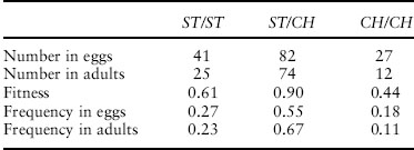
Dobzhansky counted the number of each of the three genotypes both at the egg stage and at the adult stage. He then calculated the fraction of each genotype that survived, its fitness. Data from one of his experiments are shown in table 1. As you can see, the genotypes differ in fitness. In fact, as you can also see from the table, the frequency of heterozygotes increased and the frequency of homozygotes decreased within this generation. That is not an evolutionary response, since there has been no transmission of genetic information from one generation to the next. But the differences are heritable, so the genotype frequencies will change in response to natural selection from one generation to the next.

Table 1. Data from Dobzhansky’s experiment on Drosophila pseudoobscura.

Note: The frequencies in adults do not sum to 1 because of rounding.

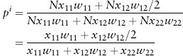
Of course, we’d like to be able to predict how these frequencies will change over time. To do that, we need to build an algebraic model that allows us to describe how genotype and allele frequencies change in response to natural selection. We will use the notation in table 2 throughout our development of this model. Notice that if we know the frequency of each genotype in eggs and the total number of eggs, we can calculate the number of individuals as the product of the number of eggs and the genotype frequency. For example, if the number of eggs is N and the frequency of the ST/ST homozygote is x₁₁, then the number of ST/ST homozygotes is Nx₁₁. If we also know the probability that each genotype will survive from egg to adult (its fitness), we can calculate the number of adults as the product of the number of zygotes and their fitnesses. For ST/ST that’s Nx₁₁w₁₁. Putting this all together, we can calculate the frequency of the ST chromosome in adults as

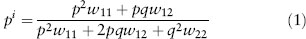
We need to assume that these differences in survival are the only differences relevant for natural selection, that no mutation or migration is occurring, and that the population is large enough that we can ignore genetic drift. That’s a lot of assumptions, but if we make them, the Hardy-Weinberg principle guarantees two things: (1) the frequency of the ST chromosomes in newly formed zygotes of the next generation will be the same as it is in adults of this generation, and (2) the genotype frequencies in those zygotes will be in Hardy-Weinberg proportions. As a result, we can make that formula a little simpler:

Table 2. Notation used to describe natural selection.

Symbol	Definition
N	total number of eggs
x₁₁	frequency of ST/ST
x₁₂	frequency of ST/CH
x₂₂	frequency of CH/CH
w₁₁	fitness of ST/SH
w₁₂	fitness of ST/CH
w₂₂	fitness of CH/CH

It probably doesn’t look like it, but we can do a lot with that formula thanks to a theorem proven by Sir Ronald Fisher.

2. FISHER’S FUNDAMENTAL THEOREM OF NATURAL SELECTION

To start, let’s take a look at the denominator of equation (1): p² is the probability that a randomly chosen egg is ST/ST and w₁₁ is the probability that it survives to adulthood, and the other two terms, 2pq and q₂, are the same probabilities for ST/CH and CH/CH, respectively. So the denominator is the probability that a randomly chosen egg survives to adulthood or, equivalently, the average probability of survival. For convenience we often refer to the probability of survival as fitness, and statisticians often use the word mean to refer to averages. So the name Fisher gave to this quantity is mean fitness, and we typically symbolize it with the symbol .

The mean fitness is a property of a population, not of any one individual in it, and it depends not only on the fitness of each genotype but also on their frequencies. So it might be more appropriate to write it as to emphasize that the mean fitness of a population depends on its allele frequency. In fact, if the genotype fitnesses remain constant, the only way the mean fitness of the population can change over time is if its allele frequencies change.

This is where Fisher’s fundamental theorem of natural selection comes in. It tells us that allele frequencies will change in response to natural selection in such a way that the mean fitness of the population increases from one generation to the next. Mathematically, we say that

with equality holding only when the allele frequency has reached a point where is at a maximum. Recall that is the average probability of survival, so another way of stating Fisher’s theorem is to say that natural selection increases adaptation in the sense that it increases the average probability of survival in the population.

3. PATTERNS OF SELECTION

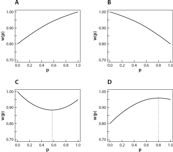
Armed with Fisher’s theorem, we’re now ready to make progress in understanding how populations will respond to natural selection. The key is to understand how the shape of depends on the mode of natural selection (figure 1). The mode of natural selection is determined by which of the three genotypes has the highest fitness, which has an intermediate fitness, and which has the lowest fitness. There are three modes of natural selection: directional selection, disruptive selection, and stabilizing selection. Throughout the discussions that follows, we’ll assume that p refers to the frequency of an allele we’ll label A₁ and that 1 – p is the frequency of the alternative allele A₂.

Figure 1. Patterns of natural selection at one locus with two alleles. (A) Directional: w₁₁ > w₁₂ > w₂₂. (B) Directional: w₁₁ < w₁₂ < w₂₂. (C) Disruptive: w₁₁ > w₁₂, w₂₂ > w₁₂. (D) Stabilizing: w₁₁ < w₁₂, w₂₂ < w₁₂. The dashed vertical lines in (C) and (D) indicate the allele frequency corresponding to a polymorphic equilibrium. There is no polymorphic equilibrium in (A) or (B).

Directional Selection

Directional selection occurs when one of the homozygotes has the highest fitness, the heterozygote has an intermediate fitness, and the other homozygote has the lowest fitness. In figure 1A the fitnesses are w₁₁ = 1.0, w₁₂ = 0.95, and w₂₂ = 0.80. In figure 1B the fitnesses are w₁₁ = 0.80, w₁₂ = 0.95, and w₂₂ = 1.0. In Figure 1A, Fisher’s theorem tells us that natural selection will cause the frequency of A₁ to increase in every generation. Only if pⁱ is greater than p, will be greater than as required by Fisher’s theorem. Moreover, the frequency of A₁ will continue increasing until it equals 1, meaning that all the alleles in the population are A₁ and that allele A₂ has been lost. Under these conditions we say that allele A₁ is fixed in the population and that the population is monomorphic. Similarly, natural selection like that in figure 1B will lead to fixation of allele A₂.

In short, directional selection will eventually cause a population to become monomorphic for the homozygous genotype with the highest fitness.

Disruptive Selection

Disruptive selection occurs when the heterozygote has a lower fitness than either of the homozygotes (figure 1C). In this case, the outcome of natural selection depends on the initial allele frequency. If the initial frequency of allele A₁ is smaller than the value of p associated with the dashed line in figure 1C, its frequency will decline from one generation to the next until the population is fixed for allele A₂. If, on the other hand, its initial frequency is larger than the value of p associated with the dashed line, its frequency will increase from one generation to the next until the population is fixed for allele A₁. If it happened that the initial frequency were exactly equal to the value of p associated with the dashed line, it wouldn’t change from one generation to the next. The population would be in equilibrium.

In this case, the equilibrium is not important biologically, because if the allele frequency departs ever so slightly from the equilibrium value, natural selection will push it farther and farther away. In short, disruptive selection will eventually cause a population to become monomorphic for one of the alleles, but which allele becomes fixed depends on the initial frequency of the allele. Two populations subject to identical disruptive selection pressures will diverge even further if their initial allele frequencies are different enough.

Stabilizing Selection

Stabilizing selection occurs when the heterozygote has a higher fitness than either of the homozygotes (figure 1D). In this case, the population always evolves to an intermediate allele frequency. If the initial frequency of allele A₁ is smaller than the value of p associated with the dashed line in figure 1D, its frequency will increase from one generation to the next until it reaches a value corresponding to that dashed line. If, on the other hand, the initial frequency of allele A₁ is larger than the value of p associated with the dashed line in figure 1D, its frequency will decrease from one generation to the next until it reaches a value corresponding to that dashed line.

Under stabilizing selection, the polymorphic equilibrium is important biologically, because even if the allele frequency happens to depart from the equilibrium value, natural selection will pull it back. Unlike the situation under directional or disruptive selection, in which natural selection acts to eliminate variation, under stabilizing selection natural selection acts to preserve it. Moreover, if two populations are subject to the same stabilizing selection pressures, they will converge on the same allele frequency no matter how different they were initially.

Returning to Our Example

If we now return to our initial example, we recognize that we have an example of stabilizing selection. The fitness of the ST/ST karyotype is 0.61, that of the ST/CH karyotype is 0.90, and that of the CH/CH karyotype is 0.44. The heterozygous karyotype is the most fit, and we therefore predict that natural selection will lead to maintenance of both inversion types in the population. We would even predict that if we start an experimental population with a low frequency of ST its frequency will increase, and that if we start with a high frequency of ST it frequency will decrease. That’s precisely what Dobzhansky’s experiments showed.

4. COMPONENTS OF SELECTION

So far we have discussed natural selection as if it happens only as a result of differences in the probability of survival, but selection can happen at any life stage, and when it does, the results can be quite different from those we have discussed so far. The specific type of natural selection we have been discussing so far is viability selection. Some other important types of selection are fertility selection, sexual selection, and gametic selection. Any one or all of these types of natural selection can influence how allele frequencies change from one generation to the next.

Fertility Selection

In its most general form, fertility selection occurs when the number of offspring produced from a mating depends on both male and female genotypes. For example, Andrew Clark and Marcus Feldman studied the number of offspring produced by Drosophila melanogaster in experimental crosses (table 3). Their results show not only that the number of offspring produced may depend on the genotypes involved, but also that the same pair of genotypes can produce different numbers of offspring depending on which genotype is male and which is female.

Table 3. The number of offspring produced by singly inseminated females of Drosophila melanogaster as a function of mating type in Clark and Feldman’s experiment (simplified for this presentation).

Note: Female genotypes are in rows; male genotypes are in columns.

For example, a cross in which ey²/+ is female and ey²/ey² is male produces 115 offspring, but one in which the genotypes are reversed produces only 61. Perhaps even more surprisingly, the number of offspring a +/+ female produces depends on whether she mates with a +/+ male (57 offspring), an ey²/+ male (74 offspring), or an ey²/ey² male (78 offspring). Even though we don’t know why these differences exist, they are reproducible, so we do know they will lead to changes in genotype and allele frequencies over time, even if the three genotypes have equal probabilities of survival.

Sexual Selection

Sexual selection occurs when genotypes differ in their probability of mating. In most species females invest more in offspring than males, and they are not able to remate as quickly as males. As a result, there is more competition for mates among males than females, and females are less likely to go unmated than males. This is known as Bateman’s principle. As a result, sexual selection often takes one of two forms: male-male competition, in which males compete for access to females, and female choice, in which females select the males with whom they will mate. In the Clark and Feldman experiment, for example, female Drosophila melanogaster preferred wild-type, +/+, males to either heterozygotes or homozygotes for ey² regardless of their own genotype.

Sexual selection favors traits that enhance the probability of attracting mates, like the enormous, colorful train on a peacock or the elaborate display in the vicinity of a male bowerbird nest. These traits may reduce the probability of survival, leading to a conflict between viability selection and sexual selection. The outcome will represent a compromise between these competing forces.

Gametic Selection

Gametic selection occurs when gametes differ in their probability of accomplishing fertilization (see chapter III.2). In flowering plants, genes expressed in pollen are likely to influence the rate at which pollen tubes grow down the style, and allelic differences in these genes may be associated with differences in fertilization probability. Similarly, in animals, many genes are expressed in sperm, and sperm competition can also cause allelic differences in those genes to be associated with differences in fertilization probability. In perhaps the most famous example of gametic selection, 90 percent or more functional sperm in heterozygotes for the t allele in house mice carry the t allele. Sperm carrying the wild-type allele are functionally inactivated by their t partner. Thus, gametic selection strongly favors the t allele.

Just as with sexual selection, however, alleles favored by gametic selection may be disfavored by selection at other stages in the life cycle. While gametic selection strongly favors the t allele in house mice, for example, homozygotes for the t allele are either inviable or male sterile. So viability selection strongly favors the wild-type allele. As with the conflict between viability selection and fertility selection, the outcome represents a compromise between the competing forces of gametic selection and viability selection (see chapter IV.7).

5. MAINTENANCE OF POLYMORPHISM

We have already seen that viability selection will maintain both alleles in a population when heterozygotes are most fit. Although this simple property is not universal when more than two alleles are present at a locus or when other forms of selection are acting, broadly speaking if heterozygotes are more fit than homozygotes, then selection will tend to maintain polymorphisms within populations. But heterozygote advantage, or overdominance, is not the only mechanism by which natural selection can maintain multiple alleles in populations.

Frequency-Dependent Selection

Our discussion of natural selection has so far assumed that the fitness of different genotypes remains constant over time. But it may be that the fitness of a genotype depends on the frequency of other genotypes in the population. For example, in many flowering plants, self-fertilization is prevented by genes that prevent pollen from germinating on the style of plants that share an allele with the pollen grain. As a result, even outcross pollen can fail to germinate if it happens to land on the stigma of a plant with which it shares an incompatibility allele. In this kind of system, rare genotypes will consistently be more successful in mating than common ones, because their pollen will rarely be deposited on an incompatible stigma. This is an example of negative frequency dependencee in which the fitness of an allele or a genotype increases as its frequency decreases. When fitnesses vary in this way, selection may maintain a large variety of different alleles within a population.

Spatial Variation

The fitnesses of genotypes can also depend on the particular place in which they are found. Plant genotypes favored in a sunny meadow, for example, may be different from those favored in a shady forest. If offspring from any individual can be dispersed among different habitats, the differences among them may lead to maintenance of genotypes that do well in each habitat, although the conditions under which spatial heterogeneity promotes polymorphism are complex.

For example, imagine a plant population growing in an area with sunny and shady habitats, and suppose that offspring from any one plant might be dispersed into either habitat. In many plant populations, the number of seeds produced is relatively independent of the number of seeds from which the population started, because only a certain amount of biomass can be produced in a given area, and the number of seeds produced is often proportional to biomass. In that case, the seed output from each habitat will not be influenced by the genotype composition within it. Under these conditions, selection will maintain polymorphism so long as different genotypes are favored in the two habitats.

But suppose that seed output from each habitat does depend on the genotype composition within it. Then selection will maintain a polymorphism only so long as the fitness of the heterozygote exceeds that of both homozygotes, where fitnesses are calculated as the average fitness within each habitat weighted by habitat frequency. When dispersal between habitats is limited, the condition that determines whether selection will maintain variation represents a compromise between these two extreme scenarios. In general, while spatial heterogeneity in selection can make it more likely that genetic variation is maintained, spatial heterogeneity alone is not sufficient to ensure that populations remain genetically variable.

Temporal Variation

With frequency-dependent selection, fitness varies over time, but it varies predictably as a function of the frequency of different genotypes or alleles. The fitness of genotypes may also vary over time because the environmental conditions change in ways unrelated to the genotype frequency. If one homozygous genotype is favored under some circumstances and the other is favored under different circumstances, the differences over time may lead to the maintenance of a polymorphism, but as with spatial variation, the conditions under which temporal variation promotes polymorphism are complex. In particular, if the fitness of heterozygotes varies more over time than the fitness of homozygotes, natural selection may eliminate genetic variation even when heterozgotes are more fit on average.

6. SELECTION AND OTHER PROCESSES

In our derivation of equation (1), we assumed that the only fitness differences relevant for natural selection were viability differences and that the viabilities remained the same over time. We’ve now seen that relaxing those assumptions makes predicting the response to selection complex. It shouldn’t come as a surprise that the interaction of selection with mutation, migration, and drift can also be quite complex.

Mutation

We’ve already seen that in the absence of mutation, directional selection will lead to fixation of the allele associated with the highest fitness. But suppose that in every generation, the deleterious allele arises anew by mutation in each generation, and so persists. The population will reach an equilibrium in which loss of the allele associated with selection will be balanced by gain of the allele through mutation.

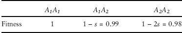
Consider the simplest case, when the deleterious allele is completely recessive, so that the relative fitnesses of the genotypes are 1, 1, and 1 – s for the homozygote for the advantageous allele, the heterozygote, and the homozygote for the deleterious allele, respectively, where s is the selection coefficient. If μ is the mutation rate from the advantageous allele to the deleterious allele, the equilibrium frequency of the deleterious allele is approximately . If the deleterious allele is only partially recessive so that the relative fitness of the heterozygote is 1 – hs, then the equilibrium frequency of the deleterious allele is approximately μ/(hs) (see chapter IV.3).

Because completely recessive alleles are “hidden” from natural selection in heterozygotes, they may occur in a much higher frequency than a partially recessive allele in which the heterozygotes have the same relative fitness (figure 2). On the other hand, because the deleterious phenotype is expressed only in recessive homozygotes, the mean fitness in a population with a pure recessive is a little higher than that in a population with a partial recessive (see chapter IV.5).

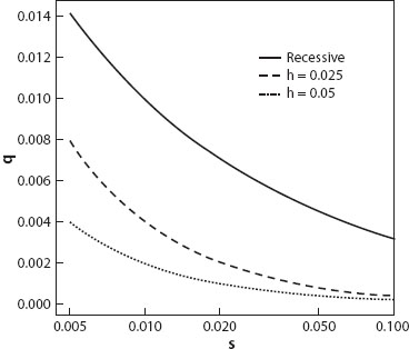
Figure 2. The equilibrium frequency of a deleterious allele with different selection coefficients and different degrees of dominance. μ = 10⁻⁶ in all cases.

Gene Flow and Migration

To most people the word migration conjures up images of birds heading south for the winter (or north for the winter in the Southern Hemisphere). To a population geneticist, the word migration means the movement of an organism from the population in which it was born to another in which it reproduces (see chapter IV.3). If a robin returns to the place where it was born to reproduce, to a population geneticist there has been no migration. Only if that robin reproduces in a place different from where it was born would a population geneticist say that migration has occurred—and the migration would be from where it was born to where it reproduced, not from where it was born to where it spent the winter. Migration is often used interchangeably with the phrase gene flow, although gene flow is sometime used to include the movement of genes into a new population founded through colonization as well as the movement of genes into an existing population.

We already learned that if the fitness of genotypes differs from one habitat to another and dispersal among habitats is limited, natural selection may lead to the maintenance of a genetic polymorphism. But suppose that the habitats, instead of being intermixed as discrete units, have a sharp boundary as you move from one part of a region to another. For example, some plant species have genotypes that are able to survive on soils with high levels of heavy metals like those found on mine tailings. These genotypes usually have lower fitness than nontolerant genotypes when growing on soil with low levels of heavy metals. In the absence of migration, we would expect all plants that grow on mine tailings to be heavy-metal tolerant and all plants that grow elsewhere to be nontolerant. But both pollen and seed move from one habitat to the other. If the area of tailings is very large, nearly every plant in the center of the tailings habitat will be a resistant genotype. As you move closer to the boundary, however, the frequency of nonresistant genotypes increases. Similarly, resistant genotypes are found out of the area of the tailings, but their frequency decreases as the distance from the mine tailings increases. The gradual change in allele frequencies along a geographical transect is referred to as a cline.

The allele frequency at any position along a cline represents a balance between natural selection favoring the genotype best suited to local circumstances and the introduction of other alleles through gene flow or migration. The width of a cline is related to the strength of selection in each habitat and the extent of dispersal between habitats. The stronger the selection, the narrower the cline, and the more the gene flow, the broader the cline.

Genetic Drift

In our discussion of natural selection so far, we’ve ignored the fact that in real populations, allele frequencies can change simply because some individuals are lucky and some are unfortunate. Some individuals may just happen to have a large number of offspring while others have few or none, and these differences may be completely unrelated to genotypic differences at the locus we happen to be studying. When such changes occur, it is referred to as genetic drift (see chapter IV.1). In large populations, we can usually ignore the influence of such random changes, but when populations are small, these types of changes can have a larger influence on the way allele frequencies change than natural selection. Although the details vary depending on the mode of selection, roughly speaking, random changes in allele frequency, genetic drift, predominate when the product of effective population size, N_e and the selection coefficient, s is less than 1. Natural selection predominates when N_es > 1. Thus, whether natural selection has an important influence on allele frequency changes depends on both the strength of the selection and the size of the population.

Table 4. A hypothetical set of relative fitnesses corresponding to directional selection for allele A₁ with s = 0.01.

Consider the set of relative fitnesses in table 4. If the effective size of the population is 50, N_es = 0.5< 1, so allele frequency changes will primarily reflect the random effects of genetic drift, even though there is strong directional selection in favor of allele A₁. If, on the other hand, the effective size of the population is 200, N_es = 2 ≫ 1, so allele frequency changes will primarily reflect the effects of natural selection and cause the frequency of A₁ to increase in every generation. When N_es<1, allelic differences are effectively neutral, meaning that even though genotypes have different fitnesses, genetic drift rather than natural selection is the predominant influence on allele frequency changes in the population.

If we could ignore genetic drift, then every advantageous mutation that arises would be guaranteed to increase in frequency as a result of natural selection. But when a new mutation arises, it is usually unique. There will be only one copy in the entire population. As a result, there’s a good chance it will be lost even if it is highly advantageous. In fact, J.B.S. Haldane showed that if the selection coefficient in favor a favorable allele is s in heterozygotes and 2s in homozygotes, the probability that it will be fixed by selection is only 2s. In other words, an allele providing a 20 percent fitness advantage to those homozygous for it has an 80 percent chance of being lost as a result of genetic drift. Most newly arisen mutations are lost, even if they are highly favorable.

7. SYNTHESIS AND CONCLUSIONS

Population geneticists have explored the genetic consequences of natural selection using mathematical models and experiments since the early 1920s, amassing a deep understanding of many complex phenomena, only a few of which have been described here. In spite of the many complexities and subtleties this work has revealed, several broad principles apply:

• Natural selection usually increases the adaptedness of individuals, making them better suited to the biotic and abiotic environments in which they exist.

• Natural selection will eliminate variation and lead to a population composed of a single genotype, if there is a single homozygous genotype that is more fit than all others. It will preserve variation, when the most fit genotype is a heterozygote. Natural selection will also eliminate variation if heterozygotes are less fit than homozygotes, but the single genotype that remains will depend on the genotype frequencies from which the population started.

• While natural selection tends to increase the level of individual adaptation, several evolutionary processes may result in compromises that reduce individual fitness. If mutation regularly introduces deleterious mutations, the frequency of the alleles will represent a balance between the mutation rate and the strength of selection. Similarly, if migration or gene flow among populations introduces genotypes that are not optimal within local populations, the fitness of individuals will be smaller than in the absence of migration.

• While differences in fitness usually lead to predictable changes in genotype frequency, in small populations, changes in allele frequency may be largely random even when genotypes differ in fitness. In particular, the chance that advantageous alleles become more common depends not only on how strongly they are favored but also on their frequency. As a result, most new mutations are lost, even if they are highly advantageous.

• Natural selection can occur simultaneously at several different life history stages: survival from zygote to reproductive adult, finding of mates, production of gametes, and production of offspring. Traits that enhance fitness at one life history stage may reduce it at another, for example, a peacock’s enormous train may enhance reproductive success of males while reducing their probability of survival.

• Corresponding with the different life history stages at which natural selection can operate are several different hierarchical levels at which it can operate: gametic, individual, and mated pair. Other chapters in this guide (see chapters III.2 and VII.9) illustrate that natural selection can even operate at the level of groups of kin and maybe even at the level of groups of unrelated individuals that share certain traits.

In short, the theory of evolution by natural selection provides a richly textured framework by which to understand an enormous diversity of evolutionary phenomena. Yet underneath all of this diversity lies Darwin’s fundamental insight: Heritable characteristics that enhance the probability of survival and reproduction will tend to become more common, and those that reduce fitness will tend to be eliminated.