
Zero-Sum Games
Zero-sum games abstract the model of combinatorial games. Fundamental examples arise naturally as LAGRANGE games from mathematical optimization problems and thus furnish an important link between game theory and mathematical optimization theory. In particular, strategic equilibria in such games correspond to optimal solutions of optimization problems. Conversely, mathematical optimization techniques are important tools for the analysis of game-theoretic situations.
As in the previous chapter, we consider games Γ with 2 agents (or players). However, we shift the viewpoint and no longer assume players taking turns in moving a system from one state into another. Instead, we assume that the players decide on strategies according to which they play the game.
More precisely, the players are assumed to have sets X and Y of possible strategies (or decisions, or actions, etc.) at their disposal. Hence a “state” of the game under this new perspective is a pair (x, y) of strategies x ∈ X and y ∈ Y.1 In fact, we consider the set
of joint strategy choices as the system underlying the game Γ, where σ0 is just an initial state, which we may attach formally to the set X × Y of joint strategies. We therefore refer to the one player as the x-player and to the other as the y-player.
Γ is a zero-sum game if there is a function

that encodes the utility of the strategic choice (x, y) in the sense that the utility values of the individual players add up to zero:
(1) u1(x, y) = U(x, y) is the gain of the x-player;
(2) u2(x, y) = –U(x, y) is the gain of the y-player.
It follows that the two players have opposing goals:
(X) The x-player wants to choose x ∈ X as to maximize U(x, y).
(Y) The y-player wants to choose y ∈ Y as to minimize U(x, y).
We denote the corresponding zero-sum game by Γ = Γ(X, Y, U).
EX. 3.1. A combinatorial game with respective strategy sets X and Y for the two players is, in principle, a zero-sum game with the utility function

EX. 3.2. The Prisoner’s dilemma is a 2-person game. However, the utilities of Ex. 1.10 do not lead to a zero-sum game.
1.Matrix games
In the case of finite strategy sets, say X = {1, . . . , m} and Y = {1, . . . , n}, a function U : X × Y → ℝ can be presented in matrix form:
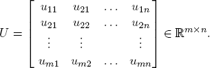
The associated matrix game is the zero-sum game Γ = (X, Y, U) where the x-player chooses a row i and the y-player a column j. This joint selection (i, j) has the utility value uij for the row player and the value (–uij) for the column player. As an example, consider the game with the utility matrix
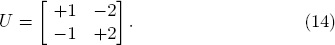
In the example (14), there is no obvious overall “optimal” choice of strategies. No matter what row i and column j are selected by the players, one of the players will find2 that the other choice would have been more profitable. In this sense, this matrix game has no “solution”.
Before pursuing this point further, we will introduce a general concept for the solution of a zero-sum game in terms of an equilibrium between both players.
2.Equilibria
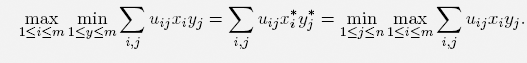
Let us assume that both players in the zero-sum game Γ = (X, Y, U) are risk avoiding and want to ensure themselves optimally against the worst case. So they consider the worst case functions
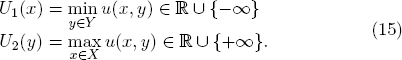
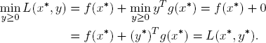
The x-player thus faces the primal problem

while the y-player is to solve the dual problem

We say that (x*, y*) ∈ X × Y is an equilibrium of the game Γ if it yields the equality
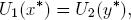
i.e., if the primal-dual inequality, in fact, attains equality:

In the equilibrium (x*, y*), none of the risk avoiding players has an incentive3 to deviate from the chosen strategy. In this sense, equilibria represent optimal strategies for risk avoiding players.
EX. 3.3. Determine the best worst-case strategies for the two players in the matrix game with the matrix U of (14) and show that the game has no equilibrium.
Give furthermore an example of a matrix game that possesses at least one equilibrium.
Finding equilibria. If the strategy sets X and Y are finite and hence the zero-sum game Γ = (X, Y, U) is a matrix game, the question whether an equilibrium exists, can — in principle — be answered in finite time by a simple procedure:
•Check each strategy pair (x*, y*) ∈ X × Y for the property (19).
If X and Y are infinite, usually the existence of equilibria can only be decided if the function U : X × Y → ℝ has special properties. From a theoretical point of view, the notion of convexity is very helpful and important.
3.Convex zero-sum games
Recall4 that a convex combination of points x1, . . . , xk ∈ ℝn is a linear combination

An important interpretation of  is based on the observation that the coefficient vector λ = (λ1 , . . . , λk) of a convex combination is a probability distribution:
•If a point xi is selected from the set {x1, . . . , xk} with probability λi, then the components of the convex combination  are exactly the expected component values of the stochastically selected point.
Another way of looking at is:
•If weights of size λi are placed on the points xi, then is their center of gravity.
A set X ⊆ ℝn is convex if X contains all convex combinations of all possible finite subsets {x1, . . . , xk} ⊆ X.
EX. 3.4. Let S = {s1, . . . , sm} be an arbitrary set with m ≥ 1 elements. Show that the set  of all probability distributions λ on S forms a compact convex subset of ℝm.
A function f : X → ℝ is convex (or convex up) if X is a convex subset of some coordinate space ℝn and for every x1, . . . , xk ∈ X and probability distribution λ = (λ1 , . . . , λk), one has

f is concave (or convex down) if g = –f is convex (up).
With this terminology, we say that the zero-sum game Γ = (X, Y, U) is convex if
| (1) | X and Y are non-empty convex strategy sets; | ||||
| (2) | the utility U : X × Y → ℝ is such that
|
The main theorem on general convex zero-sum-games guarantees the existence of at least one equilibrium in the case of compact strategy sets:
THEOREM 3.1. A convex zero-sum game Γ = (X, Y, U) with compact strategy sets X and Y and a continuous utility U admits a strategic equilibrium (x*, y*) ∈ X × Y.
Proof. Since X and Y are convex and compact sets, so is the set Z = X × Y and hence also the set Z × Z.
Consider the continuous function G : Z × Z → ℝ with the values

Since U is concave in the first variable x and (–U) concave in the second variable y, we find that G is concave in the second variable (x, y). Hence Corollary A.1 (Appendix) allows us to deduce the existence of an element (x*, y*) ∈ Z that satisfies

for all (x, y) ∈ Z and hence the inequality

This shows that x* is the best strategy for the x-player if the y-player chooses y* ∈ Y. Similarly, y* can be proved to be optimal against x*. In other words, (x*, y*) is an equilibrium of (X, Y, U).

Theorem 3.1 has important consequences not only in game theory but also in the theory of mathematical optimization in general, which we will sketch in more details in Section 4 below. To illustrate the situation, let us first look at the special case of randomizing the strategic decisions in zero-sum matrix games.
3.1.Randomized matrix games
Recall from Ex. 5.2 that a zero-sum game Γ = (X, Y, U) with finite strategy sets X and Y does not necessarily admit an equilibrium.
Suppose the players randomize the choice of their respective strategies. That is to say, the x-player decides on a probability distribution on X and chooses an i ∈ X with probability i. Similarly, the y-player chooses a probability distribution  on Y and selects j ∈ Y with probability j. Then the x-player’s expected gain is

where the uij are the coefficients of the utility matrix U.
So we arrive at a zero-sum game  where
where  is the set of probability distributions on X and
  the set of probability distributions on Y. and are compact convex sets (cf. Ex. 3.4).
Moreover, the function 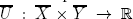 is linear, and thus continuous and both concave and convex in both components.
It follows that  is a convex game that satisfies the hypothesis of Theorem 3.1. Therefore, admits an equilibrium. This proves the VON NEUMANN’s Theorem:
THEOREM 3.2 (VON NEUMANN [32]). Let U ∈ ℝm×n be an arbitrary matrix with coefficients uij. Then there exist x* ∈ X and y* ∈ Y such that
where X is the set of all probability distributions on {1, . . . , m} and Y the set of all probability distributions on {1, . . . , n}.
3.2.Computational aspects
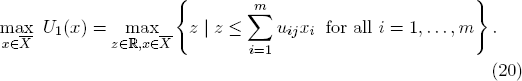
While it is generally not easy to compute equilibria in zero-sum games, the task becomes tractable for randomized matrix games. Consider, for example, the two sets X = {1, . . . , m} and Y = { 1 , . . . , n} and the utility matrix

For the probability distributions x ∈ and y ∈ , the expected utility for the x-player is

The worst case for the row player occurs when the column player selects a probability distribution that puts the full weight 1 on k ∈ Y such that
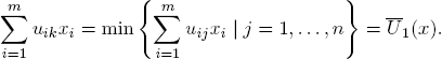
Similarly, the worst case for the column player it attained when the row player places the full probability weight 1 onto  ∈ X such that
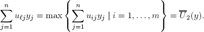
This yields

This analysis shows:
PROPOSITION 3.1. If (z*, x*) is an optimal solution of (20) and (w*, y*) and optimal solution of (21), then

REMARK 3.1. As further outlined in Section 4.5 below, the optimization problems (20) and (21) are linear programs that are dual to each other. They can be solved very efficiently in practice. For explicit solution algorithms, the interested reader may consult the standard literature on mathematical optimization.5
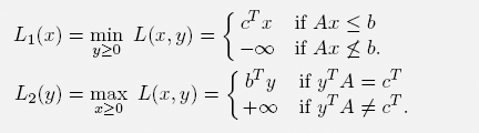
The analysis of zero-sum games is closely connected with a fundamental technique in mathematical optimization. A very general formulation of an optimization problem is

where  could be any set and f : → ℝ an arbitrary objective function. In our context, however, we will look at more concretely specified problems and understand by a mathematical optimization problem a problem of the form

where X is a nonempty subset of some coordinate space ℝn with an objective function f : X → ℝ.
The vector valued function g : X → ℝm is a restriction function and combines m real-valued restriction functions gi : X → ℝ as its components. The set of feasible solutions of (22) is

REMARK 3.2. The model (22) formulates an optimization problem as a maximization problem. Minimization problems can, of course, also be formulated within this model because of

The optimization problem (22) defines a zero-sum game Λ =  with the so-called LAGRANGE function
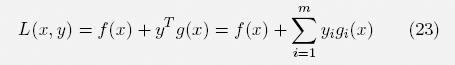
as its utility. We refer to Λ as a LAGRANGE game.6 The worst-case utility functions of the two players in Λ are:

EX. 3.5 (Convex LAGRANGE games). If X is convex and the objective function f : X → ℝ as well as the restriction functions gi : X → ℝ are concave, then the LAGRANGE game Λ = is a convex zero-sum game. Indeed, L(x, y) is concave in x for every fixed y ≥ 0 and linear in y for every fixed x ∈ X. Since linear functions are in particular convex, the game Λ is convex.
4.1.Complementary slackness
The choice of an element x ∈ X with at least one restriction violation gi(x) < 0 would allow the y-player in the LAGRANGE game Λ = to increase its utility value infinitely with the choice yi ≈ ∞. So the risk avoiding x-player will always try to select a feasible x.
On the other hand, if all of the feasibility requirements gi(x) ≥ 0 are satisfied, the best the y-player can do is the selection of y ∈  such that the so-called complementary slackness condition

is met. Consequently, one finds:
LEMMA 3.1. If (x*, y*) is an equilibrium of the LAGRANGE game Λ, then x* is an optimal solution of problem (22).
Proof. For every feasible x ∈ , y* ≥ 0 yields (y*)Tg(x) ≥ 0 and, therefore,

So x* is optimal.
4.2.The KKT-conditions
Lemma 3.1 indicates the importance of being able to identify equilibria in LAGRANGE games. In order to establish necessary conditions, i.e., conditions which candidates for equilibria must satisfy, we impose further assumptions on problem (22):
(1)X ⊆ ℝn is a convex set, i.e., X contains with every x, x′ also the whole line segment

(2)The functions f and gi in (22) have continuous partial derivatives ∂f(x)/∂xj and ∂gi(x)/∂xj for all j = 1, . . . , n.
It follows that also the partial derivatives of the LAGRANGE function L exist. So the marginal change of L into the direction d of the x-variables is

REMARK 3.3 (JACOBI matrix). The (m × n) matrix Dg(x) having as coefficients the partial derivatives

of a function g : ℝn → ℝm is known as a functional or JACOBI7 matrix. It provides a compact matrix notation for the marginal change of the Lagrange function:

LEMMA 3.2 (KKT-conditions). The pair (x, y) ∈ X × cannot be an equilibrium of the LAGRANGE game Λ unless:
(K0) g(x) ≥ 0;
(K1) yTg(x) = 0;
(K3) ∇xL(x, y)d ≤ 0 holds for all d such that x + d ∈ X.
Proof. We already know that the feasibility condition (K0) and the complementary slackness condition (K1) are necessarily satisfied by an equilibrium. If (K3) were violated and ∇xL(x, y)d > 0 were true, the x-player could improve the L-value by moving a bit into direction d. This would contradict the definition of an “equilibrium”.
REMARK 3.4. The three conditions of Lemma 3.2 are the so-called KKT-conditions.8 Although they are always necessary, they are not always sufficient to conclude that a candidate (x, y) is indeed an equilibrium.
4.3.Shadow prices
Given m functions  and m scalars b1, . . . , bm ∈ ℝ, the optimization problem

is of type (22) with the m restriction functions gi(x) = bi – ai(x) and has the LAGRANGE function

For an intuitive interpretation of the problem (26), think of the data vector
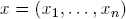
as a plan for n products to be manufactured in quantities xj and of f(x) as the market value of x.
Assume that x requires the use of m materials in quantities a1(x) , . . . , am(x) and that the parameters b1, . . . , bm describe the quantities of the materials already in the possession of the manufacturer.
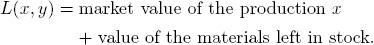
If the numbers y1, . . . , ym represent the market prices (per unit) of the m materials, we find that L(x, y) is the total value of the manufacturer’s assets:
The manufacturer would like to have that value as high as possible by deciding on an appropriate production plan x.
“The market” is an opponent of the manufacturer and looks at the value

which is the value of the materials the manufacturer must still buy on the market for the production of x minus the value of the production that the market would have to pay to the manufacturer for the production x.
The market would like to set the prices yi so that –L(x, y) is as large as possible. Hence:
•The manufacturer and the market play a LAGRANGE game Λ.
•An equilibrium (x*, y*) of Λ reflects an economic balance: Neither the manufacturer nor the market has a guaranteed way to improve their value by changing the production plan or by setting different prices.
In this sense, the production plan x* is optimal if (x*, y*) is an equilibrium. The optimal market prices  are the so-called shadow prices of the m materials.
The complementary slackness condition (K1) says that a material which is in stock but not completely used by x* has zero market value:

The condition (K2) implies that x* is a production plan of optimal value f(x*) = L(x*, y*) under the given restrictions. Moreover, one has

which says that the price of the materials used for the production x* equals the value of the inventory under the shadow prices 
Property (K3) says that the marginal change ∇xL(x*, y*)d of the manufacturer’s value L is negative in any feasible production modification from x* to x* + d and only profitable for the market because

We will return to production games in the context of cooperative game theory in Section 8.3.2.
4.4.Equilibria of convex LAGRANGE games
Remarkably, the KKT-conditions turn out to be not only necessary but also sufficient for the characterization of equilibria in convex LAGRANGE games with differentiable objective functions. This gives a way to compute such equilibria and hence to solve optimization problems of type (22) in practice9 :
•Find a solution (x*, y*) ∈ X ×  for the KKT-inequalities. (x*, y*) will yield an equilibrium in Λ =
  and x* will be an optimal solution for (22).
Indeed, one finds:
THEOREM 3.3. A pair (x*, y*) ∈ X × is an equilibrium of the convex LAGRANGE game Λ = if and only if (x*, y*) satisfies the KKT-conditions.
Proof. From Lemma 3.2, we know that the KKT-conditions are necessary. To show sufficiency, assume that (x*, y*) ∈ X × satisfies the KKT-conditions. We must demonstrate that (x*, y*) is an equilibrium of the convex LAGRANGE game Λ = , i.e., satisfies

for the function L(x, y) = f(x) + yTg(x).
Since x ↦ L(x, y*) is a concave function, we have for every x ∈ X,

Because (K2) guarantees ∇xL(x*, y*)(x – x*) ≤ 0, we conclude

which implies the first equality in (27). For the second equality, (K0) and (K1) yield g(x*) ≥ 0 and (y*)Tg(x*) = 0 and therefore:
4.5.Linear programs
A linear program (LP) in standard form is an optimization problem of the form

where c ∈ ℝn and b ∈ ℝm are parameter vectors and A ∈ ℝm×n a matrix, and thus is a mathematical optimization problem with a linear objective function f(x) = cTx and restriction function g(x) = b – Ax so that

The feasibility region of (28) is the set of all nonnegative solutions of the linear inequality system Ax ≤ b:


and yields for any x ≥ 0 and y ≥ 0:

The optimum value of L2 is found by solving the dual associated linear program

EX. 3.6. Since yTb = bTy and (cT – yTA)x = xT(c – ATy) holds, the dual linear program (29) can be formulated equivalently in standard form:

The main theorem on linear programming is:
THOREM 3.4 (Main LP-Theorem). For the LP (28) the following holds:
| (A) | An optimal solution x* exists if and only if both the LP (28) and the dual LP (29) have feasible solutions. |
| (B) | A feasible x* is an optimal solution if and only if there exists a dually feasible solution y* such that |

Proof. Assume that (28) has an optimal solution x* with value z* = cTx*. Then cTx ≤ z* holds for all feasible solutions x. So the FARKAS Lemma10 guarantees the existence of some y* ≥ 0 such that

Noticing that y* is dually feasible and that L1(x*) ≤ L2(y) holds for all y ≥ 0, we conclude that y* is, in fact, an optimal dual solution:

This argument establishes property (B) and shows that the existence of an optimal solution necessitates the existence of a dually feasible solution. Assuming that (28) has at least one feasible solution x, it therefore remains to show that the existence a dual feasible solution y implies the existence of an optimal solution.
To see this, note first

So each dually feasible y satisfies –bTy ≤ −w*. Applying now the FARKAS Lemma to the dual linear program in the form (30), we find that a parameter vector x* ≥ 0 exists with the property

On the other hand, the primal-dual inequality yields L1(x*) ≤ w*. So x* must be an optimal feasible solution.
General linear programs. In general, a linear program refers to the problem of optimizing a linear objective function over a polyhedron, namely the set of solutions of a finite system of linear equalities and inequalities and, therefore, can be formulated as

with coefficient vectors c ∈ ℝn, b ∈ ℝm, d ∈ ℝk and matrices A ∈ ℝm×n and B ∈ ℝk×n.
If no equalities occur in the formulation (31), one has as a linear program in canonical form:

Because of the equivalence

the optimization problem (31) can be presented in canonical form:

Moreover, since any vector x ∈ ℝn can be expressed as the difference
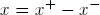
of two (nonnegative) vectors  one sees that each linear program in canonical form is equivalent to a linear program in standard form:

The LAGRANGE function of the canonical form is the same as for the standard form. Since the domain of L1 is now X = ℝn, the utility function L2(y) differs accordingly:
Relative to the canonical form, the optimum value of L2 is found by solving the linear program

Nevertheless, it is straightforward to check that Theorem 3.4 is literally valid also for a linear program in its canonical form.
Linear programming problems are particularly important in applications because they can be solved efficiently. In the theory of cooperative games with possibly more than two players (see Chapter 8), linear programming is a structurally analytical tool. We do not go into algorithmic details here but refer to the standard mathematical optimization literature.11
4.6.Linear programming games
A linear programming game is a LAGRANGE game that arises from a linear program. If c ∈ ℝn, b ∈ ℝm and A ∈ ℝm×n are the problem parameters, we may denote is by

where

is the underlying LAGRANGE function. Linear programming games are convex. In particular, Theorem 3.4 implies:
(1)A linear programming game admits an equilibrium if and only if the underlying linear program has an optimal solution.
(2)The equilibria of a linear programming game are precisely the pairs (x*, y*) of primally and dually optimal solutions.
EX. 3.7. Show that every randomized matrix game is a linear programming game. (See Section 3.3.2.)
_____________________________
1As in the Prisoner’s dilemma (Ex. 1.10).
2In hindsight!
3In hindsight.
4See also Appendix A.2 for more details.
6The idea goes back to J.-L. LAGRANGE (1736-1813).
7C.G. JACOBI (1804-1851).
8Named after the mathematicians KARUSH, KUHN and TUCKER.
9It is not the current purpose to investigate further computational aspects in details, which can be found in the established literature on mathematical programming.
10See Lemma A.6 in the Appendix.

