Linear Mappings and Matrices

6.1 Introduction

Consider a basis S = {u₁, u₂,..., u_n} of a vector space V over a field K. For any vector υ 2 V, suppose υ = a₁ u₁ + a₂ u₂ + … + a_n u_n

Then the coordinate vector of υ relative to the basis S, which we assume to be a column vector (unless otherwise stated or implied), is denoted and defined by

Recall (Section 4.11) that the mapping υ 7![υ _S, determined by the basis S, is an isomorphism between V and Kⁿ.

This chapter shows that there is also an isomorphism, determined by the basis S, between the algebra A (V)of linear operators on V and the algebra M of n-square matrices over K. Thus, every linear mapping F: V → V will correspond to an n-square matrix [F]_S determined by the basis S. We will also show how our matrix representation changes when we choose another basis.

6.2 Matrix Representation of a Linear Operator

Let T be a linear operator (transformation) from a vector space V into itself, and suppose S = {u₁, u₂,..., u_n} is a basis of V. Now T (u₁), T (u₂),…, T (u_n) are vectors in V, and so each is a linear combination of the vectors in the basis S; say,

The following definition applies.

DEFINITION:   The transpose of the above matrix of coefficients, denoted by m_S (T) or [T _S, is called the matrix representation of T relative to the basis S, or simply the matrix of T in the basis S. (The subscript S may be omitted if the basis S is understood.)

Using the coordinate (column) vector notation, the matrix representation of T may be written in the form

That is, the columns of m (T) are the coordinate vectors of T (u₁), T (u₂),…, T (u_n), respectively.

EXAMPLE 6.1   Let F: R ² → R ² be the linear operator defined by F (x, y) = (2x + 3 y, 4 x 5y).

(a) Find the matrix representation of F relative to the basis S = {u₁, u₂} = {(1, 2), (2, 5)}.

(1) First find F (u₁), and then write it as a linear combination of the basis vectors u₁ and u₂. (For notational convenience, we use column vectors.) We have

Solve the system to obtain x = 52, y = 22. Hence, F(u₁) = 52 u₁ − 22u₂.

(2) Next find F(u₂), and then write it as a linear combination of u₁ and u₂:

Solve the system to get x = 129, y = −55. Thus, F (u₂) = 129 u₁ 55 u₂.

Now write the coordinates of F (u₁) and F (u₂) as columns to obtain the matrix

(b) Find the matrix representation of F relative to the (usual) basis E = {e₁, e₂} = {(1, 0), (0, 1)}.

Find F (e₁) and write it as a linear combination of the usual basis vectors e₁ and e₂, and then find F (e₂) and write it as a linear combination of e₁ and e₂. We have

Note that the coordinates of F (e₁) and F (e₂) form the columns, not the rows, of [F _E. Also, note that the arithmetic is much simpler using the usual basis of R ².

EXAMPLE 6.2   Let V be the vector space of functions with basis S = {sin t, cos t, e^3t}, and let D : V → V be the differential operator defined by D (f (t)) = d(f (t))/dt. We compute the matrix representing D in the basis S:

and so

Note that the coordinates of D (sin t), D (cos t), D (e^3t) form the columns, not the rows, of [D].

Matrix Mappings and Their Matrix Representation

Consider the following matrix A, which may be viewed as a linear operator on R², and basis S of R²:

(We write vectors as columns, because our map is a matrix.) We find the matrix representation of A relative to the basis S.

(1) First we write A (u₁) as a linear combination of u₁ and u₂. We have

Solving the system yields x = 7, y = 4. Thus, A(u₁) = 7 u₁ 4u₂.

(2) Next we write A (u₂) as a linear combination of u₁ and u₂. We have

Solving the system yields x = 14, y = −9. Thus, A (u₂) = 14 u₁ 9 u₂. Writing the coordinates of A (u₁)and A (u₂) as columns gives us the following matrix representation of A:

Remark: Suppose we want to find the matrix representation of A relative to the usual basis E = {e₁, e₂} = {[1, 0]^T, [0, 1^T} of R²: We have

Note that [A]_E is the original matrix A. This result is true in general:

Algorithm for Finding Matrix Representations

Next follows an algorithm for finding matrix representations. The first Step 0 is optional. It may be useful to use it in Step 1 (b), which is repeated for each basis vector.

ALGORITHM 6.1:   The input is a linear operator T on a vector space V and a basis S = {u₁, u₂,..., u_n} of V. The output is the matrix representation [T]_S.

Step 0.   Find a formula for the coordinates of an arbitrary vector υ relative to the basis S.

Step 1.   Repeat for each basis vector u_k in S:

(a) Find T (u_k).

(b) Write T (u_k) as a linear combination of the basis vectors u₁, u₂,..., u_n.

Step 2.   Form the matrix [T]_S whose columns are the coordinate vectors in Step 1 (b).

EXAMPLE 6.3 Let F: R ² → R² be defined by F (x, y) = (2x + 3 y, 4x − 5 y). Find the matrix representation [F]_S of F relative to the basis S = {u₁, u₂} = {(1, 2), (2, 5)}.

(Step 0) First find the coordinates of (a, b) ∈ R² relative to the basis S. We have

Solving for x and y in terms of a and b yields x = 5a + 2b, y = 2 a b. Thus,

(Step 1) Now we find F(u₁) and write it as a linear combination of u₁ and u₂ using the above formula for (a; b), and then we repeat the process for F(u₂). We have

(Step 2) Finally, we write the coordinates of F(u₁) and F (u₂) as columns to obtain the required matrix:

Properties of Matrix Representations

This subsection gives the main properties of the matrix representations of linear operators T on a vector space V. We emphasize that we are always given a particular basis S of V.

Our first theorem, proved in Problem 6.9, tells us that the “action” of a linear operator T on a vector υ is preserved by its matrix representation.

THEOREM 6.1:   Let T: V → V be a linear operator, and let S be a (finite) basis of V. Then, for any vector υ in V, [T]_S[υ]_S = [T(υ)]_S.

EXAMPLE 6.4   Consider the linear operator F on R² and the basis S of Example 6.3; that is,

Let

Using the formula from Example 6.3, we get

We verify Theorem 6.1 for this vector υ (where [F] is obtained from Example 6.3):

Given a basis S of a vector space V, we have associated a matrix [T to each linear operator T in the algebra A (V) of linear operators on V. Theorem 6.1 tells us that the “action” of an individual linear operator T is preserved by this representation. The next two theorems (proved in Problems 6.10 and 6.11) tell us that the three basic operations in A (V) with these operators—namely (i) addition, (ii) scalar multiplication, and (iii) composition—are also preserved.

THEOREM 6.2:   Let V be an n-dimensional vector space over K, let S be a basis of V, and let M be the algebra of n n matrices over K. Then the mapping

is a vector space isomorphism. That is, for any F, G ∈ A (V) and any k ∈ K,

(i) m (F + G) = m (F)+ m (G) or [F + G = [F +[G

(ii) m (kF) = km (F) or [kF = k[F

(iii) m is bijective (one-to-one and onto).

THEOREM 6.3:   For any linear operators F, G ∈ A (V),

(Here G ° F denotes the composition of the maps G and F.)

6.3 Change of Basis

Let V be an n-dimensional vector space over a field K. We have shown that once we have selected a basis S of V, every vector υ ∈ V can be represented by means of an n-tuple [υ]_S in Kⁿ, and every linear operator T in A (V) can be represented by an n n matrix over K. We ask the following natural question:

In order to answer this question, we first need a definition.

DEFINITION:   Let S = {u₁, u₂,..., u_n} be a basis of a vector space V, and let S′ = fυ₁, υ ₂,..., υ _ng be another basis. (For reference, we will call S the “old” basis and S′ the “new” basis.) Because S is a basis, each vector in the “new” basis S′ can be written uniquely as a linear combination of the vectors in S; say,

Let P be the transpose of the above matrix of coefficients; that is, let P = [p_ij],where p_ij = a_ji. Then P is called the change-of-basis matrix (or transition matrix) from the “old” basis S to the “new” basis S′.

The following remarks are in order.

Remark 1: The above change-of-basis matrix P may also be viewed as the matrix whose columns are, respectively, the coordinate column vectors of the “new” basis vectors υ_i relative to the “old” basis S; namely,

Remark 2: Analogously, there is a change-of-basis matrix Q from the “new” basis S′ to the “old” basis S. Similarly, Q may be viewed as the matrix whose columns are, respectively, the coordinate column vectors of the “old” basis vectors u_i relative to the “new” basis S′; namely,

Remark 3: Because the vectors υ ₁, υ ₂,..., υ _n in the new basis S′ are linearly independent, the matrix P is invertible (Problem 6.18). Similarly, Q is invertible. In fact, we have the following proposition (proved in Problem 6.18).

PROPOSITION 6.4:   Let P and Q be the above change-of-basis matrices. Then Q = P^-1.

Now suppose S = {u₁, u₂,..., u_n} is a basis of a vector space V, and suppose P = [p_ij is any nonsingular matrix. Then the n vectors

corresponding to the columns of P, are linearly independent [Problem 6.21 (a)]. Thus, they form another basis S′ of V. Moreover, P will be the change-of-basis matrix from S to the new basis S′.

EXAMPLE 6.5   Consider the following two bases of R²:

(a) Find the change-of-basis matrix P from S to the “new” basis S′.

Write each of the new basis vectors of S′ as a linear combination of the original basis vectors u₁ and u₂ of S. We have

Thus,

Note that the coordinates of υ ₁ and υ ₂ are the columns, not rows, of the change-of-basis matrix P.

(b) Find the change-of-basis matrix Q from the “new” basis S′ back to the “old” basis S.

Here we write each of the “old” basis vectors u₁ and u₂ of S′ as a linear combination of the “new” basis vectors υ ₁ and υ ₂ of S′. This yields

As expected from Proposition 6.4, Q = P⁻¹. (In fact, we could have obtained Q by simply finding P⁻¹.)

EXAMPLE 6.6   Consider the following two bases of R³:

and

(a) Find the change-of-basis matrix P from the basis E to the basis S.

Because E is the usual basis, we can immediately write each basis element of S as a linear combination of the basis elements of E. Specifically,

Again, the coordinates of u₁, u₂, u₃ appear as the columns in P. Observe that P is simply the matrix whose columns are the basis vectors of S. This is true only because the original basis was the usual basis E.

(b) Find the change-of-basis matrix Q from the basis S to the basis E.

The definition of the change-of-basis matrix Q tells us to write each of the (usual) basis vectors in E as a linear combination of the basis elements of S. This yields

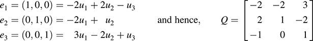
We emphasize that to find Q, we need to solve three 3 × 3 systems of linear equations—one 3 × 3 system for each of e₁, e₂, e₃.

Alternatively, we can find Q = P¹ by forming the matrix M = [P, I] and row reducing M to row canonical form:

thus,

(Here we have used the fact that Q is the inverse of P.)

The result in Example 6.6 (a) is true in general. We state this result formally, because it occurs often.

PROPOSITION 6.5:   The change-of-basis matrix from the usual basis E of Kⁿ to any basis S of Kⁿ is the matrix P whose columns are, respectively, the basis vectors of S.

Applications of Change-of-Basis Matrix

First we show how a change of basis affects the coordinates of a vector in a vector space V. The following theorem is proved in Problem 6.22.

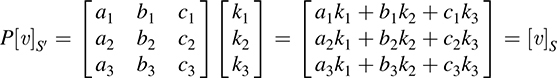
THEOREM 6.6: Let P be the change-of-basis matrix from a basis S to a basis S′ in a vector space V. Then, for any vector υ 2 V, we have

Namely, if we multiply the coordinates of υ in the original basis S by P^-1, we get the coordinates of υ in the new basis S′.

Remark 1: Although P is called the change-of-basis matrix from the old basis S to the new basis S′, we emphasize that P^-1 transforms the coordinates of υ in the original basis S into the coordinates of υ in the new basis S′.

Remark 2: Because of the above theorem, many texts call Q = P^-1, not P, the transition matrix from the old basis S to the new basis S′. Some texts also refer to Q as the change-of-coordinates matrix.

We now give the proof of the above theorem for the special case that dim V = 3. Suppose P is the change-of-basis matrix from the basis S = {u₁, u₂, u₃g to the basis S′ = fυ₁, υ ₂, υ ₃g; say,

Now suppose υ ∈ V and, say, υ = k₁υ₁ + k₂υ₂ + k₃υ₃. Then, substituting for υ ₁, υ ₂, υ ₃ from above, we obtain

Thus,

Accordingly,

Finally, multiplying the equation [υ _S = P[υ _S, by P^-1, we get

The next theorem (proved in Problem 6.26) shows how a change of basis affects the matrix representation of a linear operator.

THEOREM 6.7:   Let P be the change-of-basis matrix from a basis S to a basis S′ in a vector space V. Then, for any linear operator T on V,

That is, if A and B are the matrix representations of T relative, respectively, to S and S′, then

EXAMPLE 6.7   Consider the following two bases of R³:

and

The change-of-basis matrix P from E to S and its inverse P^-1 were obtained in Example 6.6.

(a) Write υ = (1, 3, 5) as a linear combination of u₁, u₂, u₃, or, equivalently, find [υ _S.

One way to do this is to directly solve the vector equation υ = xu₁ + yu₂ + zu₃; that is,

The solution is x = 7, y = 5, z = 4, so υ = 7 u₁ 5 u₂ + 4 u₃.

On the other hand, we know that [υ_E = [1, 3, 5]^T, because E is the usual basis, and we already know P^-1.

Therefore, by Theorem 6.6,

Thus, again, υ = 7 u₁ 5 u₂ + 4 u₃.

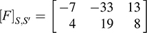
(b) Let , which may be viewed as a linear operator on R³. Find the matrix B that represents A relative to the basis S.

The definition of the matrix representation of A relative to the basis S tells us to write each of A (u₁), A (u₂), A (u₃)as a linear combination of the basis vectors u₁, u₂, u₃ of S. This yields

We emphasize that to find B, we need to solve three 3 × 3 systems of linear equations—one 3 × 3 system for each of A (u₁), A (u₂), A (u₃).

On the other hand, because we know P and P^-1, we can use Theorem 6.7. That is,

This, as expected, gives the same result.

6.4 Similarity

Suppose A and B are square matrices for which there exists an invertible matrix P such that B = P^-1 AP; then B is said to be similar to A,or B is said to be obtained from A by a similarity transformation. We show (Problem 6.29) that similarity of matrices is an equivalence relation.

By Theorem 6.7 and the above remark, we have the following basic result.

THEOREM 6.8:   Two matrices represent the same linear operator if and only if the matrices are similar.

That is, all the matrix representations of a linear operator T form an equivalence class of similar matrices.

A linear operator T is said to be diagonalizable if there exists a basis S of V such that T is represented by a diagonal matrix; the basis S is then said to diagonalize T. The preceding theorem gives us the following result.

THEOREM 6.9: Let A be the matrix representation of a linear operator T. Then T is diagonalizable if and only if there exists an invertible matrix P such that P^-1 AP is a diagonal matrix.

That is, T is diagonalizable if and only if its matrix representation can be diagonalized by a similarity transformation.

We emphasize that not every operator is diagonalizable. However, we will show (Chapter 10) that every linear operator can be represented by certain “standard” matrices called its normal or canonical forms. Such a discussion will require some theory of fields, polynomials, and determinants.

Functions and Similar Matrices

Suppose f is a function on square matrices that assigns the same value to similar matrices; that is, f (A) = f (B)whenever A is similar to B. Then f induces a function, also denoted by f, on linear operators T in the following natural way. We define

where S is any basis. By Theorem 6.8, the function is well defined.

The determinant (Chapter 8) is perhaps the most important example of such a function. The trace (Section 2.7) is another important example of such a function.

EXAMPLE 6.8   Consider the following linear operator F and bases E and S of R ²:

By Example 6.1, the matrix representations of F relative to the bases E and S are, respectively,

Using matrix A, we have

(i) Determinant of F = det (A) = 10 12 = 22;

(ii) Trace of F = tr (A) = 2 − 5 = −3.

On the other hand, using matrix B, we have

(i) Determinant of F = det (B) = 2860 + 2838 = 22;

(ii) Trace of F = tr (B) = 52 55 = 3.

As expected, both matrices yield the same result.

6.5 Matrices and General Linear Mappings

Last, we consider the general case of linear mappings from one vector space into another. Suppose V and U are vector spaces over the same field K and, say, dim V = m and dim U = n. Furthermore, suppose

are arbitrary but fixed bases, respectively, of V and U.

Suppose F: V → U is a linear mapping. Then the vectors F (υ₁), F (υ₂),..., F (υ_m) belong to U, and so each is a linear combination of the basis vectors in S′; say,

DEFINITION:   The transpose of the above matrix of coefficients, denoted by m_S;S0 (F) or [F _S;S₀, is called the matrix representation of F relative to the bases S and S′. [We will use the simple notation m (F) and [F when the bases are understood.]

The following theorem is analogous to Theorem 6.1 for linear operators (Problem 6.67).

THEOREM 6.10:   For any vector υ 2 V, [F _S;S[υ]_S = [F (υ)_S0.

That is, multiplying the coordinates of υ in the basis S of V by [F, we obtain the coordinates of F (υ) in the basis S′ of U.

Recall that for any vector spaces V and U, the collection of all linear mappings from V into U is a vector space and is denoted by Hom (V, U). The following theorem is analogous to Theorem 6.2 for linear operators, where now we let M = M _m;n denote the vector space of all m × n matrices (Problem 6.67).

THEOREM 6.11:   The mapping m: Hom (V, U) → M defined by m (F)= [F is a vector space isomorphism. That is, for any F, G ∈ Hom (V, U) and any scalar k,

(i)m (F + G) = m (F)+ m (G) or [F + G = [F +[G

(ii) m (kF) = km (F) or [kF = k[F

(iii) m is bijective (one-to-one and onto).

Our next theorem is analogous to Theorem 6.3 for linear operators (Problem 6.67).

THEOREM 6.12:   Let S, S′, S^" be bases of vector spaces V, U, W, respectively. Let F: V → U and G ∘ U → W be linear mappings. Then

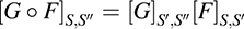
That is, relative to the appropriate bases, the matrix representation of the composition of two mappings is the matrix product of the matrix representations of the individual mappings.

Next we show how the matrix representation of a linear mapping F: V → U is affected when new bases are selected (Problem 6.67).

THEOREM 6.13: Let P be the change-of-basis matrix from a basis e to a basis e′ in V, and let Q be the change-of-basis matrix from a basis f to a basis f⁰ in U. Then, for any linear map F: V → U,

In other words, if A is the matrix representation of a linear mapping F relative to the bases e and f, and B is the matrix representation of F relative to the bases e′ and f^', then

Our last theorem, proved in Problem 6.36, shows that any linear mapping from one vector space V into another vector space U can be represented by a very simple matrix. We note that this theorem is analogous to Theorem 3.18 for m × n matrices.

THEOREM 6.14:   Let F: V → U be linear and, say, rank (F) = r. Then there exist bases of V and U such that the matrix representation of F has the form

where I_r is the r-square identity matrix.

The above matrix A is called the normal or canonical form of the linear map F.

SOLVED PROBLEMS

Matrix Representation of Linear Operators

6.1.   Consider the linear mapping F: R ² → R ² defined by F (x, y) = (3x + 4 y, 2x 5y) and the following bases of R²:

(a) Find the matrix A representing F relative to the basis E.

(b) Find the matrix B representing F relative to the basis S.

(a) Because E is the usual basis, the rows of A are simply the coefficients in the components of F (x, y); that is, using (a, b) = ae₁ + be₂, we have

Note that the coefficients of the basis vectors are written as columns in the matrix representation.

(b) First find F (u₁) and write it as a linear combination of the basis vectors u₁ and u₂. We have

Solve the system to obtain x = −49, y = 30. Therefore,

Next find F (u₂) and write it as a linear combination of the basis vectors u₁ and u₂. We have

Solve for x and y to obtain x = −76, y = 47. Hence,

Write the coefficients of u₁ and u₂ as columns to obtain

(b′) Alternatively, one can first find the coordinates of an arbitrary vector (a, b) in R² relative to the basis S.

We have

Solve for x and y in terms of a and b to get x = −3 a + 2 b, y = 2a − b. Thus,

Then use the formula for (a; b) to find the coordinates of F(u₁) and F(u₂) relative to S:

6.2.   Consider the following linear operator G on R ² and basis S:

(a) Find the matrix representation [G _S of G relative to S.

(b) Verify [G _S[υ _S = [G (υ)_S for the vector υ = (4, 3) in R².

First find the coordinates of an arbitrary vector υ = (a, b) in R² relative to the basis S.

We have

Solve for x and y in terms of a and b to get x = −5a + 2b, y = 3a − b. Thus,

(a) Using the formula for (a, b) and G (x, y) = (2 x 7 y, 4 x + 3 y), we have

(We emphasize that the coefficients of u₁ and u₂ are written as columns, not rows, in the matrix representation.)

(b) Use the formula (a, b) = (−5a + 2b)u₁ +(3a − b) u₂ to get

Then

Accordingly,

(This is expected from Theorem 6.1.)

6.3.   Consider the following 2 × 2 matrix A and basis S of R²:

The matrix A defines a linear operator on R². Find the matrix B that represents the mapping A relative to the basis S.

First find the coordinates of an arbitrary vector (a, b)^T with respect to the basis S. We have

Solve for x and y in terms of a and b to obtain x = 7 a + 3 b, y = 2 a b. Thus,

Then use the formula for (a, b)^T to find the coordinates of Au₁ and Au₂ relative to the basis S:

Writing the coordinates as columns yields

6.4.   Find the matrix representation of each of the following linear operators F on R³ relative to the usual basis E = {e₁, e₂, e₃} of R³; that is, find [F] = [F]_E:

(a) F defined by F (x, y, z) = (x + 2y −3 z, 4x − 5y 6z, 7x + 8y + 9z).

(b) F defined by the 3 × 3 matrix

(c) F defined by F (e₁) = (1, 3, 5), F (e₂) = (2, 4, 6), F (e₃) = (7, 7, 7). (Theorem 5.2 states that a linear map is completely defined by its action on the vectors in a basis.)

(a) Because E is the usual basis, simply write the coefficients of the components of F (x, y, z) as rows:

(b) Because E is the usual basis, [F] = A, the matrix A itself.

(c) Here

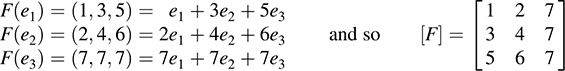
That is, the columns of [F] are the images of the usual basis vectors.

6.5. Let G be the linear operator on R³ defined by G (x, y, z) = (2 y + z, x 4 y, 3 x).

(a) Find the matrix representation of G relative to the basis

(b) Verify that [G [υ = [G (υ) for any vector υ in R³.

First find the coordinates of an arbitrary vector (a, b, c) ∈ R³ with respect to the basis S. Write (a, b, c) as a linear combination of w₁, w₂, w₃ using unknown scalars x, y, and z:

Set corresponding components equal to each other to obtain the system of equations

Solve the system for x, y, z in terms of a, b, c to find x = c, y = b c, z = a b. Thus,

(a) Because G (x, y, z) = (2y + z, x 4y, 3 x),

Write the coordinates G(w₁), G (w₂), G (w₃) as columns to get

(b) Write G (υ) as a linear combination of w₁, w₂, w₃, where υ = (a, b, c) is an arbitrary vector in R³,

or equivalently,

Accordingly,

6.6.   Consider the following 3 × 3 matrix A and basis S of R ³:

The matrix A defines a linear operator on R ³. Find the matrix B that represents the mapping A relative to the basis S. (Recall that A represents itself relative to the usual basis of R ³.)

First find the coordinates of an arbitrary vector (a, b, c) in R³ with respect to the basis S. We have

Solve for x, y, z in terms of a, b, c to get

thus,

Then use the formula for (a, b, c)^T to find the coordinates of Au₁, Au₂, Au₃ relative to the basis S:

6.7.   For each of the following linear transformations (operators) L on R ², find the matrix A that represents L (relative to the usual basis of R ²):

(a) L is defined by L (1, 0) = (2, 4) and L (0, 1) = (5, 8).

(b) L is the rotation in R ² counterclockwise by 90°.

(c) L is the reflection in R ² about the line y = x.

(a) Because {(1, 0), (0, 1)} is the usual basis of R², write their images under L as columns to get

(b) Under the rotation L, we have L (1, 0) = (0, 1) and L (0, 1) = (1, 0). Thus,

(c) Under the reflection L, we have L (1, 0) = (0, −1) and L (0, 1) = (−1, 0). Thus,

6.8.   The set S = {e^3t, te^3t, t² e^3t} is a basis of a vector space V of functions f : R → R. Let D be the differential operator on V; that is, D (f) = df = dt. Find the matrix representation of D relative to the basis S.

Find the image of each basis function:

6.9.   Prove Theorem 6.1: Let T: V ! V be a linear operator, and let S be a (finite) basis of V. Then, for any vector υ in V, [T _S[υ _S = [T (υ)_S.

Suppose S = {u₁, u₂,..., u_n}, and suppose, for i = 1,..., n,

Then [T]_S is the n-square matrix whose jth row is

Now suppose

Writing a column vector as the transpose of a row vector, we have

Furthermore, using the linearity of T,

Thus, [T (υ)_S is the column vector whose jth entry is

On the other hand, the jth entry of [T]_S[υ] _S is obtained by multiplying the jth row of [T _S by [υ _S—that is (1) by (2). But the product of (1) and (2) is (3). Hence, [T _S[υ _S and [T (υ)_S have the same entries. Thus, [T _S[υ] _S = [T (υ)_S .

6.10.   Prove Theorem 6.2: Let S = {u₁, u₂,..., u_ng be a basis for V over K, and let M be the algebra of n-square matrices over K. Then the mapping m: A (V) → M defined by m (T) = [T]_S is a vector space isomorphism. That is, for any F, G ∈ A (V) and any k 2 K, we have

(i) [F + G = [F +[G],

(ii) [kF = k[F],

(iii) m is one-to-one and onto.

(i) Suppose, for i = 1,..., n,

Consider the matrices A = [a_ij] and B = [b_ij]. Then [F] = A^T and [G] = B^T. We have, for i = 1,..., n,

Because A + B is the matrix (a_ij + b_ij), we have

(ii) Also, for i = 1,..., n,

Because kA is the matrix (ka_ij), we have

(iii) Finally, m is one-to-one, because a linear mapping is completely determined by its values on a basis. Also, m is onto, because matrix A = [a_ij in M is the image of the linear operator,

Thus, the theorem is proved.

6.11.   Prove Theorem 6.3: For any linear operators G, F ∈ A (V), [G F = [G [F].

Using the notation in Problem 6.10, we have

Recall that AB is the matrix AB = [c_ik, where . Accordingly,

The theorem is proved.

6.12.   Let A be the matrix representation of a linear operator T. Prove that, for any polynomial f (t), we have that f (A) is the matrix representation of f (T). [Thus, f (T) = 0 if and only if f (A) = 0.]

Let φ be the mapping that sends an operator T into its matrix representation A. We need to prove that φ (f (T)) = f (A). Suppose f (t) = a_n tⁿ + + a₁ t + a₀. The proof is by induction on n, the degree of f (t). Suppose n = 0. Recall that φ (I′) = I, where I′ is the identity mapping and I is the identity matrix. Thus,

and so the theorem holds for n = 0.

Now assume the theorem holds for polynomials of degree less than n. Then, because φ is an algebra isomorphism,

and the theorem is proved.

Change of Basis

The coordinate vector [υ _S] in this section will always denote a column vector; that is,

6.13.   Consider the following bases of R²:

(a) Find the change-of-basis matrix P from the usual basis E to S.

(b) Find the change-of-basis matrix Q from S back to E.

(c) Find the coordinate vector [υ of υ = (5, 3) relative to S.

(a) Because E is the usual basis, simply write the basis vectors in S as columns:

(b) Method 1. Use the definition of the change-of-basis matrix. That is, express each vector in E as a linear combination of the vectors in S. We do this by first finding the coordinates of an arbitrary vector υ = (a, b)relative to S. We have

Solve for x and y to obtain x = 4a b, y = 3 a + b. Thus,

Using the above formula for [υ]_S and writing the coordinates of the ei as columns yields

Method 2. Because Q = P^-1, find P^-1, say by using the formula for the inverse of a 2 × 2 matrix.

Thus,

(c) Method 1. Write υ as a linear combination of the vectors in S, say by using the above formula for υ = (a, b). We have υ = (5, 3) = 23u₁ − 18 u₂, and so [υ]_S = [23, −18]^T.

Method 2. Use, from Theorem 6.6, the fact that [υ]_S = P ^-1[v] _E and the fact that [υ]_E = [5, −3]^T:

6.14.   The vectors u₁ = (1, 2, 0), u₂ = (1, 3, 2), u₃ = (0, 1, 3) form a basis S of R ³. Find

(a) The change-of-basis matrix P from the usual basis E = {e₁, e₂, e₃} to S.

(b) The change-of-basis matrix Q from S back to E.

(a) Because E is the usual basis, simply write the basis vectors of S as columns:

(b) Method 1. Express each basis vector of E as a linear combination of the basis vectors of S by first finding the coordinates of an arbitrary vector υ = (a, b, c) relative to the basis S. We have

Solve for x, y, z to get x = 7a − 3b + c, y = 6a + 3b c, z = 4a −2 b + c. Thus,

or

Using the above formula for [υ]_S and then writing the coordinates of the e_i as columns yields

Method 2. Find P^-1 by row reducing M = [P, I] to the form [I, P^-1:

Thus,

6.15.   Suppose the x-axis and y-axis in the plane R ² are rotated counterclockwise 45° so that the new x⁰-axis and y⁰-axis are along the line y = x and the line y = x, respectively.

(a) Find the change-of-basis matrix P.

(b) Find the coordinates of the point A (5, 6) under the given rotation.

(a) The unit vectors in the direction of the new x⁰- and y⁰-axes are

(The unit vectors in the direction of the original x and y axes are the usual basis of R².) Thus, write the coordinates of u₁ and u₂ as columns to obtain

(b) Multiply the coordinates of the point by P^-1:

(Because P is orthogonal, P^-1 is simply the transpose of P.)

6.16.   The vectors u₁ = (1, 1, 0), u₂ = (0, 1, 1), u₃ = (1, 2, 2) form a basis S of R ³. Find the coordinates of an arbitrary vector υ = (a, b, c) relative to the basis S.

Method 1. Express υ as a linear combination of u₁, u₂, u₃ using unknowns x, y, z. We have

this yields the system

Solving by back-substitution yields x = b c, y = 2 a + 2 b c, z = a b + c. Thus,

Method 2. Find P^-1 by row reducing M = [P, I to the form [I, P^-1, where P is the change-of-basis matrix from the usual basis E to S or, in other words, the matrix whose columns are the basis vectors of S.

We have

Thus,

6.17.   Consider the following bases of R ²:

(a) Find the coordinates of υ = (a, b) relative to the basis S.

(b) Find the change-of-basis matrix P from S to S′.

(c) Find the coordinates of υ = (a, b) relative to the basis S′.

(d) Find the change-of-basis matrix Q from S′ back to S.

(e) Verify Q = P^-1

(f) Show that, for any vector υ = (a, b) in R², P^-1[υ _S = [υ _S0. (See Theorem 6.6.)

(a) Let υ = xu₁ + yu₂ for unknowns x and y; that is,

Solve for x and y in terms of a and b to get x = 2 a ³₂ b and y = a + ¹₂ b. Thus,

(b) Use part (a) to write each of the basis vectors υ ₁ and υ ₂ of S′ as a linear combination of the basis vectors u₁ and u₂ of S; that is,

Then P is the matrix whose columns are the coordinates of υ ₁ and υ ₂ relative to the basis S; that is,

(c) Let υ = xυ₁ + yυ₂ for unknown scalars x and y:

Solve for x and y to get x = 8 a + 3 b and y = 3 a b. Thus,

(d) Use part (c) to express each of the basis vectors u₁ and u₂ of S as a linear combination of the basis vectors υ₁ and υ ₂ of S′:

Write the coordinates of u₁ and u₂ relative to S′ as columns to obtain

(f) Use parts (a), (c), and (d) to obtain

6.18.   Suppose P is the change-of-basis matrix from a basis {u_ig to a basis {w_ig, and suppose Q is the change-of-basis matrix from the basis {w_ig back to {u_ig. Prove that P is invertible and that Q = P^-1

Suppose, for i = 1, 2,..., n, that

and, for j = 1, 2,..., n,

Let A = [a_ij and B = [b_jk. Then P = A^T and Q = B^T. Substituting (2) into (1) yields

Because {w_i} is a basis, Σ a_ij b_jk = δ_ik, where δ_ik is the Kronecker delta; that is, δ_ik = 1if i = k but δ_ik = 0if i ≠ k. Suppose AB = [c_ik. Then c_ik = δ_ik. Accordingly, AB = I, and so QP = B^T A^T = (AB)^T = I^T = I

Thus, Q = P^-1

6.19.   Consider a finite sequence of vectors S = {u₁, u₂,..., u_n}. Let S′ be the sequence of vectors obtained from S by one of the following “elementary operations”:

(1) Interchange two vectors.

(2) Multiply a vector by a nonzero scalar.

(3) Add a multiple of one vector to another vector.

Show that S and S′ span the same subspace W. Also, show that S′ is linearly independent if and only if S is linearly independent.

Observe that, for each operation, the vectors S′ are linear combinations of vectors in S. Also, because each operation has an inverse of the same type, each vector in S is a linear combination of vectors in S′. Thus, S and S′ span the same subspace W. Moreover, S′ is linearly independent if and only if dim W = n, and this is true if and only if S is linearly independent.

6.20.   Let A = [a_ij] and B = [b_ij] be row equivalent m × n matrices over a field K, and let υ₁, υ₂,..., υ_n be any vectors in a vector space V over K. For i = 1, 2,..., m, let u_i and w_i be defined by

Show that {u_i} and {w_i} span the same subspace of V.

Applying an “elementary operation” of Problem 6.19 to {u_i} is equivalent to applying an elementary row operation to the matrix A. Because A and B are row equivalent, B can be obtained from A by a sequence of elementary row operations. Hence, {w_i} can be obtained from {u_i} by the corresponding sequence of operations. Accordingly, {u_i} and {w_i} span the same space.

6.21.   Suppose u₁, u₂,..., u_n belong to a vector space V over a field K, and suppose P = [a_ij] is an n-square matrix over K. For i = 1, 2,..., n, let υ_i = a_i1 u₁ + a_i2 u₂ + … + a_in u_n.

(a) Suppose P is invertible. Show that {u_i} and {υ_i} span the same subspace of V. Hence, {u_i} is linearly independent if and only if {υ_i} is linearly independent.

(b) Suppose P is singular (not invertible). Show that {υ_i} is linearly dependent.

(c) Suppose {υ_i} is linearly independent. Show that P is invertible.

(a) Because P is invertible, it is row equivalent to the identity matrix I. Hence, by Problem 6.19, {υ_i} and {u_i} span the same subspace of V. Thus, one is linearly independent if and only if the other is linearly independent.

(b) Because P is not invertible, it is row equivalent to a matrix with a zero row. This means {υ_i} spans a subspace that has a spanning set with less than n elements. Thus, {υ_i} is linearly dependent.

(c) This is the contrapositive of the statement of part (b), and so it follows from part (b).

6.22.   Prove Theorem 6.6: Let P be the change-of-basis matrix from a basis S to a basis S′ in a vector space V. Then, for any vector υ ∈ V, we have P[υ_S′ = [υ_S, and hence, P^-1[v_S = [υ_S′.

Suppose S = {u₁,..., u_n} and S′ = {w₁,..., w_n}, and suppose, for i = 1,..., n,

Then P is the n-square matrix whose jth row is

Also suppose . Then

Substituting for w_i in the equation for υ, we obtain

Accordingly, [υ]_S is the column vector whose jth entry is

On the other hand, the jth entry of P[υ]_S′ is obtained by multiplying the jth row of P by [υ]_S′—that is, (1) by (2). However, the product of (1) and (2) is (3). Hence, P[υ_S′ and [υ]_S have the same entries. Thus, P[υ]_S′ = [υ]_S, as claimed.

Furthermore, multiplying the above by P^–1 gives .

Linear Operators and Change of Basis

6.23.   Consider the linear transformation F on R² defined by F (x, y) = (5x – y, 2x + y) and the following bases of R²:

(a) Find the change-of-basis matrix P from E to S and the change-of-basis matrix Q from S back to E.

(b) Find the matrix A that represents F in the basis E.

(c) Find the matrix B that represents F in the basis S.

(a) Because E is the usual basis, simply write the vectors in S as columns to obtain the change-of-basis matrix P. Recall, also, that Q = P^–-. Thus,

(b) Write the coefficients of x and y in F(x, y) = (5x – y, 2x + y) as rows to get

(c) Method 1.   Find the coordinates of F (u₁) and F(u₂) relative to the basis S. This may be done by first finding the coordinates of an arbitrary vector (a, b) in R² relative to the basis S. We have

Solve for x and y in terms of a and b to get x = –7 a + 2 b, y = 4 a – b. Then

Now use the formula for (a, b) to obtain

Method 2. By Theorem 6.7, B = P^–1 AP. Thus,

6.24.   Let . Find the matrix B that represents the linear operator A relative to the basis . [Recall A defines a linear operator A: R² → R² relative to the usual basis E of R²].

Method 1.   Find the coordinates of A (u₁) and A (u₂) relative to the basis S by first finding the coordinates of an arbitrary vector [a, b ^T in R ² relative to the basis S. By Problem 6.2,

Using the formula for [a, b]^T, we obtain

and

Thus,

Method 2.   Use B = P^–1 AP, where P is the change-of-basis matrix from the usual basis E to S. Thus, simply write the vectors in S (as columns) to obtain the change-of-basis matrix P and then use the formula

for P^–1. This gives

Then

6.25.   Let . Find the matrix B that represents the linear operator A relative to the basis

[Recall A that defines a linear operator A: R³ → R³ relative to the usual basis E of R³.]

Method 1.   Find the coordinates of A(u₁), A(u₂), A(u₃) relative to the basis S by first finding the coordinates of an arbitrary vector υ = (a, b, c) in R³ relative to the basis S. By Problem 6.16,

Using this formula for [a, b, c]^T, we obtain

Writing the coefficients of u₁, u₂, u₃ as columns yields

Method 2.   Use B = P^–1 AP, where P is the change-of-basis matrix from the usual basis E to S. The matrix P (whose columns are simply the vectors in S) and P^–1 appear in Problem 6.16. Thus,

6.26.   Prove Theorem 6.7: Let P be the change-of-basis matrix from a basis S to a basis S′ in a vector space V. Then, for any linear operator T on V, [T _S′ = P^–1 [T]_SP.

Let υ be a vector in V. Then, by Theorem 6.6, P[υ_S′ = [υ]_S. Therefore,

But [T_S′ [υ_S′ = [T (υ)\_S′. Hence,

Because the mapping . Thus, P^–1 [T]_SP = [T]_S′, as claimed.

Similarity of Matrices

6.27.   Let .

(a) First find P^–1 using the formula for the inverse of a 2 × 2 matrix. We have

Then

(b) tr (A) = 4 + 6 = 10 and tr (B) = 25 15 = 10. Hence, tr (B) = tr (A).

(c) det (A) = 24 + 6 = 30 and det (B) = 375 + 405 = 30. Hence, det (B) = det (A).

6.28.   Find the trace of each of the linear transformations F on R³ in Problem 6.4.

Find the trace (sum of the diagonal elements) of any matrix representation of F such as the matrix representation [F] = [F]_E of F relative to the usual basis E given in Problem 6.4.

(a) tr (F) = tr([F) = 1 – 5 + 9 = 5.

(b) tr (F) = tr([F) = 1 + 3 + 5 = 9.

(c) tr (F) = tr([F) = 1 + 4 + 7 = 12.

6.29.   Write A ≈ B if A is similar to B—that is, if there exists an invertible matrix P such that A = P^–1 BP. Prove that ≈ is an equivalence relation (on square matrices); that is,

(a) A ≈ A, for every A.

(b) If A ≈ B, then B ≈ A.

(c) If A ≈ B and B ≈ C, then A ≈ C.

(a) The identity matrix I is invertible, and I^–1 = I. Because A = I^–1 AI, we have A ≈ A.

(b) Because A ≈ B, there exists an invertible matrix P such that A = P^–1 BP. Hence, and P^–1 is also invertible. Thus, B ≈ A.

(c) Because A ≈ B, there exists an invertible matrix P such that A = P^–1 BP, and as B ≈ C, there exists an invertible matrix Q such that B = Q^–1 CQ. Thus,

and QP is also invertible. Thus, A ≈ C.

6.30.   Suppose B is similar to A, say B = P^–1 AP. Prove

(a) Bⁿ = P^–1 Aⁿ P, and so Bⁿ is similar to Aⁿ.

(b) f (B) = P^–1 AⁿP, for any polynomial f(x), and so f(B) is similar to f (A).

(c) B is a root of a polynomial g(x) if and only if A is a root of g(x).

(a) The proof is by induction on n. The result holds for n = 1 by hypothesis. Suppose n > 1 and the result holds for n – 1. Then

(b) Suppose . Using the left and right distributive laws and part (a), we have

(c) By part (b), g(B) = 0 if and only if P^–1 g(A) P = 0 if and only if g(A) = P0 P^–1 = 0.

Matrix Representations of General Linear Mappings

6.31.   Let F: R³ → R² be the linear map defined by F (x, y, z) = (3x + 2y – 4z, x 5y + 3z).

(a) Find the matrix of F in the following bases of R³ and R²:

(b) Verify Theorem 6.10: The action of F is preserved by its matrix representation; that is, for any v in R³, we have .

(a) From Problem 6.2, . Thus,

Write the coordinates of F(w₁), F(w₂), F(w₃) as columns to get

(b) If υ = (x, y, z), then, by Problem 6.5, υ = zw₁ + (y – z) w₂ + (x – y) w₃ . Also,

6.32.   Let F: Rⁿ ! R^m be the linear mapping defined as follows:

(a) Show that the rows of the matrix [F representing F relative to the usual bases of Rⁿ and R^m are the coefficients of the x_i in the components of F(x₁,..., x_n).

(b) Find the matrix representation of each of the following linear mappings relative to the usual basis of Rⁿ:

(a) We have

(b) By part (a), we need only look at the coefficients of the unknown x, y,... in F(x, y,...). Thus,

6.33.   Let . Recall that A determines a mapping F: R³ → R² defined by F(v) = Av, where vectors are written as columns. Find the matrix [F] that represents the mapping relative to the following bases of R³ and R²:

(a) The usual bases of R³ and of R².

(b) S = {w₁, w₂, w₃} = {(1, 1, 1), (1, 1, 0), (1, 0, 0)} and S′ = {u₁, u₂} = f (1, 3), (2, 5)}.

(a) Relative to the usual bases, [F is the matrix A.

(b) From Problem 6.2, (a, b) = (–5a + 2b) u₁ + (3a – b) u₂. Thus,

Writing the coefficients of F(w₁), F(w₂), F(w₃) as columns yields .

6.34.   Consider the linear transformation T on R² defined by T(x, y) = (2x – 3y, x + 4y) and the following bases of R²:

(a) Find the matrix A representing T relative to the bases E and S.

(b) Find the matrix B representing T relative to the bases S and E.

(We can view T as a linear mapping from one space into another, each having its own basis.)

(a) From Problem 6.2, (a, b) = (–5a + 2b) u₁ + (3a – b)u₂. Hence,

(b) We have

6.35.   How are the matrices A and B in Problem 6.34 related?

By Theorem 6.12, the matrices A and B are equivalent to each other; that is, there exist nonsingular matrices P and Q such that B = Q^–1 AP, where P is the change-of-basis matrix from S to E, and Q is the change-of-basis matrix from E to S. Thus,

and

6.36.   Prove Theorem 6.14: Let F: V → U be linear and, say, rank (F) = r. Then there exist bases V and of U such that the matrix representation of F has the following form, where I_r is the r-square identity matrix:

Suppose dim V = m and dim U = n. Let W be the kernel of F and U′ the image of F. We are given that rank (F) = r. Hence, the dimension of the kernel of F is m – r. Let {w₁,..., w_m–r} be a basis of the kernel of F and extend this to a basis of V:

Set

Then {u₁,..., u_r} is a basis of U′, the image of F. Extend this to a basis of U, say

Observe that

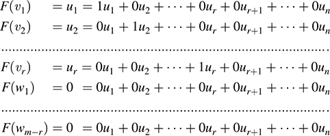
Thus, the matrix of F in the above bases has the required form.

SUPPLEMENTARY PROBLEMS

Matrices and Linear Operators

6.37.   Let F: R² → R² be defined by F(x, y) = (4x + 5y, 2x y).

(a) Find the matrix A representing F in the usual basis E.

(b) Find the matrix B representing F in the basis S = {u₁, u₂} = {(1, 4), (2, 9)}.

(c) Find P such that B = P^–1 AP.

(d) For υ = (a, b), find [υ]_S and [F (υ)]_S. Verify that [F]_S[υ]_S = [F(υ)_S.

6.38.   Let A: R² → R² be defined by the matrix

(a) Find the matrix B representing A relative to the basis S = {u₁, u₂} = f(1, 3), (2, 8)}. (Recall that A represents the mapping A relative to the usual basis E.)

(b) For υ = (a, b), find [υ]_S and [A(υ)_S.

6.39.   For each linear transformation L on R², find the matrix A representing L (relative to the usual basis of R²):

(a) L is the rotation in R² counterclockwise by 45°.

(b) L is the reflection in R² about the line y = x.

(c) L is defined by L (1, 0) = (3, 5) and L (0, 1) = (7, – 2).

(d) L is defined by L (1, 1) = (3, 7) and L (1, 2) = (5, –4).

6.40.   Find the matrix representing each linear transformation T on R³ relative to the usual basis of R³:

(a) T (x, y, z) = (x, y, 0).

(b) T (x, y, z) = (z, y + z, x + y + z).

(c) T (x, y, z) = (2x – 7y 4z, 3x + y + 4z, 6x – 8y + z).

6.41.   Repeat Problem 6.40 using the basis S = {u₁, u₂, u₃} = {(1, 1, 0), (1, 2, 3), (1, 3, 5)}.

6.42.   Let L be the linear transformation on R³ defined by

(a) Find the matrix A representing L relative to the usual basis of R³.

(b) Find the matrix B representing L relative to the basis S in Problem 6.41.

6.43.   Let D denote the differential operator; that is, D(f(t)) = df/dt. Each of the following sets is a basis of a vector space V of functions. Find the matrix representing D in each basis:

6.44.   Let D denote the differential operator on the vector space V of functions with basis S = {sin θ, cos θ}.

(a) Find the matrix A = [D]_S.

(b) Use A to show that D is a zero of f(t) = t² + 1.

6.45.   Let V be the vector space of 2 ′ 2 matrices. Consider the following matrix M and usual basis E of V:

Find the matrix representing each of the following linear operators T on V relative to E:

(a) T (A) = MA.

(b) T (A) = AM.

(c) T (A) = MA – AM.

6.46.   Let 1_V and 0_V denote the identity and zero operators, respectively, on a vector space V. Show that, for any basis S of V, (a) [1_V]_S = I, the identity matrix. (b) [0_V]_S = 0, the zero matrix.

Change of Basis

6.47.   Find the change-of-basis matrix P from the usual basis E of R² to a basis S, the change-of-basis matrix Q from S back to E, and the coordinates of υ = (a, b) relative to S, for the following bases S:

(a) S = {(1, 2), (3, 5)}.

(b) S = {(1, – 3), (3, – 8)}.

(c) S = {(2, 5), (3, 7)}.

(d) S = {(2, 3), (4, 5)}.

6.48.   Consider the bases S = {(1, 2), (2, 3)g and S′ = {(1, 3), (1, 4)g of R². Find the change-of-basis matrix:

(a) P from S to S′.

(b) Q from S′ back to S.

6.49.   Suppose that the x-axis and y-axis in the plane R² are rotated counterclockwise 30° to yield new x′-axis and y ⁰-axis for the plane. Find

(a) The unit vectors in the direction of the new x′-axis and y′-axis.

(b) The change-of-basis matrix P for the new coordinate system.

(c) The new coordinates of the points A (1, 3), B (2, 5), C (a, b).

6.50.   Find the change-of-basis matrix P from the usual basis E of R³ to a basis S, the change-of-basis matrix Q from S back to E, and the coordinates of υ = (a, b, c) relative to S, where S consists of the vectors:

(a) u₁ = (1, 1, 0), u₂ = (0, 1, 2), u₃ = (0, 1, 1).

(b) u₁ = (1, 0, 1), u₂ = (1, 1, 2), u₃ = (1, 2, 4).

(c) u₁ = (1, 2, 1), u₂ = (1, 3, 4), u₃ = (2, 5, 6).

6.51.   Suppose S₁, S₂, S₃ are bases of V. Let P and Q be the change-of-basis matrices, respectively, from S₁ to S₂ and from S₂ to S₃. Prove that PQ is the change-of-basis matrix from S₁ to S₃.

Linear Operators and Change of Basis

6.52.   Consider the linear operator F on R² defined by F(x, y) = (5x + y, 3x – 2y) and the following bases of R²:

(a) Find the matrix A representing F relative to the basis S.

(b) Find the matrix B representing F relative to the basis S′.

(c) Find the change-of-basis matrix P from S to S′.

(d) How are A and B related?

6.53.   Let A: R² → R² be defined by the matrix 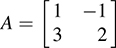. Find the matrix B that represents the linear operator

A relative to each of the following bases: (a) S = {(1, 3)^T, (2, 5)^T}. (b) S = {(1, 3)^T, (2, 4)^T}.

6.54.   Let F: R² → R² be defined by F(x, y) = (x − 3y, 2x − 4y). Find the matrix A that represents F relative to each of the following bases: (a) S = {(2, 5), (3, 7)}. (b) S = {(2, 3), (4, 5)}.

6.55.   Let A: R³ → R³ be defined by the matrix . Find the matrix B that represents the linear operator A relative to the basis S = {(1, 1, 1)^T, (0, 1, 1)^T, (1, 2, 3)^T}.

Similarity of Matrices

6.56.   Let and .

(a) Find B = P⁻¹AP.

(b) Verify that tr(B) = tr(A).

(c) Verify that det(B) = det(A).

6.57.   Find the trace and determinant of each of the following linear maps on R²:

(a) F(x, y) = (2x − 3y, 5x + 4y).

(b) G(x, y) = (ax + by, cx + dy).

6.58.   Find the trace and determinant of each of the following linear maps on R³:

(a) F(x, y, z) = (x + 3y, 3x − 2z, x − 4y − 3z).

(b) G(x, y, z) = (y + 3z, 2x − 4z, 5x + 7y).

6.59.   Suppose S = {u₁, u₂} is a basis of V, and T: V → V is defined by T(u₁) = 3u₁ − 2u₂ and T(u₂) = u₁ + 4u₂. Suppose S′ = {w₁, w₂} is a basis of V for which w₁ = u₁ + u₂ and w₂ = 2u₁ + 3u₂.

(a) Find the matrices A and B representing T relative to the bases S and S′, respectively.

(b) Find the matrix P such that B = P⁻¹AP.

6.60.   Let A be a 2 × 2 matrix such that only A is similar to itself. Show that A is a scalar matrix, that is, that .

6.61.   Show that all matrices similar to an invertible matrix are invertible. More generally, show that similar matrices have the same rank.

Matrix Representation of General Linear Mappings

6.62.   Find the matrix representation of each of the following linear maps relative to the usual basis for Rⁿ:

(a) F: R³ → R² defined by F(x, y, z) = (2x − 4y + 9z, 5x + 3y − 2z).

(b) F: R² → R⁴ defined by F(x, y) = (3x + 4y, 5x − 2y, x + 7y, 4x).

(c) F: R⁴ → R defined by F(x₁, x₂, x₃, x₄) = 2x₁ + x₂ − 7x₃ − x₄.

6.63.   Let G: R³ → R² be defined by G(x, y, z) = (2x + 3y z, 4x y + 2z).

(a) Find the matrix A representing G relative to the bases

(b) For any υ = (a, b, c) in R³, find [υ]_S and [G(υ)]_S′.

(c) Verify that A[υ]_S = [G(υ)]_S′.

6.64.   Let H: R² → R² be defined by H(x, y) = (2x + 7y, x − 3y) and consider the following bases of R²:

(a) Find the matrix A representing H relative to the bases S and S′.

(b) Find the matrix B representing H relative to the bases S′ and S.

6.65.   Let F: R³ → R² be defined by F(x, y, z) = (2x + y z, 3x − 2y + 4z).

(a) Find the matrix A representing F relative to the bases

(b) Verify that, for any υ = (a, b, c) in R³, A[υ]_S = [F(υ)]_S′.

6.66.   Let S and S′ be bases of V,and let 1_V be the identity mapping on V. Show that the matrix A representing 1_V relative to the bases S and S′ is the inverse of the change-of-basis matrix P from S to S′; that is, A = P⁻¹.

6.67.   Prove (a) Theorem 6.10, (b) Theorem 6.11, (c) Theorem 6.12, (d) Theorem 6.13. [Hint: See the proofs of the analogous Theorems 6.1 (Problem 6.9), 6.2 (Problem 6.10), 6.3 (Problem 6.11), and 6.7 (Problem 6.26).]

Miscellaneous Problems

6.68.   Suppose F: V → V is linear. A subspace W of V is said to be invariant under F if F(W) ⊆ W. Suppose W is invariant under F and dim W = r. Show that F has a block triangular matrix representation where A is an r × r submatrix.

6.69.   Suppose V = U + W, and suppose U and V are each invariant under a linear operator F: V → V. Also, suppose dim U = r and dim W = S. Show that F has a block diagonal matrix representation where A and B are r × r and s × s submatrices.

6.70.   Two linear operators F and G on V are said to be similar if there exists an invertible linear operator T on V such that G = T⁻¹ ∘ F ∘ T. Prove

(a) F and G are similar if and only if, for any basis S of V, [F]_S and [G]_S are similar matrices.

(b) If F is diagonalizable (similar to a diagonal matrix), then any similar matrix G is also diagonalizable.

ANSWERS TO SUPPLEMENTARY PROBLEMS

Notation: M = [R₁; R₂; …] represents a matrix M with rows R₁, R₂, ….

6.37.   (a) A = [4, 5; 2, −1; (b) B = [220, 487; −98, −217]; (c) P = [1, 2; 4, 9]; (d) [υ]_S = [9a − 2b, −4a + b]^T and [F(υ)]_S = [32a + 47b, −14a − 21b]^T

6.38.   

6.39.   

6.40.   (a) [1, 0, 0; 0, 1, 0; 0, 0, 0]; (b) [0, 0, 1; 0, 1, 1; 1, 1, 1];

(c) [2, −7, −4; 3, 1, 4; 6, −8, 1]

6.41.   (a) [1, 3, 5; 0, −5, −10; 0, 3, 6]; (b) [0, 1, 2; 1, 2, 3; 1, 0, 0];

(c) [15, 65, 104; 49, −219, −351; 29, 130, 208]

6.42.   (a) [1, 1, 2; 1, 3, 2; 1, 5, 2]; (b) [0; 2, 14, 22; 0, −5, −8]

6.43.   (a) [1, 0, 0; 0, 2, 1; 0, 0, 2]; (b) [0, 1, 0, 0; 0; 0, 0, 0, −3; 0, 0, 3, 0]; (c) [5, 1, 0; 0, 5, 2; 0, 0, 5]

6.44.   (a) A = [0, −1; 1, 0;] (b) A² + I = 0

6.45.   (a) [a, 0, b, 0; 0, a, 0, b; c, 0, d, 0; 0, c, 0, d];

(b) [a, c, 0, 0; b, d, 0, 0; 0, 0, a, c; 0, 0, b, d];

(c) [0, −c, b, 0; −b, a − d, 0, b; c, 0, d − a, −c; 0, c, −b, 0]

6.47.

6.48.   (a) P = [3, 5; 1, −2 ×]; (b) Q = [2, 5; 1, −3]

6.49.   

6.50.   P is the matrix whose columns are u₁, u₂, u₃, Q = P⁻¹, [υ] = Q[a, b, c^T:

6.52.   (a) [23, −39; 15, 26]; (b) [35, 41; 27, −32]; (c) [3, 5; 1, −2]; (d) B = P⁻¹AP

6.53.   

6.54.   

6.55.   [10, 8, 20; 13, 11, 28; 5, −4, −10]

6.56.   (a) [34, 57; 19, 32]; (b) tr(B) = tr(A) = −2; (c) det(B) = det(A) = −5

6.57.   (a) tr(F) = 6, det(F) = 23; (b) tr(G) = a + d, det(G) = ad − bc

6.58.   (a) tr(F) = −2, det(F) = 13; (b) tr(G) = 0, det(G) = 22

6.59.   (a) A = [3, 1; −2, 4], B = [8, 11; 2, −1]; (b) P = [1, 2; 1, 3]

6.62.   (a) [2, −4, 9; 5, 3, −2 ×]; (b) [3, 5, 1, 4; 4, −2, 7, 0]; (c) [2, 1, −7, −1]

6.63.   (a) [9, 1, 4; 7, 2, 1]; (b) [υ]_S = [−a + 2b − c, 5a − 5b + 2c, −3a + 3b − c]^T, and [G(υ)]_S′ = [2a − 11b + 7c, 7b − 4c]^T

6.64.   (a) A = [47, 85; −38, −69]; (b) B = [71, 88; 41, −51]

6.65.   A = [3, 11, 5; −1, −8, −3]