1. Variation in life history among species and the notion of trade-offs
2. Key life history patterns and associated trade-offs
The term life history summarizes the timing and magnitude of growth, reproduction, and mortality over the lifetime of an individual organism. Important features of an individual’s life history include the age or size at which reproduction begins, the relationship between size and age, the number of reproductive events over the individual’s lifetime, the size and number of offspring produced at each reproductive event, the sex ratio of offspring, the chance that the individual dies as a function of age or size, and the individual’s lifespan or longevity (the time elapsed between the birth and death of the individual). Although all of these features (so-called life history traits) describe individuals, some are more easily understood when viewed as aggregate properties of a population of individuals. This is particularly true of mortality and lifespan. Each individual dies once, at a certain age. But in a population of identical individuals, some may die at a young age and some at an old age. By imagining that the fraction of this population that is still alive at a given age also represents the probability that an average individual survives to that age, we see that the chance of survival to a given age, which is the converse of the chance of dying, or mortality, is a property of an individual. Similarly, we can envision the average lifespan (or “life expectancy”) even though each individual has a single age at death. All sunflowers and the vast majority of sequoia seedlings die before reaching one year of age. Yet in a sequoia population, individuals have the potential to live for several millennia, which distinguishes sequoias from sunflowers.
fertility. The number of daughters to which a female gives birth during a specified age interval
geometric mean. The nth root of the product of n numbers
iteroparity. A reproductive pattern in which individuals reproduce more than once in their lives
life table. A table summarizing age-specific survivorship and fertility used to calculate the net reproductive rate
net reproductive rate. The average number of daughters to which a newborn female gives birth over her entire life
semelparity. A reproductive pattern in which individuals reproduce only once in their lives
survivorship. The probability that a newborn survives to or beyond a specified age
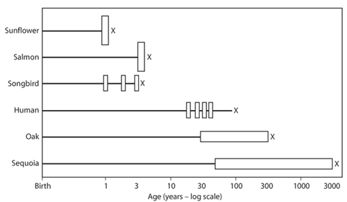
As for the difference in life expectancy between sunflowers and sequoias, each of the key life history traits varies 1000-fold or more among species, as illustrated in figure 1. Life history traits also vary among individuals of the same species. The fundamental question in ecological and evolutionary studies of life history is: why is there so much variation in life history traits among and within species?
To answer this question, we start by recognizing that life history features are traits just like any other (e.g., coloration, bill shape, cold tolerance, body size, etc.) that can be acted on by natural selection. Moreover, variation in life history traits among individuals in a population often has a genetic basis, so genotypes favored by natural selection can potentially increase in frequency from one generation to the next. If life history traits are genetically based and subject to selection, evolution of life history might be expected to lead to an organism that begins reproducing immediately after birth and produces a large number of well-provisioned offspring in a series of reproductive events throughout an infinitely long life (such an organism has been termed a “Darwinian monster” because it would quickly displace all other species from Earth). The reason we do not see Darwinian monsters even though life history traits evolve is that different life history traits are not independent.
Figure 1. Diversity of life histories for six representative species, three plants (sunflower, oak, and sequoia trees) and three animals (salmon, songbird, and human). Rectangles show reproductive events; height of each rectangle indicates the magnitude of reproductive effort (separate reproductive events are merged for oaks and sequoias). An “x” marks the age at death of an adult. Note that age is on a logarithmic scale; sequoias can live 3000 times longer than sunflowers.
Because the resources that an organism has available to invest in maintenance and survival, in growth, and in reproduction are always limited, life history evolution is constrained by trade-offs: a greater investment in one life history trait must come at the expense of a smaller investment in one or more other life history traits. Trade-offs between many different pairs of life history traits have been documented, and we will see several examples in the following section of this article. In recognizing trade-offs, we no longer expect that evolution will produce Darwinian monsters, but rather that natural selection will balance, for example, improvements in reproduction with reductions in survival. On one hand, the optimal balance may depend on features of the environment the organism occupies. On the other hand, multiple combinations of life history traits may produce equally fit organisms. Both provide explanations for the diversity of life histories we see among Earth’s biota.
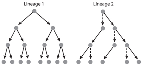
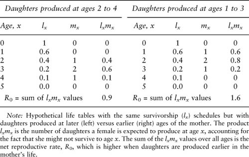
All else being equal, an organism should begin reproducing as soon as possible, for two reasons. First, because of factors such as predators and diseases, adverse weather, or genetic defects, the organism may not survive for long, so delaying reproduction carries the risk of dying before reproducing. This advantage of early reproduction is easily illustrated with a basic demographic tool, the life table (table 1). A life table has two principal columns, survivorship, usually denoted lx, which is the probability that a newborn female survives to age x or older, and fertility, usually denoted mx, which is the average number of daughters a mother of age x produces over the next age interval (note that life tables typically track females only). One use of a life table is to compute the average number of daughters a female will produce over her entire life, which is called the net reproductive rate and is usually denoted R0. Natural selection can be expected to favor production of more daughters. As shown in table 1, for a fixed set of lx values, fertility skewed toward earlier ages will lead to a higher R0 simply because females will be more likely to survive to reproduce. The second reason why early reproduction is advantageous is that daughters produced earlier will themselves begin reproducing sooner than will daughters produced later in the mother’s life. If we think of a mother and her female descendents as a lineage, a lineage founded by an early-reproducing mother will grow faster than will the lineage of a later-reproducing founder, even if both lineages have the same R0 (figure 2).
However, the production of offspring costs resources that the parent could use for other purposes, such as growth. Individuals that reproduce early in life may grow less rapidly, a trade-off between early reproduction and early growth that may prevent early reproducers from reaching a large final size. Moreover, because larger individuals often have both a greater chance of surviving and a greater reproductive potential, early reproduction may also be involved in tradeoffs with later survival and later reproduction. If reproductive capacity increases rapidly as the size of an organism increases, delaying reproduction in order to achieve a larger size may allow an individual to produce more offspring over its entire life despite the advantages of early reproduction illustrated in table 1 and figure 2.
Figure 2. Growth of two female lineages. In Lineage 1, each mother produces two daughters in her first year and then dies. In Lineage 2, each mother produces one daughter in her first and one in her second year and then dies. For both lineages, R0=2, but the first lineage grows faster. Circles are females, dashed vertical arrows show survival of the same female, and solid arrows show production of daughters.
Delaying reproduction in order to grow more rapidly is especially important for males of species with territorial breeding systems. For example, the victors of fights between male elephant seals gain nearly exclusive reproductive access to harems of females. Because small males have little chance of winning fights, young males invest energy in growing larger rather than in futile attempts to breed. In contrast, females do not need to win fights to breed, so they begin reproducing several years earlier in life than do males. Thus, males and females of the same species may face different trade-offs between early reproduction and growth.
Interestingly, a breeding system in which males delay reproduction to grow large enough to win male–male contests may open the door for alternative mating strategies used by smaller or younger males. In many fish species, small males known as satellites may mimic females or use other methods to sneak into the territory of a mating pair in order to fertilize some of the female’s eggs when she releases them into the water. Satellites also occur in other animal groups (including lizards). Satellites can increase in a population when they are rare, because there are many territorial males to “parasitize,” but their success declines as they become a larger proportion of the population. They may achieve reproductive success similar to that of territorial males, or they may be making the best of a small size caused by genetic or environmental factors.
Constant Environments
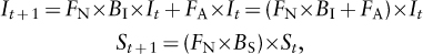
Once an individual becomes reproductively mature, it can breed only once (semelparous species), as in sunflowers and salmon, or breed multiple times (iteroparous species). Intuitively, we might think that if breeding once is good, breeding more than once is better. But Lamont C. Cole pointed out in 1954 that the lineage of an immortal organism that reproduces every year would grow at the same rate as the lineage of an organism that reproduces only once at 1 year of age and then dies, but produces just one more offspring than does the iteroparous organism at each of its breeding events (it is easy to modify figure 2 to see how Cole’s claim might be true). More than one additional offspring would give the advantage to the semelparous organism, and if the cost of investing in survival is high, an organism that reproduced once and then died might be able to achieve even higher reproduction (note that we have just assumed a survival–reproduction trade-off). Thus, Cole claimed that iteroparity was more paradoxical than semelparity. Other ecologists showed later that Cole’s result requires that adults and newborn offspring have the same chance of surviving each year, which we now demonstrate with a simple mathematical model. If It and St are the numbers of individuals in the iteroparous and semelparous lineages in year t, then It+1 and St+1, the numbers in the two lineages the following year, are predicted by
Table 1. Hypothetical life tables
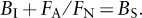
where FN and FA are the fractions of newborns and adults surviving the year, and BI and BS are the numbers of newborns produced by each iteroparous and semelparous organism each year. There is no FA term in the equation for the semelparous lineage because individuals die after breeding. The two lineages will grow at the same rate if the terms in parentheses in the two equations are equal, that is, if

or, dividing both sides of the equation by FN, if
If instead the left side of the preceding equation is larger than the right side, the iteroparous lineage will grow faster. Note that if the same fraction of adults and newborns survive the year (i.e., if FA = FN), we obtain Cole’s result (because the semelparous organisms are producing one more newborn than are the iteroparous organisms). However, because newborns are smaller and often more vulnerable than adults, for many species and environments, a smaller fraction of newborns than adults will survive. Because FA/FN may then be substantially greater than 1, semelparous reproduction may need to be a good deal greater to achieve a fitness equal to that of the iteroparous lineage. Thus, an important advantage of iteroparity is that it capitalizes on the greater value of adults, as measured by their higher survival rates, even at the expense of lower offspring production at each breeding event.
Variable Environments
In the preceding section, we assumed that newborn survival is the same every year. Long-lived adults are even more valuable in an environment in which newborn survival varies from year to year, as is likely to occur for many species and environments. Imagine that there are two kinds of years, good and bad, for newborn survival. Assume that in good years, FN = 0.5 + D, and in bad years, FN = 0.5 − D; by increasing the number D, we increase the contrast between good and bad years. If D = 0, 50% of newborns survive every year. If D = 0.5, all newborns survive in good years, and none survive in bad years (higher values of D are meaningless because the survival fraction cannot be less than 0 or greater than 1). If we assume that good and bad years are equally frequent but occur at random, then regardless of the value of D, the average newborn survival across years is 0.5.
If newborn survival varies from year to year, the terms in parentheses in the equations we used above to predict the growth of iteroparous and semelparous lineages, which represent the annual lineage growth rates, also vary from year to year.
Note that to get It+2, the size of the iteroparous lineage in year t+2, we would first compute If+1 by multiplying It by the annual growth rate for the iteroparous lineage in year t [which would be (0.5 + D)×BI+FA if year t were a good year and (0.5 – D)×BI+FA if year t were a bad year] and then multiply the result by the annual growth rate for year t+1 (which again might be a good or a bad year). Thus, over a period of years, the size of a lineage (either iteroparous or semelparous) is determined by the product of the annual lineage growth rates. If good and bad years are equally likely, then over a long period of years, close to half of the years will be good and half will be bad, and in a typical 2-year period one will be good and one will be bad. Thus, the growth of the iteroparous lineage over a typical 2-year period will be determined by the product of the good-year and bad-year growth rates, [(0.5 + D) × BI+FA] × [(0.5 – D) × BI+FA], and the growth over a typical 1-year period will be the square root of this product. Similarly, the typical 1-year growth rate of the semelparous lineage will be the square root of the product [(0.5 + D) × BS] × [(0.5 — D) × BS]. These typical growth rates represent the geometric means of the annual growth rates. (The geometric mean of two numbers is the square root of their product, whereas the more familiar average or arithmetic mean is one-half of their sum.) Because lineage growth is a multiplicative process, the geometric mean is a more appropriate measure of typical annual growth.
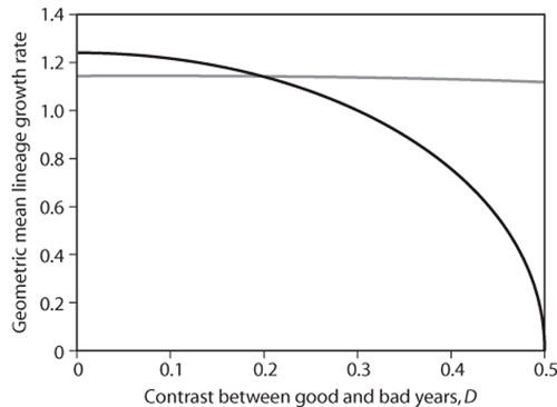
Now let us set FA to 0.9 (90% of adults survive a year) and BI and BS to 0.5 and 2.5, respectively (the semelparous organism produces on average two more offspring per year than does the iteroparous organism). If D = 0, all years are the same, and the annual growth rate of the iteroparous lineage, BI × FN+FA = 0.5 × 0.5 + 0.9 = 1.15, is less than the annual growth rate of the semelparous lineage BS × FN = 2.5 × 0.5 = 1.25. Thus, in a constant environment characterized by the survival and reproductive rates we have chosen, the semelparous lineage outperforms the iteroparous lineage. But what happens as we increase the contrast between good and bad years by increasing the value of D? As figure 3 illustrates, the semelparous lineage continues to grow faster than the iteroparous lineage when year-to-year variability in newborn survival (as determined by D) is low. However, the growth rates of both lineages decline as D increases, but much more so for the semelparous lineage, so that once D exceeds 0.2, the iteroparous lineage outgrows the semelparous lineage. Note that we have not changed the average newborn survival rate, so the switch in relative performance of the two lineages shown in figure 3 is driven entirely by the increase in variability of newborn survival. The presence of long-lived adults in the iteroparous lineage allows it to persist during years when few or no newborns survive. In contrast, persistence of the semelparous lineage requires that at least some newborns survive every year. That is why the geometric mean growth rate of the semelparous lineage is zero when D = 0.5 and its bad-year annual growth is zero; a single zero will cause the product of annual growth rates to be zero because a single year in which all newborns die will cause extinction of the lineage.
Thus, iteroparity, even at a cost of reduced annual reproduction, can be favored when newborn survival is low on average and/or is highly variable from year to year. Essentially, long-lived adults spread their reproductive efforts over multiple years, so their lifetime reproductive success is less sensitive to a single bad year. Although iteroparity is one life history adaptation to randomly varying environments, semelparous species also possess life history adaptations to environmental variability, namely dormancy and diapause, which we omitted from our simple model. Annual plants, by definition, reproduce only once, but many of them produce seeds of which a fraction lie dormant in the soil for one or more years. Because the offspring of a parent plant then germinate in different years, the parent is effectively spreading its reproduction over several years, just as an iteroparous organism does, thus reducing its sensitivity to a single bad year in which all seedlings die and increasing its geometric mean fitness. Similarly, many insects and other invertebrates can remain in an inactive diapause state as adults for more than a year, allowing the set of offspring of a single mother to sample different years even though each offspring reproduces only once.
Figure 3. The typical annual growth rates of the semelparous lineage (shown as a black line) and of the iteroparous lineage (shown as a gray line) when newborn survival varies randomly from year to year. The typical growth rate is measured as the geometric mean, and the contrast in newborn survival between good and bad years increases as D increases.
We assumed above that only newborn survival varied from year to year, but in reality, the survival, growth, and reproduction of individuals of all ages are likely to vary. In a completely unpredictable environment, year-to-year variability in all of these life history traits will depress the geometric mean growth rate of a lineage, just as variability in newborn survival does in figure 3, but variability in traits such as adult survival that make large contributions to the lineage growth rate will be more detrimental than variability in less influential traits. Across many species, there is growing evidence that the most influential life history traits vary less from year to year than do less influential traits, suggesting that mechanisms have evolved that buffer the life histories of those organisms against the most detrimental types of variability.
However, not all year-to-year variability in life history traits is detrimental. Many environments are only partly unpredictable. For example, in fire-prone ecosystems, it may be difficult to predict whether a fire will occur in a given year, but once a fire has occurred, conditions of abundant resources, low competition, and low likelihood of additional disturbance may be quite predictable until enough fuel has accumulated to allow the next fire to occur. Many species inhabiting such disturbance-dominated systems have evolved timing of the phases in their life histories to exploit this environmental predictability. For example, many fire-adapted plants produce seeds that germinate only in the period soon after a fire, so their offspring can take advantage of abundant postfire resources. Conversely, reproduction of these plants is often restricted to late in the interfire interval, after plants have grown to reproductive size and when their seeds will be poised to exploit the next interfire interval. In these species, among-year variation in life history traits reflects adaptation to multiyear environmental cycles rather than the detrimental influence of environmental variability.
Even iteroparous organisms eventually die. Moreover, for many species, the chance of dying in a given interval of time may initially decline after birth as newborns grow to a less vulnerable size or as those with developmental defects die, but it eventually increases as individuals reach more advanced ages. The process of aging is defined as an increase in mortality risk late in life. As we would expect that the ability to continue living and reproducing would be favored by natural selection, why does aging occur? Peter B. Medawar argued, and William D. Hamilton showed mathematically, that the ability of natural selection to weed out genes that increase mortality or decrease fertility declines with an organism’s age. The reason for this decline in the strength of selection is that even individuals with good genes are increasingly likely to have died from external causes, such as predators or bad weather, as age increases. Therefore, few individuals will still be alive to enjoy the advantage of decreased mortality risk or increased fertility at advanced ages, whereas most individuals will benefit from increases in early-life survival or fertility. Two types of genes may underlie an increase in mortality or decrease in fertility with age. Detrimental genes that are expressed only late in life would experience only weak selection against them and so would tend to accumulate in the genome. Genes that have beneficial effects on survival or fertility early in life but detrimental effects late in life would be maintained because positive selection for their early effects would overwhelm negative selection for their late effects. The former type of genes play a role in Peter Medawar’s mutation accumulation theory of aging, whereas the latter type of genes are central to George C. Williams’ antagonistic pleiotropy theory of aging. There is evidence that both types of genes may be present in the same organisms.
For many organisms, including fruit flies, some plants, and humans, the risk of mortality reaches a plateau rather than continuing to increase at very advanced ages. A mortality plateau could arise because individuals that are frail from genetic or environmental factors are increasingly likely to have already died as age increases. But as Hamilton’s theory shows that natural selection will be powerless to eliminate detrimental genes expressed at all ages past the age at which reproduction ceases, detrimental late-acting genes could simply be maintained at intermediate frequencies by a balance between the nonselective evolutionary forces of mutation and genetic drift.
Although Hamilton’s work predicts that there will be no selection to reduce mortality once reproduction ceases, that work only accounts for offspring directly produced by a mother. However, mothers can also contribute to the growth of their lineage by providing direct care to their granddaughters or by providing information that improves the quality of care their daughters provide to their own offspring. These direct and indirect transfers across two generations may explain why, in social species such as primates, mortality does not increase rapidly once a female ceases to give birth.
Whether an organism reproduces once or more than once, the resources it invests in a single breeding event can be used to produce a single large offspring, or those resources can be divided to produce more than one, but smaller, offspring. The trade-off between the size and number of offspring is a fundamental constraint on life history. Producing more offspring will cause a lineage to grow faster, but not if each offspring is too small to have a good chance of surviving. Therefore, the best solution in the face of a size–number trade-off is to produce the number (and therefore size) of offspring at which the product of the offspring number and the size-dependent probability that each offspring survives is at a maximum. Other factors may skew the optimum solution toward more and smaller offspring. For example, trees with seeds dispersed by wind typically make many small seeds. Even though the small seedling emerging from each seed has a low chance of surviving, by increasing the area reached by its windblown seeds, a mother plant will be more likely to place at least some of its seeds in sites suitable for seedling growth and survival, even if those sites are few and far between.
A large number of studies have addressed the question of why most female birds lay fewer eggs in each nest than the maximum number observed for the species. Why do lineages that produce more eggs per nest not come to replace lineages that produce fewer eggs per nest? David L. Lack proposed that birds should maximize the number of offspring surviving to leave the nest rather than the number of eggs per nest. Because the parents can provide less food to each chick when a nest contains many chicks, the chance that each chick survives declines with the number of eggs (and therefore chicks) in a nest. As a result, the product of the number of eggs per nest and the probability that the chick hatching from each egg survives to leave the nest is usually highest at an intermediate egg number. However, this number is often higher than the average number of eggs actually observed in nest. Birds may lay fewer eggs than Lack’s argument predicts because excessive investment in one nest reduces the parents’ chance of survival or their future reproductive success. That is, trade-offs between current reproduction and future survival or future reproduction may constrain the amount invested in a single bout of reproduction.
See also chapters I.13, I.14, and II.1 in this volume.
Roff, D. A. 1992. The Evolution of Life Histories. New York: Chapman & Hall.
Stearns, S. C. 1992. The Evolution of Life Histories. Oxford: Oxford University Press. Two excellent and comprehensive overviews of the field.
Cole, L. C. 1954. The population consequences of life history phenomena. Quarterly Review of Biology 103: 103–137. A classic paper that spurred research into reproductive patterns and longevity.
Hamilton, W. D. 1966. Moulding of senescence by natural selection. Journal of Theoretical Biology 12: 12–45. Although rather mathematical, this paper is the basis for most evolutionary theories of aging.
Partridge, L., and D. Gems. 2006. Beyond the evolutionary theory of ageing, from functional genomics to evo-gero. Trends in Ecology and Evolution 21: 334–340. A recent review of genetic causes of aging.
Rose, M. R. 1991. Evolutionary Biology of Aging. New York: Oxford University Press.
Rose, M. R., C. L. Rauser, L. D. Mueller, and G. Benford. 2006. A revolution for aging research. Biogerontology 7: 269–277. A review of the evidence for and causes of mortality plateaus.
Godfray, H.C.J., L. Partridge, and P. H. Harvey. 1991. Clutch size. Annual Review of Ecology and Systematics 22: 409–429. Emphasizes determinants of offspring number in organisms other than birds.
Lack, D. L. 1954. Natural Regulation of Animal Numbers. Oxford: Oxford University Press. This book includes Lack’s argument for why birds should lay fewer than the maximum number of eggs per nest.