Chapter 14. Rendering and Compositing
In this chapter, we move into the final stages of the projects as we turn each of the scenes into rendered images and tweak them to look their best. We begin by looking at Blender’s render settings, both for Blender Internal and Cycles, to determine how to get the best render in the shortest time possible. Following that discussion, I’ll cover using Blender’s node-based compositor to further refine, adjust, and grade these renders into final images. Finally, we’ll make a few tweaks to the renders in GIMP.
The Render Tab
We touched on the Render tab of the Properties editor when we used it to bake textures in Chapter 10. In this chapter, we’ll examine the other settings available in this tab. Many of these depend on which renderer is being used—Blender Internal or Cycles—so we will look at each in turn.
Rendering with Blender Internal
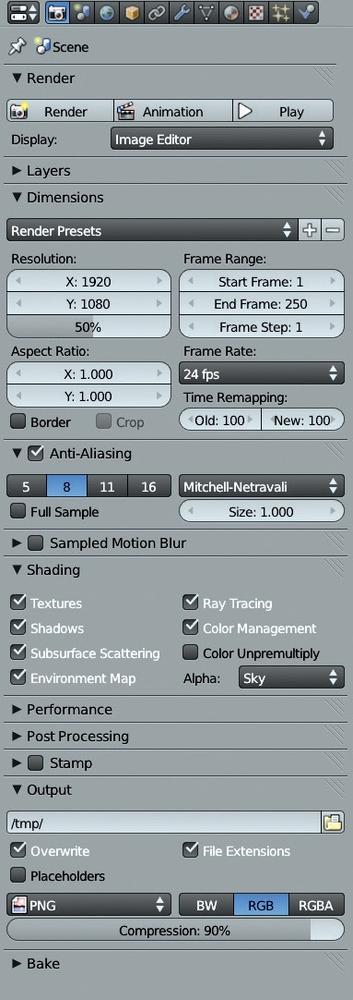
The Render tab in Blender Internal is shown in Figure 14-1. Let’s look at the settings available in each panel.
Render Panel
This contains buttons for rendering your animation and playing back the results.
Image/Animation. These buttons render the current frame (F12) or every frame in the range set by the Frame Range settings in the Dimensions panel as an animation (CTRL-F12). You can play back the rendered animation with the play button.
Display. Display lets you set where the rendered image will appear. The Image editor option will render the image in an available UV Image editor if possible, or it will temporarily switch one of the other editors into a UV Image editor during rendering if necessary. The other options allow you to render full screen, in a new window, or in the background (Keep UI).
Layers Panel
The Layers panel contains tools and options for creating different render layers and for choosing which scene layers contribute to your final renders. At the top of the panel, the Layer selector lets you select the render layer to work on. Use the checkboxes on the right to enable or disable rendering particular layers; use the + and – buttons on the right to add or delete render layers.
Name. This allows you to name the selected layer.
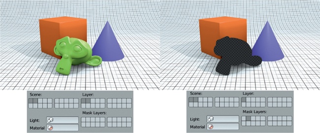
Scene/Layer/Mask Layer. These three sets of checkboxes let you choose which scene layers are used in your final renders and how. Enabling a layer under Scene turns the layer on in the 3D Viewport (just as the layers checkboxes in the 3D viewport header do). Layers must be checked under Scene to be renderable. Enable layers under Layer to make them render for the currently selected render layer; you can have multiple layers turned on under Scene, but only those checked under Layer will be rendered. Layers checked under Mask (but not under Layer) will mask out geometry on other layers, as shown in Figure 14-2.
Light. The Light option lets you specify a group of lights to be treated as the only lights in the scene when rendered.
Material. As discussed in Clay Renders and Material Override, the Materials option lets you override the materials for a scene with a single material when rendering. We used this option in Chapter 13 to produce a clay render of the Bat Creature project in order to test the lighting.
Include. This offers a number of checkboxes that detail the types of surfaces and effects to be rendered with this layer. For example, you can turn on or off the rendering of z-transparent materials, fur, or solid materials.
Passes. Within a layer, Blender can render other kinds of information and split up aspects of an image into different passes, such as shadows, environment lighting, and z-depth (the distance from the camera). This pass then contains only that data that can be used in compositing the final image. For example, you could use the z-depth pass as the input for a Defocus node to create depth of field, or you could use an ambient occlusion pass to add extra shadows to an image. Use the checkboxes under Passes to enable or disable various passes. Some passes can be excluded from the main render pass by toggling the camera icon to the right of the pass’s name.
Dimensions
This panel lets you set the dimensions in time (frames) and space (resolution) of your render or animation. The Resolution settings let you choose the size of your final render, while the Frame Range settings are used to specify the number of frames in your animation. Aspect Ratio sets the aspect ratio for the pixels in the image (some video formats use nonsquare pixels, but for stills, always use square 1:1 ratio pixels).
You can use the Border and Crop settings to render a small patch of your image rather than the whole thing. To do so, switch to the camera view in the 3D Viewport (NUMPAD 0). Then press SHIFT-B and drag out a rectangle over the area you wish to restrict the render to. This will automatically enable the Border setting. Use the Crop setting to reduce an image’s dimensions to the size of your border region; otherwise, the remaining area will be filled with black.
Anti-Aliasing and Motion Blur
Aliasing is an artifact in a pixel-based image where sharp boundaries may look jagged due to the finite resolution of the image (see Figure 14-3). Aliasing is often most obvious on the outlines of objects or shadows, but it can also crop up in textures or specular highlights. Anti-aliasing addresses this problem by taking multiple subsamples of each pixel with slightly different offsets and blending them, resulting in a smoother-looking boundary, as you can see in the figure.
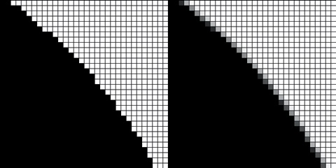
Use the numbers on the left of the Anti-Aliasing panel to determine how many samples will be taken (more samples will result in smoother renders but longer render times). The drop-down menu on the right sets the type of filter used to blend the samples: The default of Mitchell-Netravali gives good results without taking too much sharpness out of the render, but when working with higher-resolution images, try Gaussian. Use the Full Sample option to make Blender maintain each sample separately, even during compositing, which can help with aliasing issues at the compositing stage.
Sampled motion blur is similar to anti-aliasing in that multiple samples are taken per pixel but at different times rather than different locations. This results in motion blur for fast-moving objects once the samples are blended together. (Essentially, the image is rendered multiple times, and the results are blended.) The number of samples is determined by the Motion Samples setting, and the amount of time in frames over which the samples are taken is determined by the Shutter setting.
Shading
The Shading panel lets you turn on and off different rendering options, including Textures, Shadows, Subsurface Scattering, Environment Mapping, and Ray-Tracing options. To speed up renders, turn off unneeded shading options.
The Alpha drop-down menu lets you choose how to render the background of your image. Sky renders the sky colors and textures set in your global settings. The Straight Alpha and Premultiplied options render the background of your image as transparent. In the case of Premultiplied, the RGB values of transparent or partially transparent pixels are multiplied by the alpha value on output. This method of encoding alpha values is also referred to as associated alpha and is required for some image formats, like TIFF and PNG. It’s also useful for compositing because combining images this way gives better results, though Blender’s compositor has tools for working with both premultiplied and unpremultiplied alpha. Straight Alpha skips this step and renders unassociated alpha images instead.
Note
If the above discussion on different methods of encoding alpha values seems complex, it’s because it is. I’ve covered it only very briefly here, but it’s actually a pretty deep topic. For more information, try searching http://www.blender.org/ and the Blender wiki for Color Management.
Performance
The Performance panel contains a number of options that can affect how fast Blender will render and how much impact rendering will have on your computer’s resources. Blender splits up images to be rendered into multiple tiles, which are then rendered individually. The most important settings are Threads and Tiles. When set to Fixed, these settings let you specify how many tiles will be rendered at once (up to twice the number of processor cores you have).
The Tiles settings determine how the image to be rendered is broken up into tiles along the x- and y-axes. Tiles are rendered one at a time per thread, meaning that if you have eight threads, you will be able to render eight tiles simultaneously.
Tweaking the Tiles settings can make a big difference in your render times. Using too few tiles can mean that processor threads are left idle once all available tiles are being rendered, even if there is plenty of your image left to be rendered. Using too many tiles uses more memory without speeding up the render. The optimum number of tiles is generally between 16 (4×4) and 64 (8×8), with more complex scenes benefiting from more tiles.
The other settings in this panel are even more technical and can usually be left at their defaults. For more on these settings, try http://wiki.blender.org/.
Post-Processing
The Post-Processing settings determine the postprocessing effects applied to your image. The relevant ones are the checkboxes that turn on Compositing and the Sequencer (Compositing should be turned on). Dither adds subtle variation to the colors of pixels, preventing color banding in images with smooth gradients. The Edge setting draws cartoon lines around an image’s geometry, with the strength of the line effect determined by the Threshold setting and the color of the lines determined by the color selector directly below the Threshold setting.
Stamp
The Stamp settings let you stamp your image with data about the render, such as the time it was rendered, the filename, the frame number, and so on. Stamp is often useful when rendering animations, but it’s not of much use to us for our projects.
Output
The Output settings determine where the output of your renders is saved and in what format. Animation frames are saved automatically, but single-frame images must be saved manually. The default output directory (/tmp/ on Mac and Linux systems or the Temp folder on Windows) determines where animation frames are saved, but you can change this to a directory of your choosing. The output format is determined by the drop-down menu, which includes options for what color information to save (black and white, RGB, or RGB and alpha).
Bake
These settings are discussed in detail in Chapter 11.
Rendering with Cycles
Many of the Render tab options remain the same in Cycles, so I will just cover the important differences here.
Sampling
The Sampling panel determines how many samples to calculate for each pixel in the image, which is the main way Cycles determines the quality and noisiness of your final image. The Render and Preview options determine how many samples to render for each pixel in an image before terminating the render. (Use Render for proper renders and Preview for the Cycles preview in the 3D Viewport.) More passes will result in less noise, but the number of passes required to get a noise-free image will vary widely according to the contents of your scene. Seed sets a random value for Cycles to use for sampling, and different seeds will produce different noise patterns.
You can use the Clamp option to prevent fireflies, which are overly bright pixels caused by noise from bright lights or specular highlights. To do so, set the maximum brightness (the clamp value) for a sample to a nonzero number (a value of around 3 works well). This keeps overly bright samples from throwing off the average value of a pixel too much, though it comes at the cost of some accuracy in rendering. (If you leave this at the default of 0, this feature will not be used.)
Light Paths
The Light Paths panel supplements the options in the Samples panel, allowing you to go deeper into how Cycles renders your scene. Specifically the Light Paths panel lets you determine what types of rays to render and how many bounces to calculate before terminating a ray. More bounces give more accurate (and slightly brighter) renders, at the cost of extra render time.
The Transparency, Light Paths, and Bounce settings define the maximum number of light bounces that Cycles will calculate for each type of interaction with light. The Max setting sets the overall maximum number of bounces, while the other settings restrict specific types of rays to fewer bounces. The Min setting for Transparency and Overall Bounces enables early termination of refracted rays, resulting in faster rendering with the loss of some accuracy.
The No Caustics and Shadows options let you turn on and off caustics and ray-traced shadows to speed up rendering. Caustics are rays that have been reflected or refracted by glossy surfaces that then contribute to diffuse illumination. Examples include the bright patterns of sunlight in a swimming pool and light focused by a magnifying glass onto a surface.
Film
You can use the Film panel’s Exposure setting to change the exposure of your render to either brighten or darken scenes overall. (However, it’s best to change the settings on your lamps instead for finer control.) The Transparency checkbox determines whether your background renders as transparent or uses your global settings. The drop-down menu on the right sets the pixel filter type (with the width of the filter below it). Smaller widths produce sharper-looking edges but can cause aliasing. Larger widths give smoother renders at the expense of a small amount of blurring.
Layers
Cycles works much the same as Blender Internal when it comes to layers, but it supplies a different range of passes. Cycles will split up each kind of light ray (diffuse, glossy, and transmission) into separate passes and can split up those passes further into direct and indirect passes. These features can be useful when compositing.
Balancing Render Time and Quality
When rendering any CG scene, the aim is to get the nicest render possible in the shortest amount of time. This can be tricky given the number of variables you can change, all of which affect how long an image will take to render. Still, there are some general principles.
Start simple and be organized. Organize your objects onto layers to make it easier to render different aspects of the scene. Also, make sure you don’t have any unneeded objects in your scene on visible layers when rendering.
Experiment. If your renders are slow, try changing one setting at a time to see what most affects your render times. For example, change a render setting or the number of samples on a lamp. Or enable or disable some aspect of a material, such as subsurface scattering or ray-traced reflections. Changing one thing at a time will let you see exactly what makes the most difference, whereas changing multiple settings forces you to guess which one altered your render time. If you find that something in particular is slowing down your renders without contributing much to the final image, get rid of it.
Minimize surplus geometry. Once you have the camera angle that you want, start getting rid of objects that won’t be seen in your render by deleting them or temporarily shifting them to other layers. This will reduce the amount of geometry Blender has to keep track of when rendering and will speed up your renders! This trick is often helpful when working with environments.
Simplify lighting. Try to simplify the settings on your lamps and see whether you can eliminate some. In particular, look at the shadow settings: Will a smaller shadow-buffer resolution really make much difference, or does a ray-traced lamp need quite so many samples?
As you become more familiar with Blender, you’ll soon learn which settings impact render time for different aspects of scenes. In the meantime, the time you spend experimenting and simplifying your scene will almost always speed up render times.
The Compositor
You’ve pressed F12 to render, and your image is finished, right? Not quite. Now it’s time to post-process the final renders using Blender’s compositor and GIMP. Blender’s compositor is node based and uses the Node editor (which we explored in Editing Node Materials). In this section, I’ll show you how to use the compositor to apply effects such as depth of field, bloom, and color grading and to combine separate render layers into one final image (see Figure 14-5). I’ll also show you how to use GIMP for painting and touch-up.
Rendering and Compositing the Bat Creature
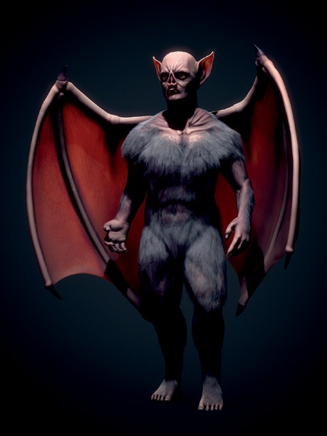
I wanted to show the final Bat Creature on a dark background with a little color grading. To facilitate this, I split the rendering into two layers: one for the fur and one for the rest of the body. I planned to create a simple, dark-colored background in the compositor with a slight vignette to darken the corners and keep the focus on the bat.
Render Layers
As the first step toward splitting the Bat Creature into two render layers, I split my scene into four scene layers. On (scene) layer 1, I placed the body (with Subdivision Surface and Displace modifiers) and the teeth and nails. On layer 2, I placed the eye objects, along with the Hemi light I created to light just the eyes (using the This Layer Only option for the lamp). On layer 3, I placed the duplicated body that I had used to create the hair (with Emitter turned off in the Render panel of the Particles tab so that only the hair rendered). Finally, on layer 4, I placed my lamps, the camera, and my floor plane.
Next, I set up two render layers. On the first, I disabled Strand under the Include settings of the Layers panel. For the other, I disabled Solid so that normal meshes wouldn’t be rendered while my strand hair would. I named the first layer body and the second strand.
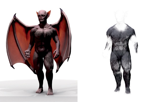
For the body layer, I enabled an ambient occlusion pass under Passes in the Layers panel. The result when rendered was two separate layers, as shown in Figure 14-4. When looking at the render (choose Render Result from the image selector drop-down menu), you can switch between these layers using the drop-down menu in the header of the UV Image editor.
In the Layers panel, the options and settings you choose apply only to the currently selected render layer. In other panels of the Render tab, options apply across all render layers. I set the Alpha option in the Shading panel to Straight Alpha and turned off Ray Tracing to speed up renders. (I didn’t need to use ray tracing since I was using buffered shadows for my spot lamps and approximate ambient occlusion.) I set the render size to 2200×3000 pixels in the Dimensions panel, and pressed Render (F12) to start rendering.
Compositing the Passes
After rendering, I used Blender’s compositor to combine the layers. I wanted to achieve certain effects with the compositor, in the following order:
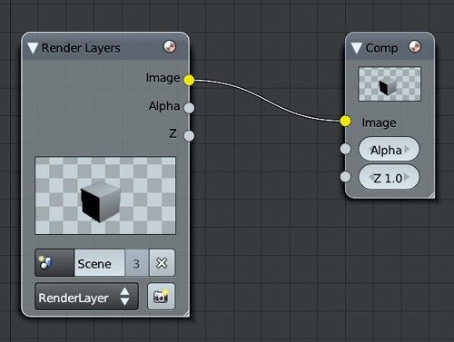
These effects (as with all things in the compositor) need to be applied in a particular order. Because each node is processed in the order it is connected, changing the order in which you apply nodes to your image can make a big difference. To begin compositing, make sure that Use Nodes is enabled and that you are editing the compositing nodes (not a material or texture). The default compositing node tree should look like Figure 14-5.
The initial Render node will use the first render layer you created in the Layers panel, which in my case was the body layer. I added a second Render Layer node (SHIFT-A▸Input▸Render Layer) to hold my strand render layer, selecting it from the drop-down menu at the bottom of the Render Layer node.
Extra Ambient Occlusion
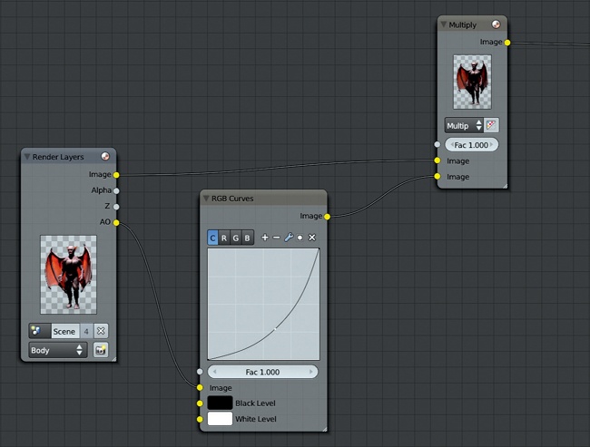
Next, I used a Mix node (SHIFT-A▸Color▸Mix) to increase the strength of the ambient occlusion effect on the body render layer. I set the Blend mode of the Mix node to Multiply and used the Image output of the body render layer as the first input. I used the ambient occlusion pass (from the socket labeled AO) as the second input.
To increase the effect, I darkened the ambient occlusion pass with a Curves node before multiplying it with the image. To do so, I added an RGB Curves node and inserted it between the ambient occlusion output of the Render Layer node and the Multiply node. To do this quickly, drag the node over the connection between two other nodes (you should see the connection highlight) and release it to insert it in a chain between the other two nodes.
Finally, I made the curve on the RGB Curves node a bit steeper (see Figure 14-6).
Combining the Body and Fur
Next, I added an Alpha Over node (SHIFT-A▸Color▸Alpha Over), connecting the body as the first input and the fur as the second. To get the correct results when compositing layers with straight alpha, which I selected when choosing the Render settings earlier (see Render Layers), I enabled Convert Premultiply for this node. This should produce the expected result without any dark fringing.
To place the Bat Creature on a dark gray background, I used a second Alpha node with an RGB node as the first input (set to gray) and my newly merged body and hair layers as the second input, as shown in Figure 14-6.
Bloom
Next, I added some bloom. Bloom is a common effect in both real and CG imagery, where light bleeds out from bright areas into darker ones, effectively lightening the image around darker areas. The real-world effect arises from imperfections in lenses, but I could mimic this by blurring my image and overlaying it on the original input.
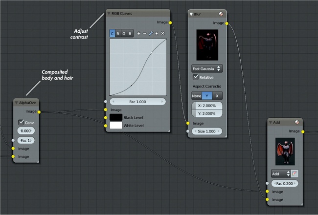
To generate bloom, I created a Blur node (SHIFT-A▸Filter▸Blur) and set its type to Fast Gaussian. I also enabled the Relative option, which would allow me to specify the blur radius relative to the width of the image. This option is useful if you don’t know what final resolution you want to use for your render, because the amount of blurring won’t appear to change if you make the render smaller or larger. (It would if you defined the radius in pixels.)
I set the x and y radii to 2 percent and selected Y under Aspect Correction to make sure the blur had the correct aspect ratio. (This applies only when using relative blur.) Then, I used an Add node with a factor of 0.2 to subtly add the result of the blurred image on top of the original.
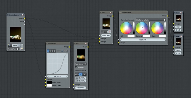
The initial effect was too bright, so I used another RGB Curves node to darken the darker regions of the image before it was blurred so that only the brightest regions would contribute to the bloom. The resulting node tree is shown in Figure 14-7.
Color Correction
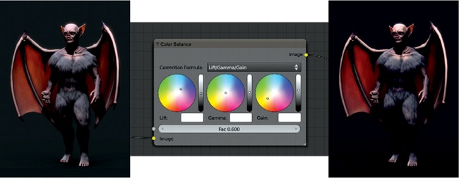
Next, I applied some basic color correction using the Color Balance node. This node is really useful for applying a range of color-grading effects to your renders. First, I added the Color Balance node. Then, I connected my composite-in-progress to its image input and turned the factor down to 0.6. (The Color Balance node can produce a strong effect, so turning the factor down is an easy way to make it more subtle without having to make very small adjustments to the other controls.)
The Color Balance node has three sets of controls, each of which sets an RGB color. You can set each input by using the color wheel to control the hue and saturation and using the vertical slider to control the color. The color you select is shown below in the color picker. You can also click the color picker to use Blender’s default color picker or to set RGB or HSV values manually.
The Color Balance node inputs are named lift, gamma, and gain, and they can be thought of as affecting the shadows, midtones, and highlights of an image. Thus, to give an image less prominent highlights, you could turn down the brightness of the lift input. To give it saturated red highlights, you could set the gain color toward red. In general, setting opposing colors for the lift and gain inputs often results in an image with nice color harmonies between the lights and darks.
In many Hollywood movies, the shadows are teal or blue, while the midtones and highlights are pushed toward orange—a color scheme that works well with the pinkish-orange of most lighter skin tones. For the Bat Creature, I opted for a slightly blue lift color and a slightly yellow gain color. The effect is shown in Figure 14-8.
Adding a Vignette
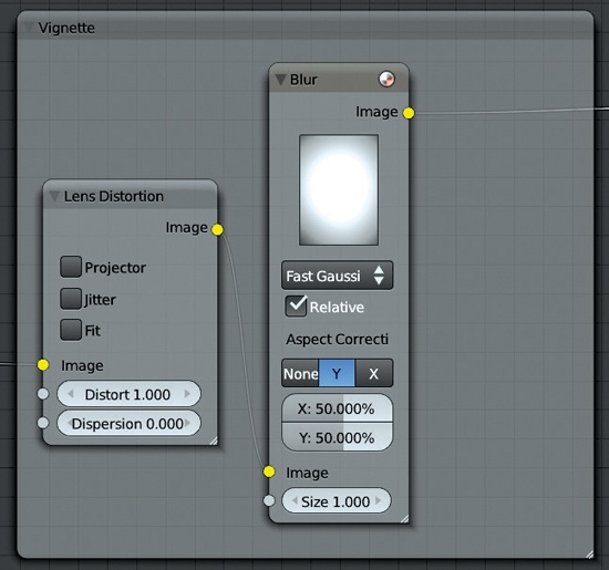
Next, I added a vignette to my image to slightly darken its corners and draw the viewer’s attention to the center of the frame. To create this effect, I took the alpha channel of my body layer and ran it thought a lens distortion filter with a distort value of 1. This distorted the image into a circular shape with black corners, which was almost what I needed.
Then, I used a Blur node set to Fast Gaussian Blur with a relative radius of 50 percent to blur the output of the Lens Distortion node. This gave the image a soft gradient out from the middle, which I then overlaid onto the color-corrected render.
Finally, I added a Sharpen node with a very low Factor setting (around 0.05) to the end of the node tree and connected the output to the Composite node. The final node tree is shown in Figure 14-9, and the result is shown in Figure 14-10.
Compositing Feedback and Viewer Nodes
Creating a final composite from your renders can be a long process that requires some experimentation. To aid in the process, Blender automatically recomposites your final render when you change the node tree. An alternative way to get a feel for how your node setup is working is to use the Viewer node, a secondary output node that lets you view any stage in your node tree.


To create a Viewer node, press SHIFT-A▸Output▸Viewer in the Node editor. Whatever is connected as the input for this node will then show up in the UV Image editor if you select Viewer Node from the drop-down menu or check Backdrop in the background of the Node editor header.
To quickly change which node the Viewer node is connected to, SHIFT-click any node in your setup. This allows you to easily go through your node tree, SHIFT-clicking each node in turn to see how it affects the composite. (You could create multiple Viewer nodes, but this method keeps your node tree clean.)
Organizing Node Trees with Frames and Node Groups
Node setups for compositing can become quite complex as you add more and more nodes. If you don’t keep them organized, it can be difficult to come back later to determine what’s going on in your node tree. To help with this, Blender lets you organize nodes as Frame nodes and node groups.
Frame Nodes
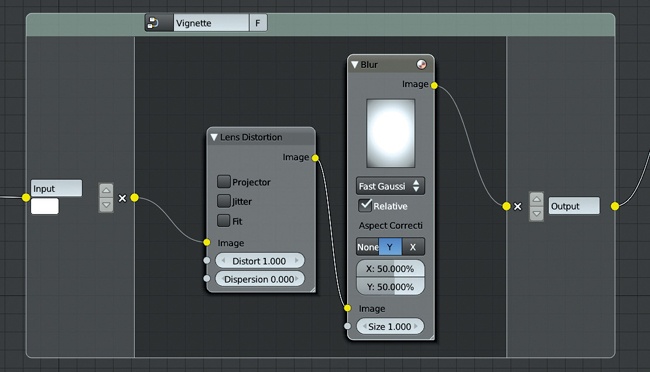
Frames are large, rectangular nodes with no inputs or outputs of their own; you place other nodes on top of them, which then “stick” to the frame node, allowing you to move collections of nodes together as one. You can label Frame nodes to mark the parts of your node setup (see Figure 14-11) by editing the node’s name in the Properties region (N). To unstick a node from a frame, you can use the shortcut ALT-P, or you can use ALT-F to unstick the node and automatically grab it to move it around.
Node Groups
Node groups are different from frames. To create a node group, select one or more nodes and press CTRL-G to group them into a single node. The new Group node should contain all of the selected nodes with the inputs and outputs required by the group as sockets. You can expand the group and look inside with TAB to modify its nodes and add extra inputs and outputs.
When you expand a node group, its inputs and outputs will be shown on the left and right sides of the group respectively (see Figure 14-12). To add an input or output, drag a connection from one of the nodes in the group to this border; to remove a connection, click the X next to it. Use the arrows next to each input or output to reorder them and tidy up the group.
Like all nodes, node groups can be duplicated and reused. Once duplicated, they behave like linked duplicate objects: A change within one instance of the group affects all instances the same way, which means that you can group commonly repeated chains of nodes and edit them all at once. Node groups can also be linked or appended from other .blend files, allowing you to reuse parts of your existing compositing setups.
Retouching in GIMP
Once you’re happy with your composite, you can call it final and save it as an image. Formats like PNG, TIFF, and Targa are good for this, being lossless formats (for saving images without losing quality). For posting to the Web, you may want to use the JPEG format, which compresses images much more, giving you a small file at the expense of a small loss in image quality. For the Bat Creature, though, I opted to fix some things in GIMP before calling it final. I wanted to soften some of the specular highlights on the nails and lighten the eyes a bit. I saved it as a Targa (.tga) file (F3 in the UV Image editor) and opened it in GIMP.
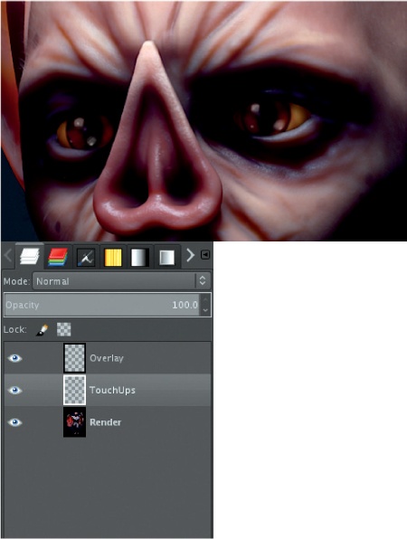
To lighten the eyes, I created a new layer and set its Blend mode to Overlay. Then, I painted white over the eyes. I also added subtle highlights, painting some distorted reflections by hand on a separate layer (this time with the Blend mode set to Normal).
On the same layer as the reflections, I also darkened the highlights on some of the nails, picking colors from nearby areas with the color picker and painting over the bright highlights. (Make sure to turn on Sample Merged in the tool options to allow you to sample layers below the current one without switching to them.) Finally, on the original render layer, I used the Blur tool to slightly blur some of the hair on the feet in order to draw attention away from where it looked a bit too coarse.
In Figure 14-13, you can see the retouched eyes. Figure 14-14 shows the completed Bat Creature project.
Rendering and Compositing the Spider Bot
To finalize the Spider Bot, I wanted to add color grading to the lighting (from Chapter 13), show some depth of field to communicate the robot’s small scale, and add some bloom.
Depth of field is a real-world phenomenon that happens with images seen through a lens, whether that’s a camera or the human eye. Lenses can only focus perfectly on objects that are a certain distance away from them, a distance known as the focal length. Objects outside this distance become progressively more out of focus. The effect can be subtle (even not worth bothering with) or significant. In general, depth-of-field effects are most apparent when viewing objects at small scales.
Depth of Field in Cycles
There are two ways to create depth of field when rendering with Cycles. One is to use the Defocus node in Blender’s compositor. This works with both Blender Internal and Cycles and will be used for the Jungle Temple scene later in this chapter. The other way is to use Cycles’s “real” depth of field as a Camera setting when rendering.
To use real depth of field, do the following:
Select the active camera.
In the Depth of Field panel on the Object Data tab of the Properties editor, set a distance from the camera to the focal plane (the distance where objects appear in focus).
Set an aperture size to determine the amount of blurring. This can be specified in terms of either a radius or a number of F/Stops. Higher numbers give more blur with radius or less with F/Stops. For the Spider Bot, I used radius to set the depth of field to about 0.3.
Note
Cycles can also mimic the shape of an aperture like the one you might find on a real film or digital camera. To do this, set Blades to the number of sides of the aperture shape and set Rotation to rotate the shape.
When setting the distance for the depth of field, you can either set a number manually with the Depth setting or specify an object using the selector under Focus. This causes the camera to ignore the Manual Depth setting and focus on the object’s center instead. It’s usually easiest to create an empty object, place it where you want the scene to be in focus, and then set this empty object as the depth-of-field target in the Camera settings.
To better visualize the depth-of-field distance, enable the Limits option in the Display panel of the Camera settings. Blender then displays a line pointing out from the camera (describing the clipping distances) with a yellow cross at the depth-of-field distance.
Render Settings for the Spider Bot
With depth of field set up, I was ready to render. I set the resolution of the render to 2600×3600, and in the Integrator panel of the Render tab, I set Render Samples to 1000 and Clamp to 2 to reduce the number of fireflies in the scene.
I wanted light to bounce around my scene and illuminate the shadows, but almost all of the scene is in direct light, so I didn’t need to rely on bounced light too heavily. I set Max Bounces to 32 (with a minimum of 4 to allow early termination) and the three Light Paths settings to 32 as well. I didn’t need any render layers or extra passes, so I left the Layers panel alone and pressed Render (F12).
Compositing the Spider Bot
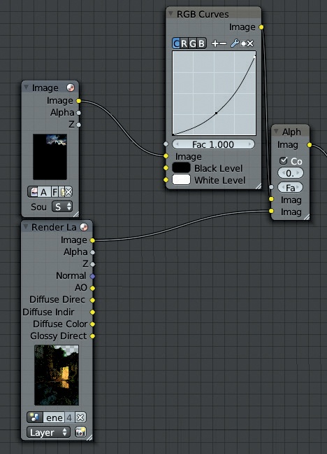
Next, I added some color grading and bloom to my final render. While Cycles provides some different render passes, the process of compositing is essentially the same as when using Blender Internal. I added bloom as I did with the Bat Creature, using a Blur node to blur the image and an Add node to add the result back onto the image. Again, I added an RGB Curves node before the Blur node to increase the contrast and slightly darken the image to be blurred.
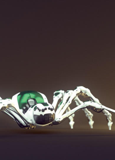
For color grading, I added a Color Balance node: I chose a purplish color for the Lift Color and a greenish tint for the Gain. I set the Gamma to slightly bluish and brightened up the highlights of the image a bit by setting the value of the gain slightly higher than 1.0. (You can set numerical values for the RGB or HSV colors for Lift, Gamma, and Gain by clicking the color picker.) I then connected the output of the Color Balance node to the image socket Composite output node. The finished node tree is shown in Figure 14-15 and the resulting composite in Figure 14-16.
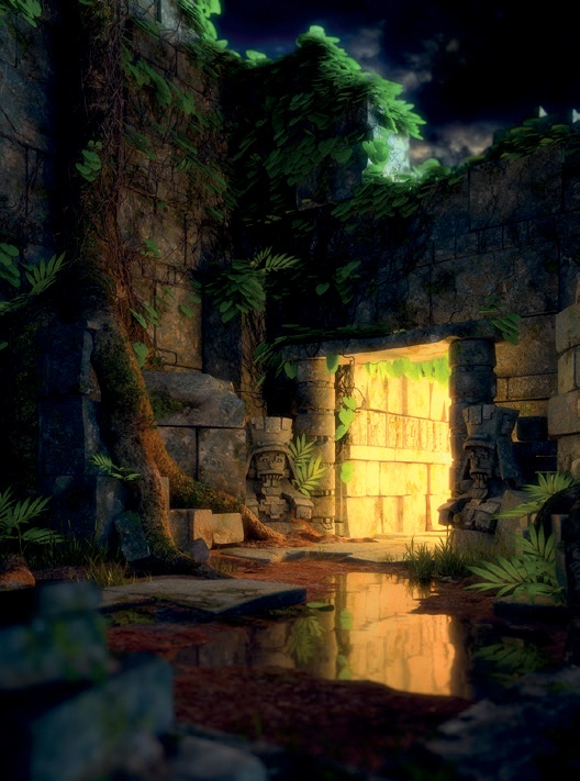
Rendering and Compositing the Jungle Temple
The Jungle Temple was a complex scene, and my Render settings had a much greater impact on render times for this project. I set the render size of the image to 2880×3840; the number of Render Samples in the Sampling settings to 5000; and Clamp to 3.0 to try to reduce noise a bit more quickly.
Note
Although 5000 samples is a lot, I wasn’t particularly concerned about how long my render took. Primarily, this high number was necessary because there were a lot of soft shadows in the scene. For good results with fewer samples, you can try turning down the Size setting on some of the lamps in your scene at the cost of harder-edged shadows.
For bounces, I set the Max to 128 and Min to 8 to allow for probabilistic ray termination. Because I wanted to composite the final render on a background image of clouds and sky, I turned on Transparent under Film options.
I left the other Render options at their default and pressed F12 to render.
Background Required
When compositing the Jungle Temple, I wanted to add bloom, depth of field, and some color grading. But first I needed to composite my render over a background, which meant creating a background in GIMP and then importing it into Blender with an Image Texture node for further compositing.
Painting the Sky in GIMP
To create a sky background, I first saved my uncomposited render from Blender’s Image editor as a .png image with transparency (when saving, remember to choose RGBA next to the file type to save the transparency as well). Then, I opened the image in GIMP. To create a background for the top right-hand corner, I opened a sky texture from CGTextures as a layer (see Figure 14-17) and put it below the render in my layer stack. I then scaled and positioned the background to put a nice bit of cloud in the top corner (as you can see in the first image in Figure 14-17). To create a nighttime background, I used the Curves tool to really darken the clouds layer, while using the Hue-Saturation and Brightness tools (Colors▸Hue-Saturation) to reduce the saturation of the layer a bit so that the colors didn’t look too saturated.
Next, I added some embellishments to the cloud image using the Dodge/Burn tool (set to Dodge) and added highlights to the edges of some clouds using a soft-edged brush. I also created a new transparent layer and set its Blend mode to Overlay. I then used this new layer to incorporate some extra colors around the clouds: a light blue around the edges of the leaves on the temple and some greens and yellows toward the corner. Throughout, my goal was to end up with a background that had a color palette similar to that of my rendered image.
Finally, I hid the render layer, saved the background on its own as an .xcf file (CTRL-S) so that I could edit it later, and exported it as a .tga image (CTRL-E). The background image and its various stages are shown in Figure 14-17.
Compositing the Temple
With my background created, I returned to Blender’s compositor. First, I had to add my background behind my render. To do so, I used the Alpha Over node with the background as the first input and my render as the second (see Figure 14-18).

Depth of Field
Next came some depth of field. When adding depth of field to the Spider Bot, I used physically correct, rendered depth of field. However, for the Jungle Scene, I used the compositor’s Defocus node. This method gives slightly less accurate results than rendered depth of field, but it allows for more control over which areas are blurred and which are not and lets us change the focus after we finish rendering, which gives us more flexibility.
The Defocus node requires two inputs: the image to be blurred and a black-and-white mask that determines how much to blur different parts of the image. For the mask, you can use either the z-buffer directly (check the Use z-buffer input checkbox), or you can use any black-and-white image as a simple mask by leaving it unchecked. If you choose to use the z-buffer directly, Blender will use the camera’s depth-of-field settings found in the Object Data tab of the Properties editor. Regions closer or farther than the depth-of-field distance will be blurred. If you turn this option off, Blender will use the value of the input to determine the amount of blurring so that white regions will be the most blurred and black the least.
For the Jungle Temple scene, I opted to use the z-buffer directly, but I added a Blur node (with a radius of 6 pixels) between the z-buffer output and the z-input of the Defocus node to blur these values slightly. This method reduces the creation of artifacts on foreground objects, where objects that should be blurred appear to have sharp edges.
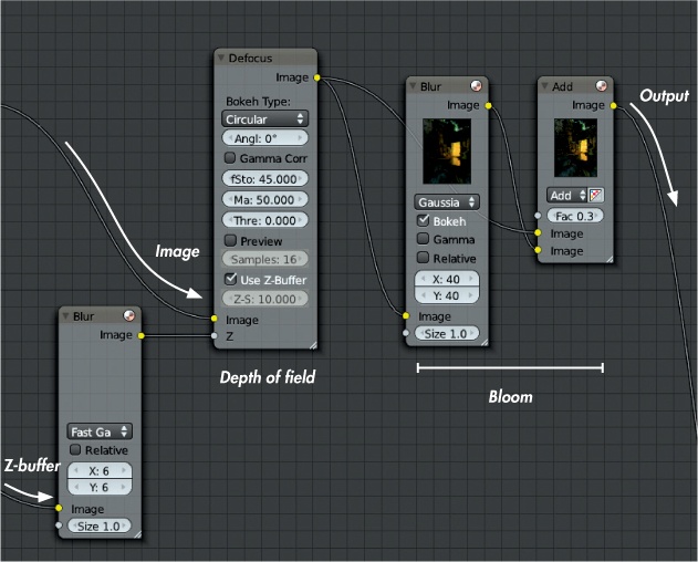
Adding Bloom and Vignetting
Next, I added some bloom. As with the other projects, I blurred the image and combined it back over the image with an Add Mix node. I applied some vignetting by taking the alpha channel of the render, distorting it with the Lens Distortion node, blurring it with the Blur node, and then overlaying this on top of the image. The nodes for these stages are shown in Figure 14-19.
Color Grading
To add color grading, I used two different nodes. First, I put the image through a Hue Correct node, which let me adjust the saturation (or hue or value) of specific colors within the image. Because I wanted to play up the oranges and greens before applying some extra grading, I adjusted the curve of the Hue Correct node by clicking the curve and dragging to add a new point, raising the profile of the curve in the orange and green areas, and lowering it slightly in the blues. This increased the saturation of the orange light from the temple entrance and the green of the leaves, making them more prominent. I ran the result through a Color Balance node, adding some blues to the shadows with a bluish lift color and some yellow and orange to the midtones and highlights with very slightly orange gamma and gain colors.
Finally, I added a Filter node at the end of the node tree, just before the Composite output node. I set this to Sharpen with a factor of 0.05 to add some very slight sharpening to the image.
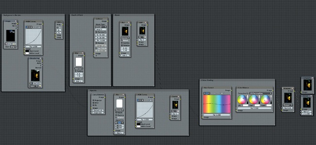
This completes the compositing for the Jungle Temple scene. The complete node setup is shown in Figure 14-20.
As a final adjustment, I opened the composite image in GIMP and cleaned up one or two remaining depth-of-field artifacts by hand with the Blur tool. I also cropped the image slightly to improve the composition. The result is shown in Figure 14-21.
In Review
This more or less completes each of the projects I set out to create for the book. In this chapter, I took the final scenes and rendered them using either Cycles or Blender Internal as render engines. Then I took the render output and used GIMP and Blender’s compositor to tweak and refine these results into my final images. The result is renders of the projects that I can now call finished.
Of course, there’s always another tweak that can be made, and in Chapter 15, we’ll look at a few more things that could be done with these projects to take them further.