This chapter includes a discussion of the fundamental concepts that influence the displacement of oil and gas both by internal displacement processes and by external flooding processes. It is meant to be an introduction to these topics and not an exhaustive treatise. The reader, if interested, is referred to other works that cover the material in this chapter.1–5 The reservoir engineer should be exposed to these concepts because they form the basis for understanding secondary and tertiary flooding techniques, discussed in the next chapter, as well as some primary recovery mechanisms.
The overall recovery efficiency E of any fluid displacement process is given by the product of the macroscopic, or volumetric displacement, efficiency, Ev, and the microscopic displacement efficiency, Ed:
The macroscopic displacement efficiency is a measure of how well the displacing fluid has contacted the oil-bearing parts of the reservoir. The microscopic displacement efficiency is a measure of how well the displacing fluid mobilizes the residual oil once the fluid has contacted the oil.
The macroscopic displacement efficiency is made up of two other terms: the areal, Es, sweep efficiency and the vertical, Ei, sweep efficiency.
The microscopic displacement efficiency is affected by the following factors: interfacial and surface tension forces, wettability, capillary pressure, and relative permeability.
When a drop of one immiscible fluid is immersed in another fluid and comes to rest on a solid surface, the surface area of the drop will take a minimum value owing to the forces acting at the fluid-fluid and rock-fluid interfaces. The forces per unit length acting at the fluid-fluid and rock-fluid interfaces are referred to as interfacial tensions. The interfacial tension between two fluids represents the amount of work required to create a new unit of surface area at the interface. The interfacial tension can also be thought of as a measure of the immiscibility of two fluids. Typical values of oil-brine interfacial tensions are on the order of 20 dynes/cm to 30 dynes/cm. When certain chemical agents are added to an oil-brine system, it is possible to reduce the interfacial tension by several orders of magnitude.
The tendency for a solid to prefer one fluid over another is called wettability. Wettability is a function of the chemical composition of both the fluids and the rock. Surfaces can be either oil wet or water wet, depending on the chemical composition of the fluids. The degree to which a rock is either oil wet or water wet is strongly affected by the absorption or desorption of constituents in the oil phase. Large, polar compounds in the oil phase can absorb onto the solid surface, leaving an oil film that may alter the wettability of the surface.
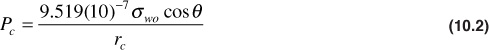
The concept of wettability leads to another significant factor in the recovery of oil. This factor is capillary pressure. To illustrate capillary pressure, consider a capillary tube that contains both oil and brine, the oil having a lower density than the brine. The pressure in the oil phase immediately above the oil-brine interface in the capillary tube will be slightly greater than the pressure in the water phase just below the interface. This difference in pressure is called the capillary pressure, Pc, of the system. The greater pressure will always occur in the nonwetting phase. An expression relating the contact angle, θ; the radius, rc, of the capillary in feet; the oil-brine interfacial tension, σwo, in dynes/cm; and the capillary pressure in psi is given by
This equation suggests that the capillary pressure in a porous medium is a function of the chemical composition of the rock and fluids, the pore-size distribution of the sand grains in the rock, and the saturation of the fluids in the pores. Capillary pressures have also been found to be a function of the saturation history, although this dependence is not reflected in Eq. (10.2). For this reason, different values of capillary pressure are obtained during the drainage process (i.e., displacing the wetting phase by the nonwetting phase), then during the imbibitions process (i.e., displacing the nonwetting phase with the wetting phase). This hysteresis phenomenon is exhibited in all rock-fluid systems.
It has been shown that the pressure required to force a nonwetting phase through a small capillary can be very large. For instance, the pressure drop required to force an oil drop through a tapering constriction that has a forward radius of 0.00002 ft, a rearward radius of 0.00005 ft, a contact angle of 0°, and an interfacial tension of 25 dynes/cm is 0.71 psi. If the oil drop were 0.00035-ft long, a pressure gradient of 2029 psi/ft would be required to move the drop through the constriction. Pressure gradients of this magnitude are not realizable in reservoirs. Typical pressure gradients obtained in reservoir systems are of the order of 1 psi/ft to 2 psi/ft.
Another factor affecting the microscopic displacement efficiency is the fact that when two or more fluid phases are present and flowing, the saturation of one phase affects the permeability of the other(s). The next section discusses in detail the important concept of relative permeability.
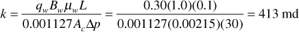
Except for gases at low pressures, the permeability of a rock is a property of the rock and not of the fluid that flows through it, provided that the fluid saturates 100% of the pore space of the rock. This permeability at 100% saturation of a single fluid is called the absolute permeability of the rock. If a core sample 0.00215 ft2 in cross section and 0.1-ft long flows a 1.0 cp brine with a formation volume factor of 1.0 bbl/STB at the rate of 0.30 STB/day under a 30 psi pressure differential, it has an absolute permeability of
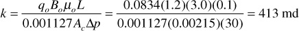
If the water is replaced by an oil of 3.0-cp viscosity and 1.2-bbl/STB formation volume factor, then, under the same pressure differential, the flow rate will be 0.0834 STB/day, and again the absolute permeability is
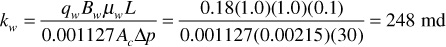
If the same core is maintained at 70% water saturation (Sw = 70%) and 30% oil saturation (So = 30%), and at these and only these saturations and under the same pressure drop, it flows 0.18 STB/day of the brine and 0.01 STB/day of the oil, then the effective permeability to water is
and the effective permeability to oil is
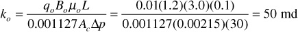
The effective permeability, then, is the permeability of a rock to a particular fluid when that fluid has a pore saturation of less than 100%. As noted in the foregoing example, the sum of the effective permeabilities (i.e., 298 md) is always less than the absolute permeability, 413 md.
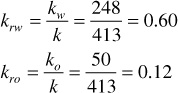
When two fluids, such as oil and water, are present, their relative rates of flow are determined by their relative viscosities, their relative formation volume factors, and their relative permeabilities. Relative permeability is the ratio of effective permeability to the absolute permeability. For the previous example, the relative permeabilities to water and to oil are
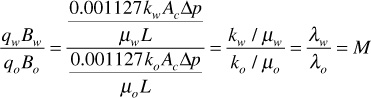
The flowing water-oil ratio at reservoir conditions depends on the viscosity ratio and the effective permeability ratio (i.e., on the mobility ratio), or
For the previous example,
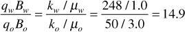
At 70% water saturation and 30% oil saturation, the water is flowing at 14.9 times the oil rate. Relative permeabilities may be substituted for effective permeabilities in the previous calculation because the relative permeability ratio, krw/kro, equals the effective permeability ratio, kw/ko. The term relative permeability ratio is more commonly used. For the previous example,
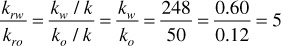
Water flows at 14.9 times the oil rate because of a viscosity ratio of 3 and a relative permeability ratio of 5, both of which favor the water flow. Although the relative permeability ratio varies with the water-oil saturation ratio—in this example 70/30, or 2.33—the relationship is unfortunately far from one of simple proportionality.
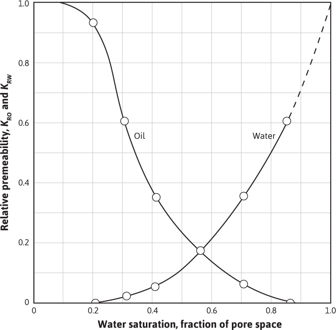
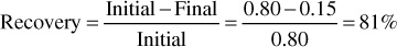
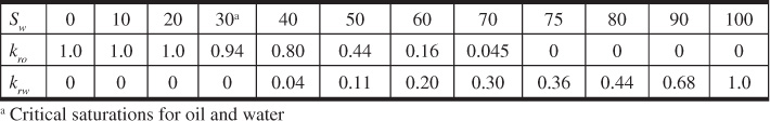
Figure 10.1 shows a typical plot of oil and water relative permeability curves for a particular rock as a function of water saturation. Starting at 100% water saturation, the curves show that a decrease in water saturation to 85% (a 15% increase in oil saturation) sharply reduces the relative permeability to water from 100% down to 60%, and at 15% oil saturation, the relative permeability to oil is essentially zero. This value of oil saturation, 15% in this case, is called the critical saturation, the saturation at which oil first begins to flow as the oil saturation increases. It is also called the residual saturation, the value below which the oil saturation cannot be reduced in an oil-water system. This explains why oil recovery by water drive is not 100% efficient. If the initial connate water saturation is 20% for this particular rock, then the maximum recovery from the portion of the reservoir invaded by high-pressure water influx is
Experiments show that essentially the same relative permeability curves are obtained for a gas-water system as for the oil-water system, which also means that the critical, or residual, gas saturation will be the same. Furthermore, it has been found that if both oil and free gas are present, the residual hydrocarbon saturation (oil and gas) will be about the same, in this case 15%. Suppose, then, that the rock is invaded by water at a pressure below saturation pressure so that gas has evolved from the oil phase and is present as free gas. If, for example, the residual free gas saturation behind the flood front is 10%, then the oil saturation is 5%, and neglecting small changes in the formation volume factors of the oil, the recovery is increased to
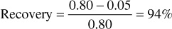
The recovery, of course, would not include the amount of free gas that once was part of the initial oil phase and has come out of solution.
Returning to Fig. 10.1, as the water saturation decreases further, the relative permeability to water continues to decrease and the relative permeability to oil increases. At 20% water saturation, the (connate) water is immobile, and the relative permeability to oil is quite high. This explains why some rocks may contain as much as 50% connate water and yet produce water-free oil. Most reservoir rocks are preferentially water wet—that is, the water phase and not the oil phase is next to the walls of the pore spaces. Because of this, at 20% water saturation, the water occupies the least favorable portions of the pore spaces—that is, as thin layers about the sand grains, as thin layers on the walls of the pore cavities, and in the smaller crevices and capillaries. The oil, which occupies 80% of the pore space, is in the most favorable portions of the pore spaces, which is indicated by a relative permeability of 93%. The curves further indicate that about 10% of the pore spaces contribute nothing to the permeability, for at 10% water saturation, the relative permeability to oil is essentially 100%. Conversely, on the other end of the curves, 15% of the pore spaces contribute 40% of the permeability, for an increase in oil saturation from zero to 15% reduces the relative permeability to water from 100% to 60%.
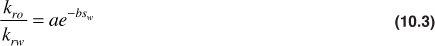
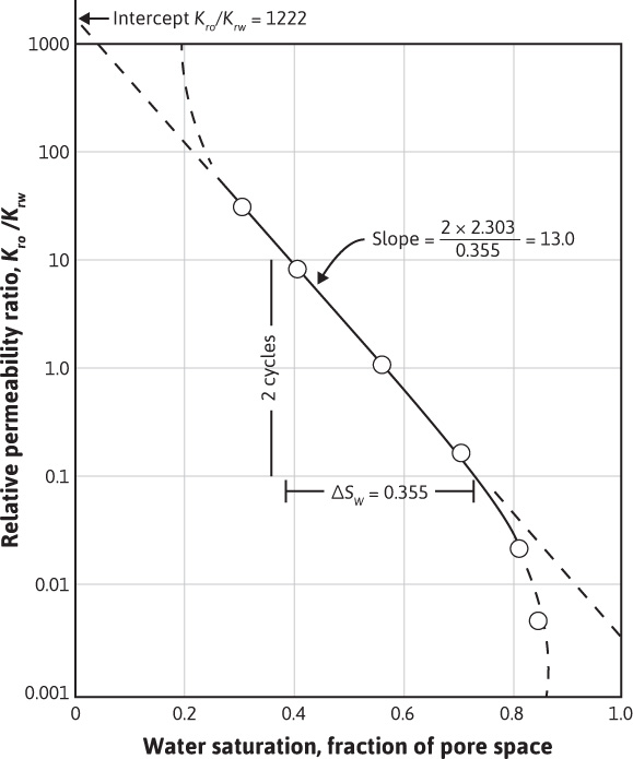
In describing two-phase flow mathematically, it is typically the relative permeability ratio that enters the equations. Figure 10.2 is a plot of the relative permeability ratio versus water saturation for the same data of Fig. 10.1. Because of the wide range of kro/krw values, the relative permeability ratio is usually plotted on the log scale of a semilog graph. The central or main portion of the curve is quite linear on the semilog plot and in this portion of the curve, the relative permeability ratio may be expressed as a function of the water saturation by
The constants a and b may be determined from the graph shown in Fig. 10.2, or they may be determined from simultaneous equations. At Sw = 0.30, kro/krw = 25, and at Sw = 0.70, kro/krw = 0.14. Then,
25 = ae–0.30b and 0.14 = ae –0.70b
Solving simultaneously, the intercept a = 1220 and the slope b = 13.0. Equation (10.3) indicates that the relative permeability ratio for a rock is a function of only the relative saturations of the fluids present. Although it is true that the viscosities, the interfacial tensions, and other factors have some effect on the relative permeability ratio, for a given rock, it is mainly a function of the fluid saturations.
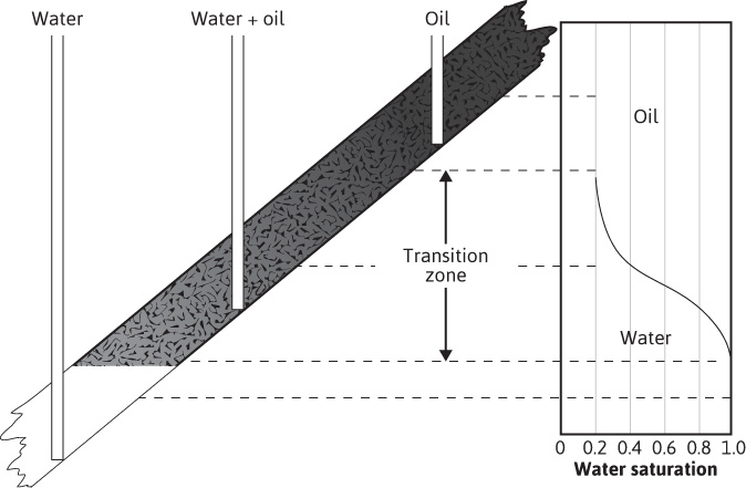
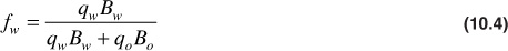
In many rocks, there is a transition zone between the water and the oil zones. In the true water zone, the water saturation is essentially 100%, although in some reservoirs, a small oil saturation may be found a considerable distance vertically below the oil-water contact. In the oil zone, there is usually connate water present, which is essentially immobile. For the present example, the connate water saturation is 20% and the oil saturation is 80%. Only water will be produced from a well completed in the true water zone, and only oil will be produced from the true oil zone. In the transition zone (Fig. 10.3), both oil and water will be produced, and the fraction that is water will depend on the oil and water saturations at the point of completion. If the well in Fig. 10.3 is completed in a uniform sand at a point where So = 60% and Sw = 40%, the fraction of water in reservoir flow rate units or reservoir watercut may be calculated using Eq. (8.19):
Since watercut, fw, is defined as
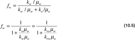
Combining these equations and canceling common terms,
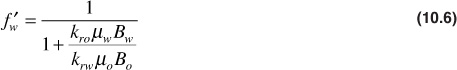
The fractional flow in surface flow rate units, or surface watercut, may be expressed as
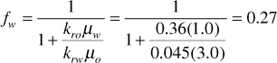
Either Eq. (10.5) or (10.6) can be used with the data of Fig. 10.1 and with viscosity data to calculate the watercut. From Fig. 10.1, at Sw = 0.40, krw = 0.045, and kro = 0.36. If μw = 1.0 cp and μo = 3.0 cp, then the reservoir watercut is
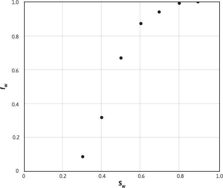
If the calculations for the reservoir watercut are repeated at several water saturations, and then the calculated values plotted versus water saturation, Fig. 10.4 will be the result. This plot is referred to as the fractional flow curve. The curve shows that the fractional flow of water ranges from 0 (for Sw≤ the connate water saturation) to 1 (for Sw ≥ 1 minus the residual oil saturation).
Figure 10.4 Fractional flow curve for the relative permeability data of Figure 10.1.
The following factors affect the macroscopic displacement efficiency: heterogeneities and anisotropy, mobility of the displacing fluids compared with the mobility of the displaced fluids, the physical arrangement of injection and production wells, and the type of rock matrix in which the oil or gas exists.
Heterogeneities and anisotropy of a hydrocarbon-bearing formation have a significant effect on the macroscopic displacement efficiency. The movement of fluids through the reservoir will not be uniform if there are large variations in such properties as porosity, permeability, and clay cement. Limestone formations generally have wide fluctuations in porosity and permeability. Also, many formations have a system of microfractures or large macrofractures. Any time a fracture occurs in a reservoir, fluids will try to travel through the fracture because of the high permeability of the fracture, which may lead to substantial bypassing of hydrocarbon.
Many producing zones are variable in permeability, both vertically and horizontally, leading to reduced vertical, Ei, and areal, Es, sweep efficiencies. Zones or strata of higher or lower permeability often exhibit lateral continuity throughout a reservoir or a portion thereof. Where such permeability stratification exists, the displacing water sweeps faster through the more permeable zones so that much of the oil in the less permeable zones must be produced over a long period of time at high water-oil ratios. The situation is the same, whether the water comes from natural influx or from injection systems.
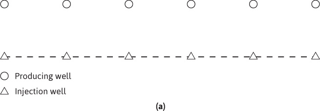
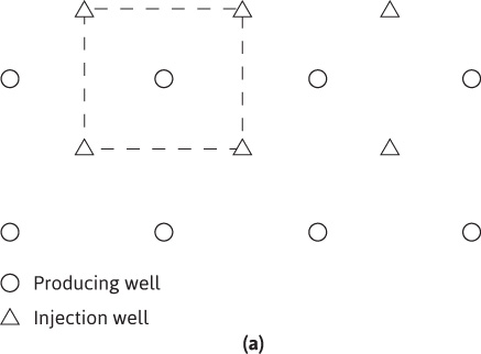
The areal sweep efficiency is also affected by the type of flow geometry in a reservoir system. As an example, linear displacement occurs in uniform beds of constant cross section, where the entire input and outflow ends are open to flow. Under these conditions, the flood front advances as a plane (neglecting gravitational forces), and when it breaks through at the producing end, the sweep efficiency is 100%—that is, 100% of the bed volume has been contacted by the displacing fluid. If the displacing and displaced fluids are injected into and produced from wells located at the input and outflow ends of a uniform linear bed, such as the direct line-drive pattern arrangement shown in Fig. 10.5(a), the flood front is not a plane, and at breakthrough, the sweep efficiency is far from 100%, as shown in Fig. 10.5(b).
Figure 10.5(b) The photographic history of a direct-line-drive fluid-injection system, under steady-state conditions, as obtained with a blotting-paper electrolytic model (after Wyckoff, Botset, and Muskat6).
Mobility is a relative measure of how easily a fluid moves through porous media. The apparent mobility, as defined in Chapter 8, is the ratio of effective permeability to fluid viscosity. Since the effective permeability is a function of fluid saturations, several apparent mobilities can be defined. When a fluid is being injected into a porous medium containing both the injected fluid and a second fluid, the apparent mobility of the displacing phase is usually measured at the average displacing phase saturation when the displacing phase just begins to break through at the production site. The apparent mobility of the nondisplacing phase is measured at the displacing phase saturation that occurs just before the beginning of the injection of the displacing phase.
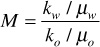
Areal sweep efficiencies are a strong function of the mobility ratio. The mobility ratio M, as defined in Chapter 8, is a measure of the relative apparent mobilities in a displacement process and is given by
A phenomenon called viscous fingering can take place if the mobility of the displacing phase is much greater than the mobility of the displaced phase. Viscous fingering simply refers to the penetration of the much more mobile displacing phase into the phase that is being displaced.
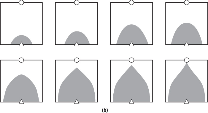
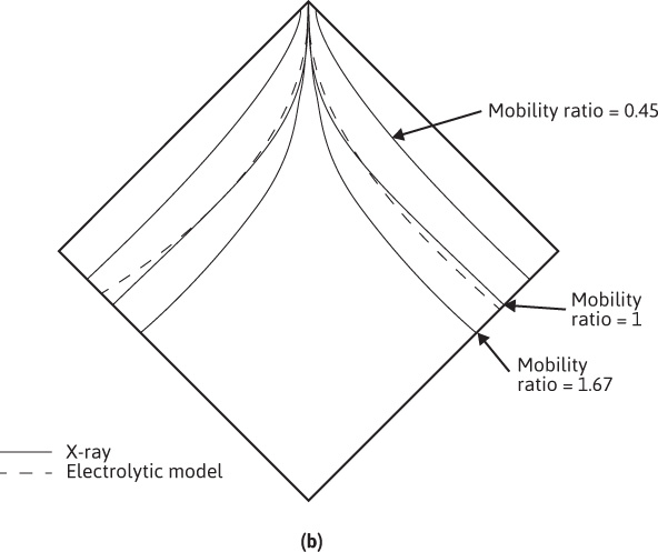
Figure 10.6(b) shows the effect of mobility ratio on areal sweep efficiency at initial breakthrough for a five-spot network (shown in Fig. 10.6(a)) obtained using the X-ray shadowgraph. The pattern at breakthrough for a mobility ratio of 1 obtained with an electrolytic model is included for comparison.
Figure 10.6(b) X-ray shadowgraph studies showing the effect of mobility ratio on areal sweep efficiency at breakthrough (after Slobod and Caudle7).
The arrangement of injection and production wells depends primarily on the geology of the formation and the size (areal extent) of the reservoir. For a given reservoir, an operator has the option of using the existing well arrangement or drilling new wells in other locations. If the operator opts to use the existing well arrangement, there may be a need to consider converting production wells to injection wells or vice versa. An operator should also recognize that, when a production well is converted to an injection well, the production capacity of the reservoir will have been reduced. This decision can often lead to major cost items in an overall project and should be given a great deal of consideration. Knowledge of any directional permeability effects and other heterogeneities can aid in the consideration of well arrangements. The presence of faults, fractures, and high-permeability streaks can dictate the shutting in of a well near one of these heterogeneities. Directional permeability trends can lead to a poor sweep efficiency in a developed pattern and can suggest that the pattern be altered in one direction or that a different pattern be used.
Sandstone formations are characterized by a more uniform pore geometry than limestone formations. Limestone formations have large holes (vugs) and can have significant fractures that are often connected. Limestone formations are associated with connate water that can have high levels of divalent ions such as Ca2+ and Mg2+. Vugular porosity and high-divalent ion content in their connate waters hinder the application of injection processes in limestone reservoirs. On the other hand, sometimes a sandstone formation can be composed of small sand grains that are so tightly packed that fluids will not readily flow through the formation.
Oil is displaced from a rock by water similar to how fluid is displaced from a cylinder by a leaky piston. Buckley and Leverett developed a theory of displacement based on the relative permeability concept.8 Their theory is presented here.
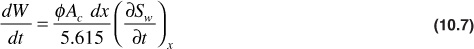
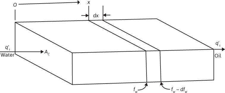
Consider a linear bed containing oil and water (Fig. 10.7). Let the total throughput, q′ = qwBw + qoBo, in reservoir barrels be the same at all cross sections. For the present, we will neglect gravitational and capillary forces that may be acting. Let Sw be the water saturation in any element at time t (days). Then if oil is being displaced from the element, at time (t + dt), the water saturation will be (Sw + dSw). If φ is the total porosity fraction, Ac is the cross section in square feet, and dx is the thickness of the element in feet, then the rate of increase of water in the element at time t in barrels per day is
The subscript x on the derivative indicates that this derivative is different for each element. If fw is the fraction of water in the total flow of  barrels per day, then
  is the rate of water entering the left-hand face of the element, dx. The oil saturation will be slightly higher at the right-hand face, so the fraction of water flowing there will be slightly less, or fw – dfw. Then the rate of water leaving the element is
  . The net rate of gain of water in the element at any time, then, is
Now, for a given rock, the fraction of water fw is a function only of the water saturation Sw, as indicated by Eq. (10.5), assuming constant oil and water viscosities. The water saturation, however, is a function of both time and position, x, which may be expressed as fw = F(Sw) and Sw = G(t, x). Then
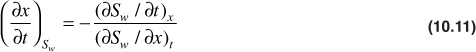
Now, there is interest in determining the rate of advance of a constant saturation plane, or front, (∂x/∂t)Sw (i.e., where Sw is constant). Then, from Eq. (10.10),
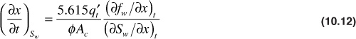
Substituting Eq. (10.9) in Eq. (10.11),
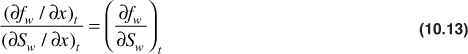
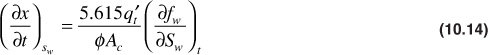
Eq. (10.12) then becomes
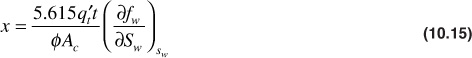
Because the porosity, area, and throughput are constant and because, for any value of Sw, the derivative ∂fw/∂Sw is a constant, the rate dx/dt is constant. This means that the distance a plane of constant saturation, Sw, advances is directly proportional to time and to the value of the derivative (∂fw/∂Sw) at that saturation, or
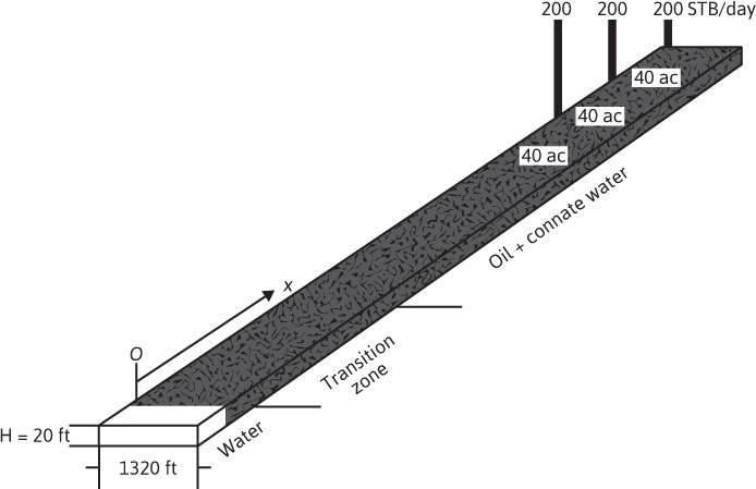
We now apply Eq. (10.15) to a reservoir under active water drive where the walls are located in uniform rows along the strike on 40-ac spacing, as shown in Fig. 10.8. This gives rise to approximate linear flow, and if the daily production of each of the three wells located along the dip is 200 STB of oil per day, then for an active water drive and an oil volume factor of 1.50 bbl/STB, the total reservoir throughput, will be 900 bbl/day.
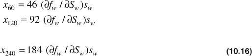
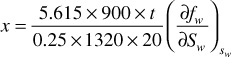
The cross-sectional area is the product of the width, 1320 ft, and the true formation thickness, 20 ft, so that for a porosity of 25%, Eq. (10.15) becomes
If we let x = 0 at the bottom of the transition zone, as indicated in Fig. 10.8, then the distances the various constant water saturation planes will travel in, say, 60, 120, and 240 days are given by
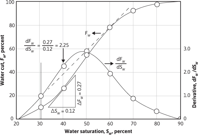
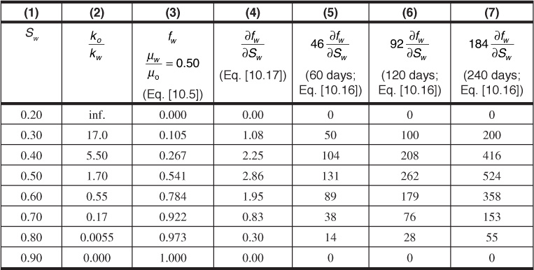
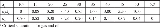
The value of the derivative (∂fw/∂Sw) may be obtained for any value of water saturation, Sw, by plotting fw from Eq. (10.5) versus Sw and graphically taking the slopes at values of Sw. This is shown in Fig. 10.9 at 40% water saturation, using the relative permeability ratio data of Table 10.1 and a water-oil viscosity ratio of 0.50. For example, at Sw = 0.40, where ko/kw = 5.50 (Table 10.1),
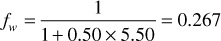
The slope taken graphically at Sw = 0.40 and fw = 0.267 is 2.25, as shown in Fig. 10.9.
The derivative (∂fw/∂Sw) may also be obtained mathematically using Eq. (10.3) to represent the relationship between the relative permeability ratio and the water saturation. Differentiating Eq. (10.16), the following is obtained:
For the ko/kw data of Table 10.1, a = 540 and b = 11.5. Then, at Sw = 0.40, for example, by Eq. (10.17),
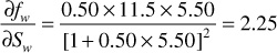
Figure 10.9 shows the fractional watercut, fW, and also the derivative (∂fw/∂Sw) plotted against water saturation from the data of Table 10.1. Equation (10.17) was used to determine the values of the derivative. Since Eq. (10.3) does not hold for the very high and for the quite low water saturation ranges, some error is introduced below 30% and above 80% water saturation. Since these are in the regions of the lower values of the derivatives, the overall effect on the calculation is small.
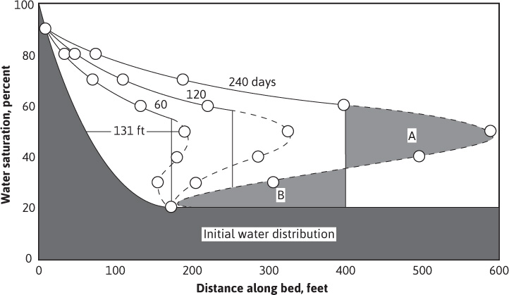
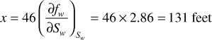
The lowermost curve of Fig. 10.10 represents the initial distribution of water and oil in the linear sand body of Fig. 10.8. Above the transition zone, the connate water saturation is constant at 20%. Equation (10.16) may be used with the values of the derivatives, calculated in Table 10.1 and plotted in Fig. 10.9, to construct the frontal advance curves shown in Fig. 10.10 at 60, 120, and 240 days. For example, at 50% water saturation, the value of the derivative is 2.86; so by Eq. (10.16), at 60 days, the 50% water saturation plane, or front, will advance a distance of
This distance is plotted as shown in Fig. 10.10 along with the other distances that have been calculated in Table 10.1 for the other time values and other water saturations. These curves are characteristically double valued or triple valued. For example, Fig. 10.10 indicates that the water saturation after 240 days at 400 ft is 20%, 36%, and 60%. The saturation can be only one value at any place and time. The difficulty is resolved by dropping perpendiculars so that the areas to the right (A) equal the areas to the left (B), as shown in Fig. 10.10.
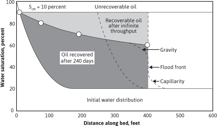
Figure 10.11 represents the initial water and oil distributions in the reservoir unit and also the distributions after 240 days, provided the flood front has not reached the lowermost well. The area to the right of the flood front in Fig. 10.11 is commonly called the oil bank and the area to the left is sometimes called the drag zone. The area above the 240-day curve and below the 90% water saturation curve represents oil that may yet be recovered or dragged out of the high-water saturation portion of the reservoir by flowing large volumes of water through it. The area above the 90% water saturation curve represents unrecoverable oil, since the critical oil saturation is 10%.
This presentation of the displacement mechanism has assumed that capillary and gravitational forces are negligible. These two forces account for the initial distribution of oil and water in the reservoir unit, and they also act to modify the sharp flood front in the manner indicated in Fig. 10.11. If production ceases after 240 days, the oil-water distribution will approach one similar to the initial distribution, as shown by the dashed curve in Fig. 10.11.
Figure 10.11 also indicates that a well in this reservoir unit will produce water-free oil until the flood front approaches the well. Thereafter, in a relatively short period, the watercut will rise sharply and be followed by a relatively long period of production at high, and increasingly higher, watercuts. For example, just behind the flood front at 240 days, the water saturation rises from 20% to about 60%—that is, the watercut rises from zero to 78.4% (see Table 10.1). When a producing formation consists of two or more rather definite strata, or stringers, of different permeabilities, the rates of advance in the separate strata will be proportional to their permeabilities, and the overall effect will be a combination of several separate displacements, such as described for a single homogeneous stratum.
The method discussed in the previous section also applies to the displacement of oil by gas drive. The treatment of oil displacement by gas in this section considers only gravity drainage along dip. Richardson and Blackwell showed that in some cases there can be a significant vertical component of drainage.9
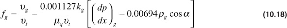
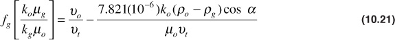
Due to the high oil-gas viscosity ratios and the high gas-oil relative permeability ratios at low gas saturations, the displacement efficiency by gas is generally much lower than that by water, unless the gas displacement is accompanied by substantial gravitational segregation. This is basically the same reason for the low recoveries from reservoirs produced under the dissolved gas drive mechanism. The effect of gravitational segregation in water-drive oil reservoirs is usually of much less concern because of the higher displacement efficiencies and the lower oil-water density differences, whereas the converse is generally true for gas-oil systems. Welge showed that capillary forces may generally be neglected in both, and he introduced a gravitational term in Eq. (10.5), as will be shown in the following equations.10 As with water displacement, a linear system is assumed, and a constant gas pressure throughout the system is also assumed so that a constant throughput rate may be used. These assumptions also allow us to eliminate changes caused by gas density, oil density, oil volume factor, and the like. Equation (8.1) may be applied to both the oil and gas flow, assuming the connate water is essentially immobile, so that the fraction of the flowing reservoir fluid volume, which is gas, is
The total velocity is vt, which is the total throughput rate divided by the cross-sectional area Ac. The reservoir gas density, ρg, is in lbm/ft3. The constant 0.00694 that appears in Eqs. (10.18) and (10.19) is a result of multiplying 0.433 and 62.4 lbm/ft3, the density of water. When capillary forces are neglected, as they are in this application, the pressure gradients in the oil and gas phases are equal. Equation (8.1) may be solved for the pressure gradient by applying it to the oil phase, or
Substituting the pressure gradient of Eq. (10.19) in Eq. (10.18),
Expanding and multiplying through by (ko/kg)(μg/μo),
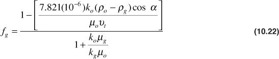
But νo/νt is the fraction of oil flowing, which equals 1 minus the gas flowing, (1 – fg). Then, finally,
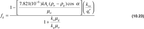
The relative permeability ratio (kro/krg) may be used for the effective permeability ratio in the denominator of Eq. (10.22); however, the permeability to oil, ko, in the numerator is the effective permeability and cannot be replaced by the relative permeability. It may, however, be replaced with (krok), where k is the absolute permeability. The total velocity, νt, is the total throughput rate, divided by the cross-sectional area, Ac. Inserting these equivalents, the fractional gas flow equation with gravitational segregation becomes
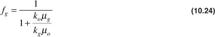
If the gravitational forces are small, Eq. (10.23) reduces to the same type of fractional flow equation as Eq. (10.5), or
Although Eq. (10.24) is not rate sensitive (i.e., it does not depend on the throughput rate), Eq. (10.23) includes the throughput velocity  and is therefore rate sensitive. Since the total throughput rate, , is in the denominator of the gravitational term of Eq. (10.23), rapid displacement (i.e., large
  ) reduces the size of the gravitational term, and so causes an increase in the fraction of gas flowing, fg. A large value of fg implies low displacement efficiency. If the gravitational term is sufficiently large, fg becomes zero, or even negative, which indicates countercurrent flow of gas updip and oil downdip, resulting in maximum displacement efficiency. In the case of a gas cap that overlies most of an oil zone, the drainage is vertical, and cos α = 1.00; in addition, the cross-sectional area is large. If the vertical effective permeability ko is not reduced to a very low level by low permeability strata, gravitational drainage will substantially improve recovery.
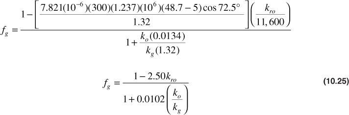
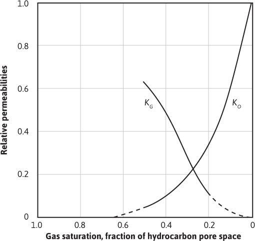
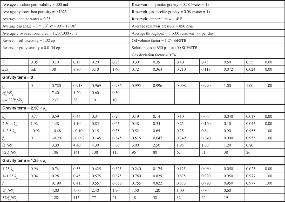
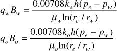
The use of Eq. (10.23) is illustrated using the data given by Welge for the Mile Six Pool, Peru, where advantage was taken of good gravitational segregation characteristics to improve recovery.10 Pressure maintenance by gas injection has been practiced since 1933 by returning produced gas and other gas to the gas cap so that reservoir pressure has been maintained within 200 psi of its initial value. Figure 10.12 shows the average relative permeability characteristics of the Mile Six Pool reservoir rock. As is common in gas-oil systems, the saturations are expressed in percentages of the hydrocarbon porosity, and the connate water, being immobile, is considered as part of the rock. The other pertinent reservoir rock and fluid data are given in Table 10.2. Substituting these data in Eq. (10.25),
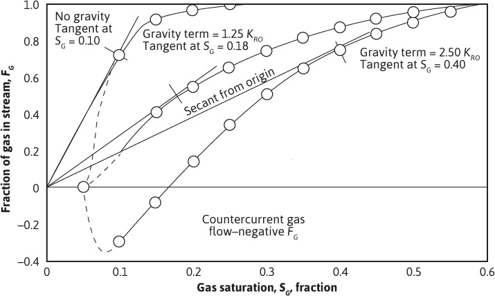
The values of fg have been calculated in Table 10.2 for three conditions: (1) assuming negligible gravitational segregation by using Eq. (10.24); (2) using the gravitational term equal to 2.50kro for the Mile Six Pool, Eq. (10.25); and (3) assuming the gravitational term equals 1.25kro, or half the value at Mile Six Pool. The values of fg for these three conditions are shown plotted in Fig. 10.13. The negative values of fg for the conditions that existed in the Mile Six Pool indicate countercurrent gas flow (i.e., gas updip and oil downdip) in the range of gas saturations between an assumed critical gas saturation of 5% and about 17%.
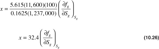
The distance of advance of any gas saturation plane may be calculated for the Mile Six Pool, using Eq. (10.15), replacing water as the displacing fluid by gas, or
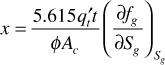
In 100 days, then,
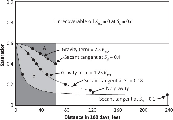
The values of the derivatives (∂fg/∂Sg) given in Table 10.2 have been determined graphically from Fig. 10.13. Figure 10.14 shows the plots of Eq. (10.26) to obtain the gas-oil distributions and the positions of the gas front after 100 days. The shape of the curves will not be altered for any other time. The distribution and fronts at 1000 days, for example, may be obtained by simply changing the scale on the distance axis by a factor of 10.
Welge showed that the position of the front may be obtained by drawing a secant from the origin as shown in Fig. 10.13.10 For example, the secant is tangent to the lower curve at 40% gas saturation. Then, in Fig. 10.14, the front may be found by dropping a perpendicular from the 40% gas saturation as indicated. This will balance the areas of the S-shaped curve, which was done by trial and error in Fig. 10.10 for water displacement. In the case of water displacement, the secant should be drawn, not from the origin, but from the connate water saturation, as indicated by the dashed line in Fig. 10.9. This is tangent at a water saturation of 60%. Referring to Fig. 10.10, the 240-day front is seen to occur at 60% water saturation. Owing to the presence of an initial transition zone, the fronts at 60 days and 120 days occur at slightly lower values of water saturation.
The much greater displacement efficiency with gravity segregation than without is apparent from Fig. 10.14. Since the permeability to oil is essentially zero at 60% gas saturation, the maximum recovery by gas displacement and gravity drainage is 60% of the initial oil in place. Actually, some small permeability to oil exists at even very low oil saturations, which explains why some fields may continue to produce at low rates for quite long periods after the pressure has been depleted. The displacement efficiency may be calculated from Fig. 10.14 by the measurement of areas. For example, the displacement efficiency at Mile Six Pool with full gravity segregation is in excess of

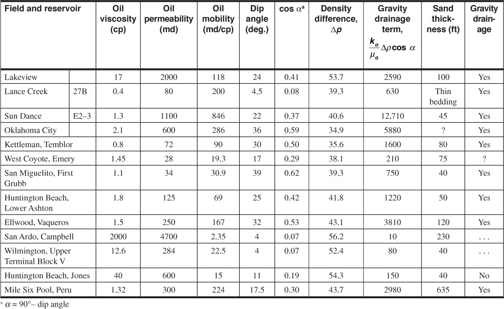
If the gravity segregation had been half as effective, the recovery would have been about 60%; without gravity segregation, the recovery would have been only 24%. These recoveries are expressed as percentages of the recoverable oil. In terms of the initial oil in place, the recoveries are only 60% as large, or 52.4%, 36.0%, and 14.4%, respectively. Welge, Shreve and Welch, Kern, and others have extended the concepts presented here to the prediction of gas-oil ratios, production rates, and cumulative recoveries, including the treatment of production from wells behind the displacement front.10,11,12 Smith has used the magnitude of the gravity term [(ko/μo)(ρo – ρg) cos α] as a criterion for determining those reservoirs in which gravity segregation is likely to be of considerable importance.13 The data of Table 10.3 indicate that this gravity term must have a value above about 600 in the units used to be effective. An inspection of Eq. (10.23), however, shows that the throughput velocity  is also of primary importance.
Table 10.3 Gravity Drainage Experience (after R. H. Smith, Except for Mile Six Pool13)
One interesting application of gravity segregation is to the recovery of updip or “attic” oil in active water-drive reservoirs possessing good gravity segregation characteristics. When the structurally highest well(s) has gone to water production, high-pressure gas is injected for a period. This gas migrates updip and displaces the oil downdip, where it may be produced from the same well in which the gas was injected. The injected gas is, of course, unrecoverable.
It appears from the previous discussions and examples that water is generally more efficient than gas in displacing oil from reservoir rocks, mainly because (1) the water viscosity is of the order of 50 times the gas viscosity and (2) the water occupies the less conductive portions of the pore spaces, whereas the gas occupies the more conductive portions. Thus, in water displacement, the oil is left to the central and more conductive portions of the pore channels, whereas in gas displacement, the gas invades and occupies the more conductive portions first, leaving the oil and water to the less conductive portions. What has been said of water displacement is true for preferentially water wet (hydrophilic) rock, which is the case for most reservoir rocks. When the rock is preferentially oil wet (hydrophobic), the displacing water will invade the more conductive portions first, just as gas does, resulting in lower displacement efficiencies. In this case, the efficiency by water still exceeds that by gas because of the viscosity advantage that water has over gas.
Oil is produced from volumetric, undersaturated reservoirs by expansion of the reservoir fluids. Down to the bubble-point pressure, the production is caused by liquid (oil and connate water) expansion and rock compressibility (see Chapter 6, section 6.6). Below the bubble point, the expansion of the connate water and the rock compressibility are negligible, and as the oil phase contracts owing to release of gas from solution, production is a result of expansion of the gas phase. When the gas saturation reaches the critical value, free gas begins to flow. At fairly low gas saturations, the gas mobility, kg/μg, becomes large, and the oil mobility, ko/μo, becomes small, resulting in high gas-oil ratios and in low oil recoveries, usually in the range of 5% to 25%.
Because the gas originates internally within the oil, the method described in the previous section for the displacement of oil by external gas drive is not applicable. In addition, constant pressure was assumed in the external displacement so that the gas and oil viscosities and volume factors remained constant during the displacement. With internal gas drive, the pressure drops as production proceeds, and the gas and oil viscosities and volume factors continually change, further complicating the mechanism.
Because of the complexity of the internal gas drive mechanism, a number of simplifying assumptions must be made to keep the mathematical forms reasonably simple. The following assumptions, generally made, do reduce the accuracy of the methods but, in most cases, not appreciably:
1. Uniformity of the reservoir at all times regarding porosity, fluid saturations, and relative permeabilities. Studies have shown that the gas and oil saturations about wells are surprisingly uniform at all stages of depletion.
2. Uniform pressure throughout the reservoir in both the gas and oil zones. This means the gas and oil volume factors, the gas and oil viscosities, and the solution gas will be the same throughout the reservoir.
3. Negligible gravity segregation forces
4. Equilibrium at all times between the gas and the oil phases
5. A gas liberation mechanism that is the same as that used to determine the fluid properties
6. No water encroachment and negligible water production
Several methods appear in the literature for predicting the performance of internal gas drive reservoirs from their rock and fluid properties. Three are discussed in this chapter: (1) Muskat’s method, (2) Schilthuis’s method, and (3) Tarner’s method.14,15,16 These methods relate the pressure decline to the oil recovery and the gas-oil ratio.
The reader will recall that the material balance is successful in predicting the performance of volumetric reservoirs down to pressures at which free gas begins to flow. In the study of the Kelly-Snyder Field, Canyon Reef Reservoir, for example, in Chapter 6, section 6.4, the produced gas-oil ratio was assumed to be equal to the dissolved gas-oil ratio, down to the pressure at which the gas saturation reached 10%, the critical gas saturation assumed for that reservoir. Below this pressure (i.e., at higher gas saturations), both gas and oil flow to the wellbores, their relative rates being controlled by their viscosities, which change with pressure, and by their relative permeabilities, which change with their saturations. It is not surprising, then, that the material balance principle (static) is combined with the producing gas-oil ratio equation (dynamic) to predict the performance at pressures at which the gas saturation exceeds the critical value.
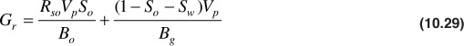
In the Muskat method, the values of the many variables that affect the production of gas and oil and the values of the rates of changes of these variables with pressure are evaluated at any stage of depletion (pressure). Assuming these values hold for a small drop in pressure, the incremental gas and oil production can be calculated for the small pressure drop. These variables are recalculated at the lower pressure, and the process is continued to any desired abandonment pressure. To derive the Muskat equation, let Vp be the reservoir pore volume in barrels. Then, the stock-tank barrels of oil remaining Nr at any pressure are given by
Differentiating with respect to pressure,
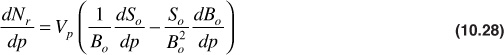
The gas remaining in the reservoir, both free and dissolved, at the same pressure, in standard cubic feet, is
Differentiating with respect to pressure,
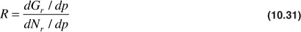
If reservoir pressure is dropping at the rate dp/dt, then the current or producing gas-oil ratio at this pressure is
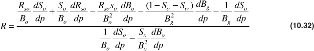
Substituting Eqs. (10.28) and (10.30) in Eq. (10.31),
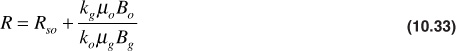
Equation (10.32) is simply an expression of the material balance for volumetric, undersaturated reservoirs in differential form. The producing gas-oil ratio may also be written as
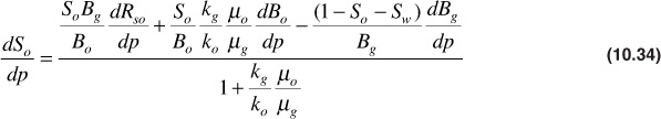
Equation (10.33) applies both to the flowing free gas and to the solution gas that flows to the wellbore in the oil. These two types of gas make up the total surface producing gas-oil ratio, R, in SCF/STB. Equation (10.33) may be equated to Eq. (10.32) and solved for dSo/dp to give
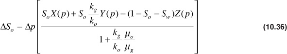
To simplify the handling of Eq. (10.34), the terms in the numerator that are functions of pressure may only be grouped together and given the group symbols X(p), Y(p), and Z(p) as follows:
Using these group symbols and placing Eq. (10.34) in an incremental form,
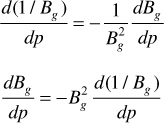
Equation (10.36) gives the change in oil saturation that accompanies a pressure drop, Δp. The functions X(p), Y(p), and Z(p) are obtained from the reservoir fluid properties using Eq. (10.35). The values of the derivatives dRso/dp, dBo/dp, and dBg/dp are found graphically from the plots of Rso, Bo, and Bg versus pressure. It has been found that when determining dBg/dp, the numbers are more accurately obtained by plotting 1/Bg versus pressure. When this is done, the following substitution is used:
In calculating ΔSo for any pressure drop Δp, the values of So, X(p), Y(p), Z(p), kg/ko, and μo/μg at the beginning of the interval may be used. Better results will be obtained, however, if values at the middle of the pressure drop interval are used. The value of So at the middle of the interval can be closely estimated from the ΔSo value for the previous interval and the value of kg/ko used corresponding to the estimated midinterval value of the oil saturation. In addition to Eq. (10.36), the total oil saturation must be calculated. This is done by simply multiplying the value of ΔSo/Δp by the pressure drop, Δp, and then subtracting the ΔSo from the oil saturation value that corresponds to the pressure at the beginning of the pressure drop interval, as shown in the following equation:
where j corresponds to the pressure at the end of the pressure increment and j – 1 corresponds to the pressure at the beginning of the pressure increment.
The following procedure is used to solve for the ΔSo for a given pressure drop Δp:
1. Plot Rso, Bo, and Bg or 1/Bg versus pressure and determine the slope of each plot.
2. Solve Eq. (10.36) for ΔSo/Δp using the oil saturation that corresponds to the initial pressure of the given Δp.
3. Estimate Soj using Eq. (10.38).
4. Solve Eq. (10.36) using the oil saturation from step 3.
5. Determine an average value for ΔSo/Δp from the two values calculated in steps 2 and 4.
6. Using (ΔSo/Δp)ave, solve for Soj using Eq. (10.38). This value of Soj becomes So(j–1) for the next pressure drop interval.
7. Repeat steps 2 through 6 for all pressure drops of interest.
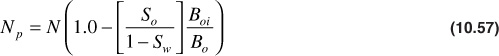
The Schilthuis method begins with the general material balance equation, which reduces to the following for a volumetric, undersaturated reservoir, using the single-phase formation volume factor:
Notice that this equation contains variables that are a function of only the reservoir pressure, Bt, Bg, Rsoi, and Bti, and the unknown variables, Rp and Np. Rp, of course, is the ratio of cumulative oil production, Np, to cumulative gas production, Gp. To use this equation as a predictive tool for Np, a method must be developed to estimate Rp. The Schilthuis method uses the total surface producing gas-oil ratio or the instantaneous gas-oil ratio, R, defined previously in Eq. (10.33) as
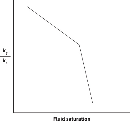
The first term on the right-hand side of Eq. (10.33) accounts for the production of solution gas, and the second term accounts for the production of free gas in the reservoir. The second term is a ratio of the gas to oil flow equations discussed in Chapter 8. To calculate R with Eq. (10.33), information about the permeabilities to gas and oil is required. This information is usually known from laboratory measurements as a function of fluid saturations and is often available in graphic form (see Fig. 10.15). The fluid saturation equation is also needed:
where
SL is the total liquid saturation (i.e., SL = Sw + So, which also equals 1 – Sg).
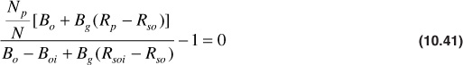
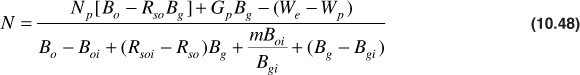
The solution of this set of equations to obtain production values requires a trial-and-error procedure. First, the material balance equation is rearranged to yield the following:
All the parameters in Eq. (10.41) are known as functions of pressure from laboratory studies except Np/N and Rp. When the correct values of these two variables are used in Eq. (10.41) at a given pressure, then the left-hand side of the equation equals zero. The trial-and-error procedure follows this sequence of steps:
1. Guess a value for an incremental oil production (ΔNp/N) that occurs during a small drop in the average reservoir pressure (Δp).
2. Determine the cumulative oil production to pressure pj = pj–1 – Δp by adding all the previous incremental oil productions to the guess during the current pressure drop. The subscript, j – 1, refers to the conditions at the beginning of the pressure drop and j to the conditions at the end of the pressure drop.
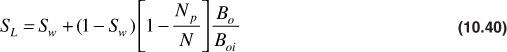
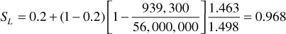
3. Solve the total liquid saturation equation, Eq. (10.40), for SL at the current pressure of interest.
4. Knowing SL, determine a value for kg/ko from permeability ratio versus saturation information, and then solve Eq. (10.33) for Rj at the current pressure.
5. Calculate the incremental gas production using an average value of the gas-oil ratio over the current pressure drop:
6. Determine the cumulative gas production by adding all previous incremental gas productions in a similar manner to step 2, in which the cumulative oil was determined.
7. Calculate a value for Rp with the cumulative oil and gas amounts.
8. With the cumulative oil recovery from step 2 and the Rp from step 7, solve Eq. (10.41) to determine if the left-hand side equals zero. If the left-hand side does not equal zero, then a new incremental recovery should be guessed and the procedure repeated until Eq. (10.41) is satisfied.
Any one of a number of iteration techniques can be used to assist in the trial-and-error procedure. One that has been used is the secant method,17 which has the following iteration formula:
To apply the secant method to the foregoing procedure, the left-hand side of Eq. (10.41) becomes the function, f, and the cumulative oil recovery becomes x. The secant method provides the new guess for oil recovery, and the sequence of steps is repeated until the function, f, is zero or within a specified tolerance (e.g., ±10–4). The solution procedure described earlier is fairly easy to program on a computer. The authors are keenly aware that programs like Excel can be used to solve this problem without writing a separate program to include a solution procedure like the secant method. However, an understanding of the secant method may help the reader to visualize how these solvers work, and for that reason, it is presented here.
The Tarner method for predicting reservoir performance by internal gas drive is presented in a form proposed by Tracy.18 Neglecting the formation and water compressibility terms, the general material balance in terms of the single-phase oil formation volume factor may be written as follows:
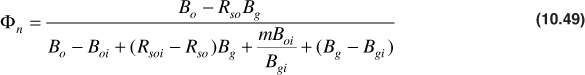
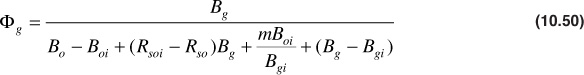
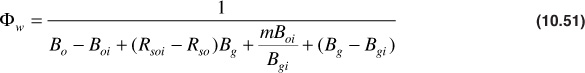
Tracy suggested writing
where Фn, Фg, and Фw are simply a convenient collection of many terms, all of which are functions of pressure, except the ratio m, the initial free gas-to-oil volume. The general material balance equation may now be written as
Applying this equation to the case of a volumetric, undersaturated reservoir,
In progressing from the conditions at any pressure, pj–1, to a lower pressure, pj, Tracy suggested the estimation of the producing gas-oil ratio, R, at the lower pressure rather than estimating the production ΔNp during the interval, as we did in the Schilthuis method. The value of R may be estimated by extrapolating the plot of R versus pressure, as calculated at the higher pressure. Then the estimated average gas-oil ratio between the two pressures is given by Eq. (10.43):
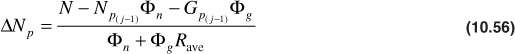
From this estimated average gas-oil ratio for the Δp interval, the estimated production, ΔNp, for the interval is made using Eq. (10.53) in the following form:
From the value of ΔNp in Eq. (10.56), the value of Npj is found:
In addition to these equations, the total liquid saturation equation is required, Eq. (10.40). The solution procedure becomes as follows:
1. Calculate the values of Фn and Фg as a function of pressure.
2. Estimate a value for Rj in order to calculate an Rave for a pressure drop of interest, Δp.
3. Calculate ΔNp by rearranging Eq. (10.54) to give
4. Calculate the total oil recovery from Eq. (10.55).
5. Determine kg/ko by calculating the total liquid saturation, SL, from Eq. (10.40) and using kg/ko versus saturation information.
6. Calculate a value of Rj by using Eq. (10.33), and compare it with the assumed value in step 2. If these two values agree within some tolerance, then the ΔNp calculated in step 3 is correct for this pressure drop interval. If the value of Rj does not agree with the assumed value in step 2, then the calculated value should be used as the new guess and steps 2 through 6 repeated.
As a further check, the value of Rave can be recalculated and Eq. (10.56) solved for ΔNp. Again, if the new value agrees with what was previously calculated in step 3 within some tolerance, it can be assumed that the oil recovery is correct. The three methods are illustrated in Example 10.1.
Example 10.1 Calculating Oil Recovery as a Function of Pressure
This example uses the (1) Muskat, (2) Schilthuis, and (3) Tarner methods for an undersaturated, volumetric reservoir. The recovery is calculated for the first 200-psi pressure increment from the initial pressure down to a pressure of 2300 psia.
Given
Initial reservoir pressure = 2500 psia
Initial reservoir temperature = 180°F
Initial oil in place = 56 × 106 STB
Initial water saturation = 0.20
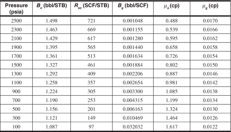
Fluid property data are given in Table 10.4.
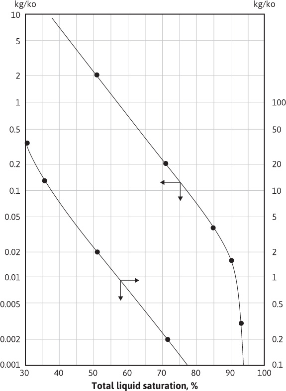
Permeability ratio data are plotted in Fig. 10.16.
Table 10.4 Fluid Property Data for Example 10.1
Figure 10.16 Permeability ratio relationship for Example 10.1.
Solution
The Muskat method involves the following sequence of steps:
1. Rso, Bo, and 1/Bg are plotted versus pressure to determine the slopes. Although the plots are not shown, the following values can be determined:

The values of X(p), Y(p), and Z(p) are tabulated as follows, as a function of pressure:
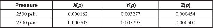
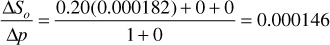
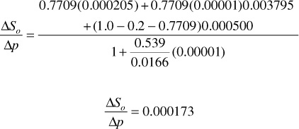
2. Calculate ΔSo/Δp using X(p), Y(p), and Z(p) at 2500 psia:
Soj = 0.80 – 200(0.000146) = 0.7709
4. Calculate ΔSo/Δp using the Soj from step 3 and X(p), Y(p), and Z(p) at 2300 psia:
5. Calculate the average ΔSo/Δp:
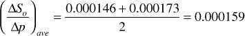
6. Calculate Soj using (ΔSoΔp)ave from step 5:
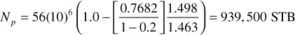
Soj = 0.8 – 0.000159(200) = 0.7682
This value of So can now be used to calculate the oil recovery that has occurred down to a pressure of 2300 psia:
Because the Schilthuis method involves an interactive procedure, an iterative solver, like Excel’s solver, is used to assist in the solution. For this problem, Np/N is the guess value that the solver will use to solve Eq. (10.41). The solver requires one guess value of Np/N to begin the iteration process.
1. Assume incremental oil recovery:

2. Calculate SL:
3. Determine kg/ko from Fig. 10.16 and calculate R:
4. Calculate incremental gas recovery:
5. Calculate Rp:
6. Use Excel’s solver function to solve Eq. (10.41) iteratively by changing Np/N until the left-hand side of Eq. (10.41) is equal to zero:
Using this method, the correct value of fractional oil recovery down to 2300 psia is 0.0165. To compare with the Muskat method, the recovery ratio must be multiplied by the initial oil in place, 56 M STB, to yield the total cumulative recovery:
Np = 56(10)6 (0.0167) = 935,200 STB
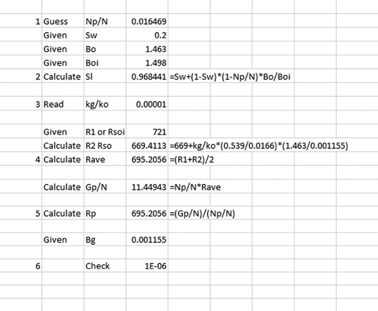
The Tarner method requires the following steps:
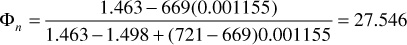
1. Calculate Фn and Фg at 2300 psia:
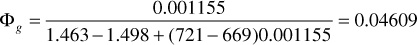
2. Assume Rj = 670 SCF/STB, which is just slightly larger than Rso, suggesting that only a very small amount of gas is flowing to the wellbore and is being produced:
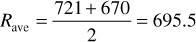
3. Calculate ΔNp:
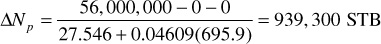
4. Calculate Np:
Np = ΔNp = 939,300 STB
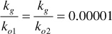
5. Determine kg/ko:
From this value of SL, the permeability ratio, kg/ko, can be obtained from Fig. 10.16. Since the curve is off the plot, a very small value of kg/ko = 0.00001 is estimated.
6. Calculate Rj and compare it with the assumed value in step 2:
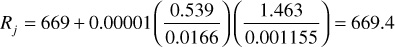
This value agrees very well with the value of 670 that was assumed in step 2, satisfying the constraints of the Tarner method. For the data given in this example, the three methods of calculation yielded values of Np that are within 0.5%. This suggests that any one of the three methods may be used to predict oil and gas recovery, especially considering that many of the parameters used in the equations could be in error more than 0.5%.
The intent of this chapter was to present fundamental concepts that can help reservoir engineers understand the immiscible displacement of oil and gas. Many practicing engineers will need to add the tool of reservoir simulation to the concepts discussed in this chapter. The simulation of reservoirs involves many of the equations that have been presented in this chapter, along with much more involved mathematics and computer programming. The interested reader is referred to a number of published works that describe the important field of reservoir simulation.19–22
10.1 (a) A rock 10 cm long and 2 cm2 in cross section flows 0.0080 cm3/sec of a 2.5-cp oil under a 1.5-atm pressure drop. If the oil saturates the rock 100%, what is its absolute permeability?
(b) What will be the rate of 0.75-cp brine in the same core under a 2.5-atm pressure drop if the brine saturates the rock 100%?
(c) Is the rock more permeable to the oil at 100% oil saturation or to the brine at 100% brine saturation?
(d) The same core is maintained at 40% water saturation and 60% oil saturation. Under a 2.0-atm pressure drop, the oil flow is 0.0030 cm3/sec and the water flow is 0.004 cm3/sec. What are the effective permeabilities to water and to oil at these saturations?
(e) Explain why the sum of the two effective permeabilities is less than the absolute permeability.
(f) What are the relative permeabilities to oil and water at 40% water saturation?
(g) What is the relative permeability ratio ko/kw at 40% water saturation?
(h) Show that the effective permeability ratio is equal to the relative permeability ratio.
10.2 The following permeability data were measured on a sandstone as a function of its water saturation:
(a) Plot the relative permeabilities to oil and water versus water saturation on Cartesian coordinate paper.
(b) Plot the relative permeability ratio versus water saturation on semilog paper.
(c) Find the constants a and b in Eq. (10.3) from the slope and intercept of your graph. Also find a and b by substituting two sets of data in Eq. (10.3) and solving simultaneous equations.
(d) If μo = 3.4 cp, μw = 0.68 cp, Bo = 1.50 bbl/STB, and Bw = 1.05 bbl/STB, what is the surface watercut of a well completed in the transition zone where the water saturation is 50%?
(e) What is the reservoir watercut in part (d)?
(f) What percentage of recovery will be realized from this sandstone under high-pressure water drive from that portion of the reservoir above the transition zone invaded by water? The initial water saturation above the transition zone is 30%.
(g) If water drive occurs at a pressure below saturation pressure such that the average gas saturation is 15% in the invaded portion, what percentage of recovery will be realized? The average oil volume factor at the lower pressure is 1.35 bbl/STB and the initial oil volume factor is 1.50 bbl/STB.
(h) What fraction of the absolute permeability of this sandstone is due to the least permeable pore channels that make up 20% of the pore volume? What fraction is due to the most permeable pore channels that make up 25% of the pore volume?
10.3 Given the following reservoir data,
Throughput rate = 1000 bbl/day
Average porosity = 18%
Initial water saturation = 20%
Cross-sectional area = 50,000 ft2
Water viscosity = 0.62 cp
ko/kw versus Sw data in Figs. 10.1 and 10.2
assume zero transition zone and
(a) Calculate fw and plot versus Sw.
(b) Graphically determine ∂fw/∂Sw at a number of points and plot versus Sw.
(c) Calculate ∂fw/∂Sw at several values of Sw using Eq. (10.17), and compare with the graphical values of part (b).
(d) Calculate the distances of advance of the constant saturation fronts at 100, 200, and 400 days. Plot on Cartesian coordinate paper versus Sw. Equalize the areas within and without the flood front lines to locate the position of the flood fronts.
(e) Draw a secant line from Sw = 0.20 tangent to the fw versus Sw curve in part (b), and show that the value of Sw at the point of tangency is also the point at which the flood front lines are drawn.
(f) Calculate the fractional recovery when the flood front first intercepts a well, using the areas of the graph of part (d). Express the recovery in terms of both the initial oil in place and the recoverable oil in place (i.e., recoverable after infinite throughput).
(g) To what surface watercut will a well rather suddenly rise when it is just enveloped by the flood fronts? Use Bo = 1.50 bbl/STB and Bw = 1.05 bbl/STB.
(h) Do the answers to parts (f) and (g) depend on how far the front has traveled? Explain.
10.4 Show that for radial displacement where rw <<,
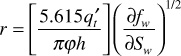
where r is the distance a constant saturation front has traveled.
10.5 Given the following reservoir data,
Absolute permeability = 400 md
Hydrocarbon porosity = 15%
Connate water = 28%
Dip angle = 20°
Cross-sectional area = 750,000 ft2
Oil viscosity = 1.42 cp
Gas viscosity = 0.015 cp
Reservoir oil specific gravity = 0.75
Reservoir gas specific gravity = 0.15 (water = 1)
Reservoir throughput at constant pressure = 10,000 bbl/day
(a) Calculate and plot the fraction of gas, fg, versus gas saturation similar to Fig. 10.13 both with and without the gravity segregation term.
(b) Plot the gas saturation versus distance after 100 days of gas injection both with and without the gravity segregation term.
(c) Using the areas of part (b), calculate the recoveries behind the flood front with and without gravity segregation in terms of both initial oil and recoverable oil.
10.6 Derive an equation, including a gravity term similar to Eq. (10.23) for water displacing oil.
10.7 Rework the water displacement calculation of Table 10.1, and include a gravity segregation term. Assume an absolute permeability of 500 md, a dip angle of 45°, and a density difference of 20% between the reservoir oil and water and an oil viscosity of 1.6 cp. Plot water saturation versus distance after 240 days and compare with Fig. 10.11.

10.8 Continue the calculations of Problem 10.1 down to a reservoir pressure of 100 psia, using
(a) Muskat method
(b) Schilthuis method
(c) Tarner method
1. G. P Willhite, Waterflooding, Vol. 3, Society of Petroleum Engineers, 1986.
2. F. F. Craig, The Reservoir Engineering Aspects of Waterflooding, Society of Petroleum Engineers, 1993.
3. L. W. Lake, Enhanced Oil Recovery, Prentice Hall, 1989.
4. D. W. Green and G. P. Willhite, Enhanced Oil Recovery, Vol. 6, Society of Petroleum Engineers, 1998.
5. E. D. Holstein, ed., Petroleum Engineering Handbook, Vol. 5, Reservoir Engineering and Petrophysics, Society of Petroleum Engineers, 2007.
6. R. D. Wycoff, H. G. Botset, and M. Muskat, “Mechanics of Porous Flow Applied to Water-Flooding Problems,” Trans. AlME (1933), 103, 219.
7. R. L. Slobod and B. H. Candle, “X-ray Shadowgraph Studies of Areal Sweep Efficiencies,” Trans. AlME (1952), 195, 265.
8. S. E. Buckley and M. C. Leverett, “Mechanism of Fluid Displacement in Sands,” Trans. AlME (1942), 146, 107.
9. J. G. Richardson and R. J. Blackwell, “Use of Simple Mathematical Models for Predicting Reservoir Behavior,” Jour. of Petroleum Technology (Sept. 1971), 1145.
10. H. J. Welge, “A Simplified Method for Computing Oil Recoveries by Gas or Water Drive,” Trans. AlME (1952), 195, 91.
11. D. R. Shreve and L. W. Welch Jr., “Gas Drive and Gravity Drainage Analysis for Pressure Maintenance Operations,” Trans. AlME (1956), 207, 136.
12. L. R. Kern, “Displacement Mechanism in Multi-well Systems,” Trans. AlME (1952), 195, 39.
13. R. H. Smith reported by J. A. Klotz, “The Gravity Drainage Mechanism,” Jour. of Petroleum Technology (Apr. 1953), 5, 19.
14. M. Muskat, “The Production Histories of Oil Producing Gas-Drive Reservoirs,” Jour. of Applied Physics (1945), 16, 147.
15. E. T. Guerrero, Practical Reservoir Engineering, Petroleum Publishing Co., 1968.
16. J. Tarner, “How Different Size Gas Caps and Pressure Maintenance Programs Affect Amount of Recoverable Oil,” Oil Weekly (June 12, 1944), 144, 32–34.
17. J. B. Riggs, An Introduction to Numerical Methods for Chemical Engineers, Texas Tech. University Press, 1988.
18. G. W. Tracy, “Simplified Form of the Material Balance Equation,” Trans. AlME (1955), 204, 243.
19. T. Ertekin, J. H. Abou-Kassem, and G. R. King, Basic Applied Reservoir Simulation, Vol. 10, Society of Petroleum Engineers, 2001.
20. J. Fanchi, Principles of Applied Reservoir Simulation, 3rd ed., Elsevier, 2006.
21. C. C. Mattax and R. L. Dalton, Reservoir Simulation, Vol. 13, Society of Petroleum Engineers, 1990.
22. M. Carlson, Practical Reservoir Simulation, PennWell Publishing, 2006.