In the previous chapters, we have examined the progression of voter preferences over the timeline of presidential elections. We have focused primarily on national trial-heat polls from April to November, for the last fifteen elections. In this chapter, we summarize what we have learned in general and consider what it tells us about the predictability of the different presidential elections we have examined.
Our results at times seem to offer contradictions. Aggregate vote intentions seem to be stable over the campaign. Yet they obviously change, if mostly glacially, from April to November. Early polls from April appear to incorporate a considerable amount of extraneous information that does not survive to impact the election. Yet early polls do contain information that matters in November. Voters in early polls do not seem to take the economy into account very much. But by November, the economy shapes the result. In short, if we consider whether the campaign events from April to November are crucial or irrelevant to shaping the election, the answer is somewhere in between the two extremes.
Throughout this book we have structured the discussion in terms of modeling the campaign as a time series. We ask whether specific campaigns have their unique equilibria. The answer is a decisive yes. Yet, importantly, these equilibria often move, if slowly, over the campaign. Results from any one poll will have noise from sampling error, so we can never track the vote with total precision. Yet even if we could view it, the precise record of vote intentions would include short-term wobbles around the equilibrium of the moment. Every poll should be viewed within the context of past readings for the best guess regarding how much observed change is due to sampling error and what is real. And the real part can be a short-term blip or a change in the long-run equilibrium. Even if most true change is of the short-term variety, it is the small but real change that in the long-run is of electoral importance. Events may produce short-term bounces. But they may also leave a residue in the form of small long-term bumps. Except for the period immediately before the election, only the bumps last to Election Day.
We have also discovered some facts about the pace of change over the campaign timeline. As a very general rule, both long-term and short-term sources of change decrease as the campaign progresses. During the final 60 days of the campaign—when candidates have been chosen and the formal campaigning begun—very little change occurs. Yet even modest short-term shifts matter if they occur close to Election Day.
Three periods stand out as the most important of the campaign time-line, as having the greatest impact on voter choice—the beginning of the election year, the convention season, and the final days of the campaign. Consider first the very outset of the election year, 200 to 300 days before Election Day. With the nomination process under way, this period is often the voters’ initial introduction to the eventual candidates. As voters gain what are often their first impressions of the candidates, preferences begin to take shape and eventually harden.
At convention time, the national vote division in the polls often gets considerably upended, as if the electorate is reshuffling. As the conventions take place, voters are especially attentive. In the days dominated by broadcast networks and print media, citizens can hardly avoid news of the conventions, and the shows the parties put on. It is easy to imagine that many voters shift as a result of the conventions, and the evidence indicates that they do. (This evidently is true even in recent elections with a growing cable and satellite television viewership and a declining print media.) The vote margin coming out of the conventions is different than that going in. And if we measure the consequences a few weeks after the dust of the final convention settles, the result is a decisive bump in the polls for whoever had the best convention—not a fading bounce.
The final days of the campaign present another period that concentrates political minds. Most voters have made up their minds long before the last minutes. But the small minority that has not yet decided can upset the best electoral predictions. Moreover, as we have seen, the gap between the final polls and the actual vote is also determined by composition effects—that is, likely voters and actual voters are not necessarily the same. Likely voters who do not vote are influenced by the events of the campaign in terms of the vote intentions they offer in surveys. Meanwhile, last-minute deciders who had not impacted pre-election surveys tend to split close to 50–50, helping to make elections appear closer.
When we speak of the equilibrium value of vote intentions, we are, in effect, speaking of the fundamentals of the campaign as they evolve. And what are these fundamentals that generate the long-lasting evolution of voter preferences over the campaign? In short, what drives the moving equilibrium?
The economy is an important factor. As the campaign progresses, perceptions of the degree of economic growth tend to push the arrow of change toward or against the incumbent presidential party. Measured by the objective economy or by subjective evaluations by the electorate, the economy helps to drive the moving equilibrium.
The equilibrium is a function of other factors as well. Some are captured by simply measuring the sitting president’s approval level, which is a good summary indicator of presidential performance. In terms of tangible influences, the relative closeness of the two candidates on ideology or policy issues matters. We measure ideological closeness by separately measuring public opinion and the candidates’ positions. From public opinion polls on issues (estimated via Stimson’s mood), we know that the more liberal the electorate, the more it votes Democratic. But variability in the parties’ ideological stances matter too. As either party platform moderates relative to its ideological base (as measured by Budge et al.’s scoring), it gains votes. This is exactly what theories (e.g., Downs 1957) predict will happen with a rational, issue-oriented electorate. Besides proximity, party identification plays a role—for a presidential candidate, it is good to be associated with a popular party.
The different fundamentals come into focus at different times. The economy begins to influence electoral preferences early in the election year, though its impact continues to grow over the campaign. Political factors matter later, around the time of the conventions. At the beginning of the fall general election campaign, vote intentions reveal the ultimate Election Day outcome. Preferences change only slightly thereafter, and mostly due to the growing impact of voters’ internal fundamentals. To a large extent, then, the effects of campaigns are fairly predictable. Over the campaign timeline, voters take stock of economic conditions and the political choice before them and form “enlightened” electoral preferences (Gelman and King 1993). How this happens—whether the result of priming or learning, whether activated by the behavior of the candidates’ campaigns or the “need to decide” as the election draws nearer—is unclear. What is clear is that certain knowable things matter on Election Day, and they actually are at least partly knowable in advance, even toward the beginning of the election year. They are not perfectly known at that point in time, however, as the fundamentals do change over the course of the election year.
We know we cannot measure all the fundamentals of presidential campaigns from observable variables. Some elections seem heavily influenced by important one-time events. Others may be influenced by forces that are simply intangible. To understand Republican Nixon’s victory over Democrat Humphrey in 1968, it is necessary to move beyond statistical analysis to take into account President Johnson’s unpopular Vietnam War. To account for Democrat Jimmy Carter’s victory over Republican Gerald Ford in 1976, one must refer to the recent history of the Watergate scandal.
A possible example of intangibles at work is the 2000 election. By all statistical forecasts, Democrat Al Gore should have defeated Republican George W. Bush. Although Gore actually won the popular vote by a narrow margin, the truth is that Bush did considerably better than suggested by all predictive models based on the economy and presidential performance. Was this due to the aftermath of President Clinton’s affair with Monica Lewinsky? Was it just a bad job of campaigning by Gore (or a great campaign by Bush)? Some (e.g., Vavreck 2009) cite Gore’s failure to take proper credit for a good economy (and also Bush’s successful “insurgent” campaign). Others (e.g., Fiorina, Abrams, and Pope 2003) say Gore’s problem was a leftward shift instead of adopting a more centrist position. Or maybe Bush won because the economy really was not as prosperous as it was thought to be (Bartels and Zaller 2001). We still cannot say for sure.
Back in chapter 2, we displayed poll results for our fifteen election campaigns, day by day, from April to November. In this section, we again present poll results over the fifteen campaigns, but this time with an eye for what the polls at any moment signify for the final outcome. In other words, we present the daily readings of the probable Democratic versus Republican win, conditional on the latest trial-heat polls. In effect, as if we could go back in time, we depict what informed observers of the contemporary polls might have or should have predicted about the November election. We ask: What would observers back in time have expected about the outcome if they had the statistical knowledge about how polls relate to the final vote that we present in this book? We also take a further step. We ask: How would these knowledgeable observers change their expectations if they knew further information about the likely outcome from the knowable fundamentals, apart from trial-heat polls? Here we present day-to-day election predictions based on the combination of polls, economic growth, and presidential approval.1
This exercise is motivated by several objectives. One is to visualize in a few glances how predictable (or not) elections are when seen from advance information. Another is to visualize the gap between the strictly poll-based prediction and the secondary prediction that includes the fundamentals. A third motivation is to show the relevance of campaigns. At any one point in the campaign timeline, we gain a probabilistic prediction of the winner. The difference between the probability distribution on a given date (e.g., 60–40 that the Republican would win) and the final outcome (either a Republican or Democratic win) is one measure of the effect of the campaign yet to be conducted. There is a final, fourth motivation. Our analysis can reveal that some elections are harder to predict from a set of defined, tangible variables than others. As we will see, the prediction game involves a large set of prediction successes, plus a smaller set of prediction failures. The daily forecasts are shown in figures 8.1–8.3, ahead. The details of their construction follow directly.
For 200 days across 15 campaigns (3,000 observations), we observe the pooled polls reported over the previous seven days. (To identify polls observable on each date, we code the date as two days later than the midpoint of the polling period.) In many instances, of course, there are no polls over this seven-day window. In these instances, we report the vote intentions from the most recent poll, whenever that occurred. For every date (measured as the number of days before the election), we regress the final Democratic versus Republican vote on the seven-day poll results. The predictions from these 200 equations provide the vote projections. Then we use the degree of fit to estimate the probable outcome based on polls observed for that date.
As in chapter 5, the generic vote projection equation is
where VOTEj = the actual Democratic percentage of the two-party vote in year j, and VjT = the corresponding trial-heat poll division in year j on day T of the campaign. As per our usual procedure, and for interpretive convenience, the vote division is measured as deviations from a tied 50–50 vote.
If α were zero and β were unity, the projection  would be identical to the raw two-party vote division of the polls. But, as we have seen, early leads fade. The daily β estimates are thus all below 1.0. The vote projection equations can be used not only to obtain an expectation of the vote but also the variance around that expectation. The estimated variance in the error term, or
  , is used to estimate the probable outcome. Knowing , we estimate the cumulative normal density ΦYT at zero (50–50 split), that is, the probability of a Democratic victory in year Y based on the polls at time T.2 For the actual daily probabilities, we show the estimate at the time of the most recent poll. This way, every time there is a new poll reported, the probability can shift. For dates without a poll, the probability does not move since the informed voter at the time would possess no new polling information.
Construction of the fundamentals-based forecasts is different. Here, since the fundamentals affect the incumbent presidential party, we model the presidential party vote rather than the Democratic vote. Then we convert the incumbent party vote to a prediction for the Democratic candidate.3 Independent variables for the daily equations include the trial-heat polls (with the two-day lag as above), presidential approval, and the measure of Economic Growth, that is, per capita income growth, from chapter 6. Since the latter two measures are interpolated, they are admittedly imprecise for daily readings, though we do not attempt to lag them. In effect, we assume a forecast based on what an observer at the time might have “felt” about the political and economic environment rather than what he or she might have read or heard in terms of news reports about measures of the president’s popularity or the economy. Thus, while the movement of the trial heat–based prediction is discrete, changing only with a new poll or polls, the movement of the fundamentals prediction is continuous, shifting with each daily imputation of the model’s inputs.
The choice of variables for the fundamentals is parsimonious. There is no measure of macropartisanship, mood, or party platform ideology. As shown in chapter 6, these variables tend to be incorporated into the president’s approval rating. The president’s approval level is a proxy for these omitted variables, plus other factors in the political environment that matter but cannot be directly observed. Even so, it is not a perfect proxy, and so this analysis provides a conservative estimate of what we might have predicted based on the knowable fundamentals.
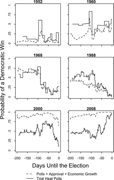
We follow the running forecasts of the vote over the campaign timelines of the fifteen elections. These elections are presented in three separate figures for three types of elections, each representing a unique political environment. Figure 8.1 shows a set of six contests without the sitting president on the ballot, a circumstance that usually results in a close election. Figure 8.2 follows the outcome over the campaign timeline for four elections in which the incumbent ran for reelection, but under some degree of political distress. Figure 8.3 shows the remaining set of five elections, in which the sitting president won reelection handily.
Figure 8.1 shows the data for the six contests in which the sitting president did not run. Only in 1952 did the outcome seem certain throughout the campaign. In that year the electorate was ready to elect Republican Dwight Eisenhower after twenty years of Democratic presidents. In the other five cases, on the basis of the polls alone, the outcome was volatile, with each candidate favored at some point in the timeline. The predictions incorporating the fundamentals showed more stability and certainty.
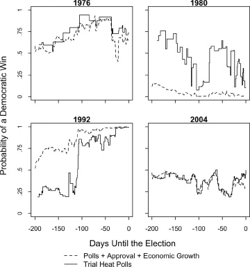
Figure 8.2 shows the data for the four campaigns in which the sitting president sought reelection in an uncertain environment. Three instances were presidential losses (Ford in 1976; Carter in 1980; Bush I in 1992). Of the four, only in 2004 did the president succeed (Bush II over Kerry).
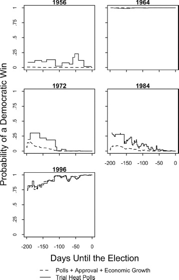
Figure 8.3 presents the final five examples. These are less interesting as they represent sitting presidents who basically coasted to reelection. In these five contests, the signs pointed to reelection throughout. The result should not have surprised.
Of the fifteen elections, nine showed variability in the likely outcome over the campaign. (The election of 1976 arguably is a close call.) Thus about half the time, the contest has meaning through much of the campaign and should not be treated as a foregone conclusion. First we look at the five instances of closely contested elections without the president running for reelection.
The 1960 contest (Kennedy versus Nixon) was close throughout. Kennedy led in the polls more often than not, and the poll-based predictions generally show him in a slight lead. Eight years later the 1968 contest showed Democrat Humphrey slightly favored in matchups with Nixon until the dissension-filled Democratic convention. Nixon’s lead in the fall looked safe, with a slight upturn of doubt toward the end.
Figure 8.1. Probable outcomes over the campaign time-line in six elections in which the incumbent president did not seek reelection. Trial-heat poll probabilities are from regression equations predicting the vote from the polls over the recent seven days. The “polls + approval + economic growth” predictions are from equations adding interpolated presidential approval and income growth. See the text for further details.
The 1988 contest was one in which the polls and the fundamentals started off at odds. On the basis of the trial-heat polls alone, it looked as though Democrat Dukakis was likely to defeat George H. W. Bush. By the end of the convention season, however, the polls turned toward Bush. Voters gravitated toward the fundamentals, which had Bush the winner all along.
The 2000 contest was one in which the polls and the fundamentals were at odds for much of the campaign. Republican Bush led Democrat Gore in the polls for most of the campaign, even though the fundamentals seemed to favor Gore. As discussed earlier, the 2000 election is a case in which the observable fundamentals suggested a stronger showing for Gore. In fact, Gore did surge at the end and, in fact, win the popular vote, while losing the contested Electoral College outcome.
The most recent nonincumbent race, of course, is 2008. Figure 8.1 shows that, on the basis of the polls alone, Obama was only the slight favorite for much of the year and became the underdog briefly after the conventions. But he became the likely choice after the Republican convention, and once the economy went into freefall in September. Importantly, the signal of the fundamentals was that this was an election for the Democrats to win all along.
Figure 8.2. Probable outcomes over the campaign timeline in four elections in which the incumbent president faced a strong reelection challenge. Trial-heat poll probabilities are from regression equations predicting the vote from the polls over the recent seven days. The “polls + approval + economic growth” predictions are from equations adding interpolated presidential approval and income growth. See the text for further details.
Figure 8.3 Probable outcomes over the campaign timeline in five elections in which the incumbent president coasted to reelection. Trial-heat poll probabilities are from regression equations predicting the vote from the polls over the recent seven days. The “polls + approval + economic growth” predictions are from equations adding interpolated presidential approval and income growth. See the text for further details.
Of the five close contests with a sitting president, the least close was 1976, where President Gerald Ford was a continual underdog, with a continuously low probability of reelection according to the polls. As measured, the fundamentals were not that unfavorable. Here is an instance in which the trial-heat poll predictions were more accurate than the fundamentals’ predictions (although Ford’s chances improved slightly toward the end). One big issue lurking in 1976 was Nixon’s Watergate scandal and Ford’s pardon of Nixon. Perhaps Jimmy Carter, the Democrat, was elected with the help of the unmeasured fundamental effect of the Watergate scandal.
In 1980, Carter’s reelection prospects against Reagan moved up and down with the polls, as shown in figure 8.2. The fundamentals this time worked very much against Carter, due to the poor economy and his unpopularity. This is a case in which the polls gravitated toward the fundamentals.
In 1992, it was G. H. W. Bush’s turn to be defeated by poor fundamentals. The early polls suggested he would probably defeat the unknown Bill Clinton in a matchup. But this changed following the conventions as the poll prediction turned in the direction of the fundamentals, which had Bush losing all along.
The 2004 election is our final example, and in this instance the embattled president escaped unscathed. Noteworthy about 2004 is that although the polls were close, they tended to place President Bush as the favorite, if not by as much as the fundamentals until late in the campaign. Staying close was not enough for Kerry to have much chance, as vote intentions usually move too slowly for that to happen.4
One lesson from figures 8.1–8.3 is that, since the probability of a Democratic versus a Republican president often undergoes meaningful changes over a campaign, the campaigns must matter. For any point on the time-line, the gap between the probability of a Democratic win and the actuality (0 or 100 percent) stands out as the effect of the remaining campaign period. In general, although the likely verdict can change, it changes less than commonly believed.
One way we know this is because the poll-based prediction tends to be more certain than the beliefs of investors who gamble on election outcomes. Presumably, the most informed and unbiased views are those of the gamblers who bet on elections to make money.5 Most election markets, both today and in the past, are winner-take-all markets, in which investors wager on the winner, given the candidates’ odds of victory.6 The important thing is that the price of a candidate registers the probability that he will win. We thus can directly compare these prices and the probabilities associated with our poll-based predictions as well as those including the fundamentals.
Interestingly, in recent elections, for which we have data from electronic election stock markets, prices have persistently overvalued underdog candidates (see Erikson and Wlezien 2008a).7 This is as if wagerers believe that electoral preferences are more volatile than they are in reality and overestimate the likelihood that the candidate who is behind can pull it out between the moment of the wager and Election Day. Assuming that market prices reflect informed opinion, the underdog bias carries an important implication: The campaign dynamics we have described in this book are less fluid than informed observers believe.
We can consider examples of election markets from recent elections, starting with IEM’s pioneering winner-take-all model for 1992. That election was seen as problematic for Clinton, but the Iowa Electronic Market price gave Bush a far greater chance of winning than our poll analysis would have it. Similarly, Clinton’s near certain victory in 1996 according to the polls was not mirrored in the market prices, which gave Republican Dole an appreciable (25 percent) chance of victory even into the fall campaign, in clear defiance of the polls.
The 2000 and 2004 elections are not a good venue for comparing poll predictions and market predictions because these contests were reasonably close throughout. The 2008 election, however, provides a useful example. Throughout the 2008 campaign, both the Iowa Election Market and the Intrade commercial election markets gave McCain a greater chance than the polls implied he deserved. The difference between the two opened up as the campaign entered the summer. At that point in time the markets gave McCain a 40 percent chance of winning and the polls predicted only a 25 percent chance (see fig. 8.1 above). The market price did move sharply toward Obama throughout the fall, but gave McCain a 20 percent chance on average over the last month of the campaign, when the polls indicated little more than 5 percent. Again, this suggests that informed opinion (as reflected in market prices) overestimates the volatility of campaigns.
These examples reveal that poll predictions are more certain and accurate than market predictions. It is often said, however, that markets prices are the more accurate predictor because they incorporate information not in the polls (Kou and Sobel 2004; Wolfers and Zitzewitz 2004; Arrow et al. 2008; Berg et al. 2008; Berg, Nelson, and Rietz 2008). In theory, market investors should be able to improve on the poll prediction by taking into account the fundamentals. Where the polls prediction and the fundamentals prediction diverge, the poll prediction and the outcome generally move in the direction of the fundamentals prediction. This fact should help investors profit and provide a gauge of the election that improves on the polls.
Surprisingly, this has not happened. Both in 1992 and 2008, the fundamentals favored the winning Democratic candidate even more than the poll-based prediction at the same time. Yet the markets remained more cautious about the outcome than either. This is further evidence that the role of campaign events on outcomes may be less than observers think. Election outcomes generally become discernable from the polls. And a consideration of the fundamentals provides further clarity.
At the same time, we observe that the forecasts from polls and from the fundamentals sometimes change over the campaign. Campaigns matter, as they bring the fundamentals to the voters, and the vote outcome is a slow evolution over the course of the campaign. And, while elections are generally predictable, the results are not fully knowable in advance.
Presidential election campaigns matter, and they matter in predictable ways. Voters’ intentions evolve over the course of the election year. At the beginning of the year, they are largely unformed. As the campaign unfolds, preferences come into focus. This happens in patterned ways from the very beginning of the nomination process and continuing through Election Day itself. Major events, such as the party conventions, are important, but so are the many other smaller inputs over the election cycle. Indeed, what most defines the evolution of voter intentions is its incremental quality—candidate preferences typically change very slowly, and this is especially true during the intense general election campaign of the fall.
The effects of presidential campaigns are not random. The outcome tends to reflect certain “external” fundamentals, including the economy and other aspects of presidential performance. It also reflects “internal” fundamentals, such as voters’ partisan dispositions. The campaign (gradually) brings these things to the voters. The Election Day vote is not perfectly predictable, however. Sometimes those fundamentals don’t come to matter. Plus, other fundamental variables influence voter preferences, and their effects become clear in the polls over time.
The fundamentals represent only the effects of the campaign that are long lasting and persist until Election Day. Some events impact vote intentions in the short term and do not leave a permanent trace. These short-term effects are of consequence only if they occur at the end of the campaign, and matter for the result only when the fundamentals largely balance out. While rare, late events sometimes matter, as in the 1960 and 2000 election campaigns. In these years, anything could have swung the result. In other years, the final result is clear in the polls throughout the general election campaign. It is the “long” campaign that plays out over the year that typically matters most of all.