8 HOW TO BEAT ATARI GAMES BY USING NEURAL NETWORKS
NEURAL INFORMATION PROCESSING SYSTEMS
Even before Google acquired DeepMind in 2014, word about this new research company was spreading quietly. At a machine learning conference in late 2012, for instance, DeepMind had been competing aggressively with companies like Facebook and Google to recruit members of the machine learning community.1 And conference attendees learned that the founder of this mysterious company was Demis Hassabis, a quiet, brilliant, and ambitious neuroscientist.
At the conference, known as Neural Information Processing Systems, artificial neural networks was one of the main topics for discussion. The excitement was unusually palpable: breakthroughs in the field had been occurring rapidly for the past few years. The convergence of better hardware, huge datasets, and new ways to train these networks was suddenly allowing researchers to create neural network architectures that could perform feats only dreamed of decades earlier. This year in particular, researchers from the University of Toronto had created a neural network that gave computers an uncanny ability to perceive objects in photographs.
APPROXIMATION, NOT PERFECTION
To create agents that play Atari games, we need some way to summarize which action the agent should take for each state it might find itself in. In chapter 7 we learned how a cube of state-action pairs keeps track of these values. If there aren’t too many states or actions, this works swimmingly. But when we have a huge number of states—as with Atari games—the cube of state-action pairs grows unwieldy, and it’s impossible to fill in the values for that cube in a reasonable amount of time.
Another way we can think about the action-value cube is by looking at these values as defining a mathematical function:
time-adjusted reward = q (current state, joystick action).
Just as with the cube, this function tells the agent the time-adjusted stream of rewards it should expect for taking a certain action, assuming that the agent always chooses the best action after that. If the agent knows this function, it simply evaluates that function for each action it is considering and the state it’s in, and then it chooses whichever action has the highest value. In reinforcement learning this function is called the action-value function or, simply, the q-function.
The problem with this q-function is that, if we want it to represent the action-value cube perfectly, then to encode that function on a computer, we would still need an enormous amount of disk space to store the program. We would run into the same problem we faced with the original cube.
The key to making this function tractable is the recognition that it doesn’t need to be perfect. There is a lot of correlation in the values of the state-action cube, just as there was a lot of correlation in the Netflix ratings matrix. And as with matrix factorization, we can use that correlation to describe the function succinctly. If you’re over on the left side of the golf course, for example, you need to generally head to the east, and if you’re anywhere along the bottom of the course, you need to generally head north. Instead of trying to stuff the entire cube into the function, we can use a much simpler function—a function that uses characteristics about the state and actions—to approximate the value of the q-function. The idea is to create a classifier exactly like the one we used to create The World’s Best Recipes for Kids; except that instead of classifying recipes, we’ll be classifying state-action pairs.
For the children’s cookbook, we chose features that were intuitive and easy to calculate. It’s difficult to specify features that will be useful for an Atari-playing agent, since the features might vary from game to game. But at a high level, we want these features to simplify the original state space while still capturing the salient information that’s useful for playing the game well.
For the q-function, we’ll need something a little more complicated than a simple classifier. The form of the q-function needs to be flexible enough to approximate the true action-value cube well, which means that it should be able to represent a wide variety of functions. At the same time, we must be able to “train” the q-function with experience nuggets we collect from our simulations.
Neural networks have the properties we seek. Even better, they provide a way to automatically generate features so we don’t need to worry about handcrafting them for 50 different games.
NEURAL NETWORKS AS MATHEMATICAL FUNCTIONS
A neural network is a biologically inspired mathematical function made up of artificial “neurons” that interact with one another. (I should point out that many neural network researchers believe that favoring a method because it’s biologically inspired can be “fraught with danger.”)
When researchers explain the structure of a neural network, they often draw a picture that looks something like the one in figure 8.1.
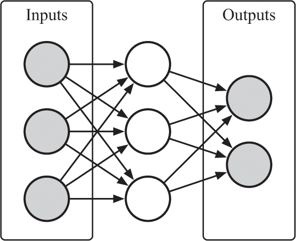
A simple neural network.
In that neural network diagram, each circle represents a neuron, and the arrows between neurons represent weights that describe the relationships between neurons. You can think of each neuron in the network as a little light bulb that is either on or off, depending on whether or not it is “activated.” If it is activated, it can take a range of numerical values. It may glow very dimly, or it may be extraordinarily bright. If it is not activated, it will not glow at all. Whether each neuron is off or on—and, if it is on, how brightly it glows—depends on the brightness of the neurons that feed into it and the weights that connect those neurons to this one.
The greater the weight between a neuron pair, the greater the influence of the upstream neuron on the downstream one. If the weights between neurons are negative, a brightly glowing neuron will inhibit the brightness of the neuron it points to.
You can see how the value of a neuron depends on the values of upstream neurons in figure 8.2. You’ll probably recognize immediately that this diagram is familiar: each neuron is just a simple weighted-average classifier with some function that squashes the output of the classifier in some way. In other words, the entire neural network is just a bunch of little classifiers wired together.
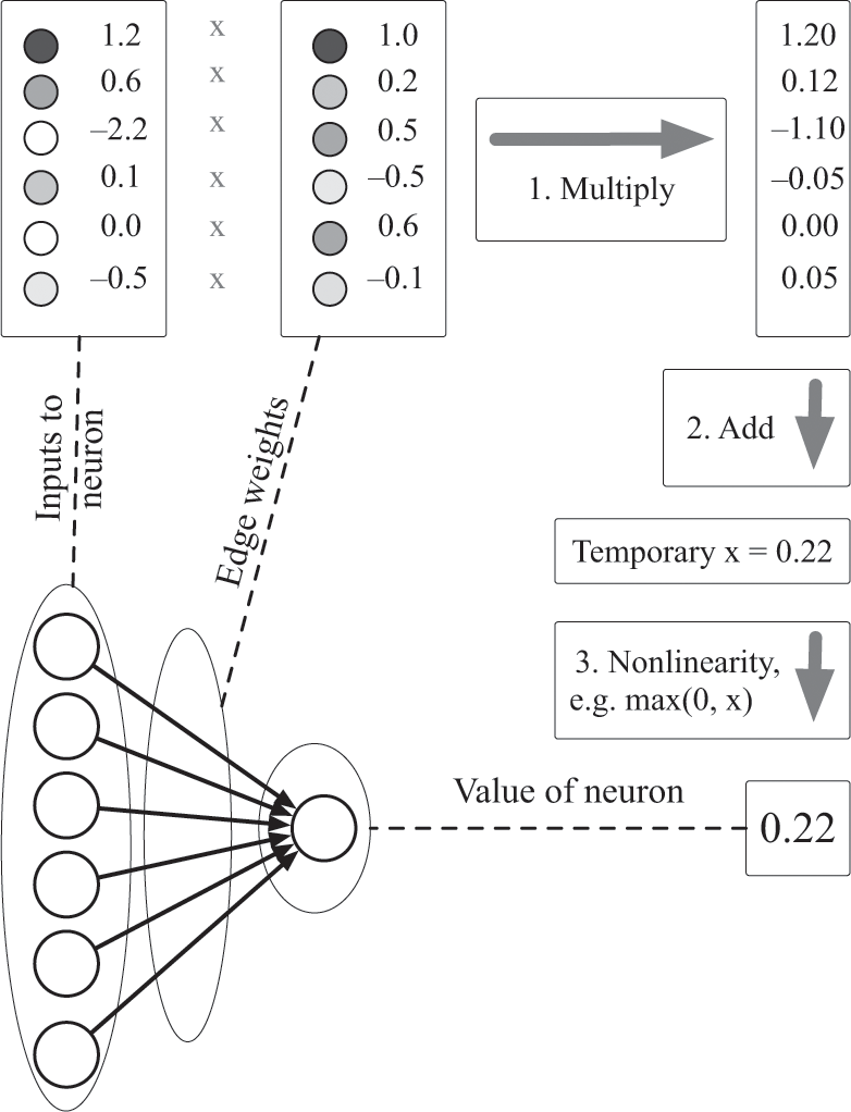
Propagation of values through a neural network. In neural networks, the value of a neuron is either specified by outside data—that is, it’s an “input” neuron—or it is a function of other “upstream” neurons that act as inputs to it. When the value of the neuron is determined by other neurons, the values of the upstream neurons are weighted by the edges, summed, and passed through a nonlinear function such as max(x,0), tanh(x), or an S-shaped function, exp(x)/(exp(x) + 1).
To use a neural network, we typically set the input neurons to specific values—for example, to match the colors of pixels in an image—three numbers in the range 0 to 1 for each pixel—and then we “run” the network. When we run it, the brightness of the neurons in the first layer will determine the brightness of neurons in the next layer, which will determine the brightness of neurons in the following layer, and so on, the information flowing through the network until it reaches the output layer. By the time the output neurons are activated, their values will hopefully be useful for some purpose. In the case of an Atari-playing agent, these neurons will tell us which action the agent should take.
Despite the biological inspiration for neural networks, there’s nothing mystical or mysterious about them. The brightness of the input neurons will determine precisely and unambiguously the brightness of the rest of the neurons in the network. Neural networks are just fancy calculators that evaluate a series of mathematical formulas; the connections between the neurons dictate, as in figure 8.2, what those formulas are. There’s no uncertainty, randomness, or magic in figuring out whether different neurons in the network will glow, as long as we know the weights of all of the connections between the neurons along with how the input neurons were set. A neural network is a computer, and it is therefore a prime building block for an automaton.
The network above is called a feedforward neural network, because information flows through it in a single direction, from the inputs to the outputs. In general, a neural network could have a different number of neurons in each layer, or it may have a different number of layers, or it may not even be organized into layers; but this feedforward architecture is still very common, and it’s what DeepMind used to play Atari games.
Let’s step back for a moment, though. Why bother using a neural network at all? Are we overcomplicating things? Could we design a simpler approximation to the q-function, maybe with just a simple classifier?
If our goal were to design an agent that played a single, specific game, the answer is probably yes. We could carefully handcraft features for the game and combine them with a weighted-average classifier. But doing so wouldn’t move us toward the goal of developing an automaton that can perform a wide variety of tasks, which was one of DeepMind’s goals in designing the Atari-playing agent in the first place. Remember: DeepMind’s agent could play about 50 different Atari games, many (but not all) of them very well, and DeepMind did no custom tuning for these games. It just let the agent play each game for a while. It needed a q-function that was flexible enough to play a wide variety of games.
It turns out that neural networks—even networks as simple as the one above—provide exactly the flexibility we need. An important theorem about neural networks, called the universal approximation theorem, states that if we were to use a network like the one above, with a single layer sandwiched between the input layer and the output layer, then we could approximate any function from the inputs to the outputs to any degree of accuracy.2 This is a profound theorem. It tells us that some neural network will indicate the best possible moves to make in an Atari game, given the pixels on the screen—provided that we select the network’s weights carefully. We just need to create the network to have the right shape and then find what those weights are, which brings us to the other major benefit of neural networks: their weights can easily be learned with data.
I show the universal approximation theorem in action in figure 8.3. First, look at the picture of the smiley face in figure 8.3a. This is a target we’d like to “predict” with a neural network. The remaining images in figure 8.3 show how well several neural networks with a single middle layer can approximate this target (the layers between the inputs and outputs are sometimes called “hidden” layers because we don’t directly observe their values. The input layer to each of these networks is two neurons, which are set to the x and y coordinates of each pixel in the image. The output of each network is a single neuron, which describes how dark the pixel at those coordinates should be: 0 for black and 1 for white. As we add more neurons to the middle—that is, the hidden—layer of the network, it can approximate its smiley-face target better and better. Figure 8.3c, which has 200 hidden neurons, somewhat resembles the face, while figure 8.3d, which has 2,000 hidden neurons, very much resembles the face.
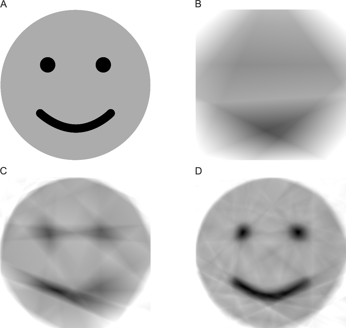
The performance of several neural networks (b)–(d) trained to represent a target image (a). The networks take as their inputs the x and y coordinates of each pixel in the image and predict the brightness of each pixel, in the range 0 to 1.
This network with a single hidden middle layer is the most “shallow” network we can use to still allow the network to represent arbitrary mappings from its input neurons to its output neurons. If we removed the middle layer and connected the input neurons directly to the output neurons, then the network wouldn’t be nearly as expressive. Our approximation to the smiley face would just be a gray box that gradually ranges from light gray to dark gray in some direction. We wouldn’t see eyes or a mouth. So we need at least one hidden layer between the inputs and the outputs.
The universal approximation theorem also doesn’t say anything about how big the middle layer of the network must be to approximate the smiley face as well as we’d like: we might need millions or billions of hidden neurons to represent the face beyond the limits of human perception, just as we might need millions of neurons in the hidden layer of a similar network to play Atari games. This observation is important to our goal of building an Atari-playing agent, because such a network might be too large to store on disk or too large to “train” with data, just as the original state-action cube was. This is the price we pay for trying to stuff all of this information into a single hidden layer. But it doesn’t mean that we can’t design a simpler network to play Atari in some other way—for example, by using more layers with fewer neurons per layer.
Before we build a network for the Atari agent, then, we need answers for two questions: What shape should we pick for the neural network? How do we select its weights? In the rest of this chapter I’ll answer these questions, and again we’ll again use the golf game to build the network.
THE ARCHITECTURE OF AN ATARI-PLAYING NEURAL NETWORK
In figure 8.4 I show a neural network designed to play the golf game. It has an input layer that takes the agent’s current position (x, y), an output layer that predicts in which of the eight directions the agent should aim, and a large hidden layer.
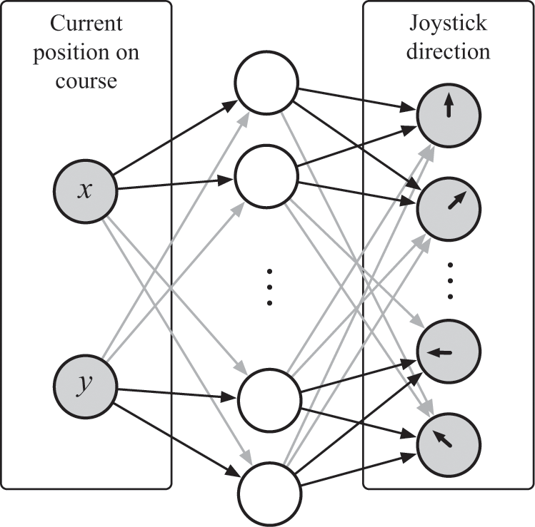
In this network, we will set the values of the input neurons so that they equal the coordinates of the current position of the ball using its position (x, y). When we run the network, the input neurons will activate the neurons in the middle hidden layer, and those neurons will then activate the output neurons. We want the output values of the network to approximate the values from the action-value cube we saw in the last chapter. Given the position of the ball, the output values of the network should be equal to the time-adjusted future rewards—that is, the amount of future chocolate—the agent should expect to receive for choosing that action. Once we’ve figured out this network’s weights, the agent will be able to choose its moves by setting the input neurons of the network with its position on the course, evaluating the network to produce values for its eight actions, selecting the action with the highest weight, performing that action, and then repeating this process.
As before, we just need to let the agent bumble around for a while so we can use its nuggets of experience to give the agent chocolate or an electric shock at the right times. I’ll explain in the next chapter how to “train” a neural network with data, but for now you just need to know that it’s possible to do this. We know that this architecture will work because the universal approximation theorem tells us that it will: we’ve already seen this with the smiley faces in figure 8.3. Because we’re starting with the coordinates (x, y), the network won’t need to be too large; it just needs to store eight different maps of where the agent should go—one for each output direction.
But wait—doesn’t the Atari-playing agent use raw pixel values instead of (x, y) coordinates as its input? I did kind-of cheat by letting our network take as its inputs the coordinates of the ball on the course instead of taking pixels representing the course. But it’s easy to get around this: we can do so by adding more layers at the beginning of this network to convert raw pixels into the coordinates of the ball on the course. This will be the last leap that will enable us to create neural networks that can play Atari games.
I’ve done this in figure 8.5. The right two layers in this network perform the exact same function we saw above, transforming the current position (x, y) into output values predicting chocolate yield; so we just need to convince ourselves that the left two layers can turn an image into the (x, y) coordinates of the golf ball.

A neural network designed to play the game golf. The right two layers, from the “Current position on course” to the “Joystick direction,” determine where the agent should aim, given the current position of the ball and the goal. The left two layers convert the pixels of the screen into the coordinates.
How could they do this? One way is to use a convolutional layer for the first hidden layer. A convolutional layer of a neural network contains classifiers that identify objects in the original input image, like the ball or the hole. Each classifier (we technically need only one in this case, to identify the ball’s position) is applied over every 8 × 8 patch of pixels in the input image. The output of this layer contains one image for each classifier. Each pixel of each output image is the result of applying the classifier over the respective patches in the input layer: black if there was no match with the classifier and white if there was a match.
You can see how this works for a single classifier in figure 8.6, which shows a convolution that uses 3 × 3 patches instead of 8 × 8 patches. In the figure, a classifier predicts whether each patch in the original image matches a certain pattern. The convolutional layer produces an image that aligns with the input image and describes where that image matches whatever the filter is looking for.
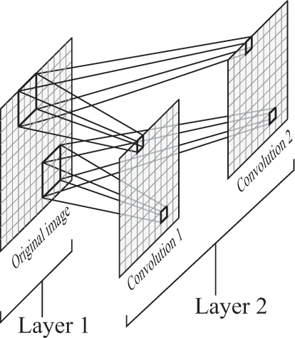
A convolutional layer with two filters. Each filter scans the image and produces a resulting image in which each “pixel” corresponds to a patch of the input image passed through that filter.
How do these classifiers work? Each classifier is just a weighted-average classifier like the one we used for the kids’ cookbook, possibly followed by a squashing function (more on this function in the next few pages). Remember: that’s all a neuron in a neural network is. Each pixel in the output of the convolutional layer is a neuron, where the weights correspond to the classifier’s weights.
To make things more concrete, let’s just assume that the golf course is a grayscale image, and that we’re using the original start-position of the ball and goal from the last chapter. The pictures in figures 8.7a and 8.7b show weights for classifiers that classify the flagpole and the ball from the original golf course in figure 7.2a. These filters will “activate”—that is, they will produce a value of 1—exactly when they are directly over the flagpole or the ball, respectively; otherwise they will produce a value of 0. If you squint a little, it’s clear that the filter in figure 8.7a looks a bit like the flagpole. The filter in 8.7b (for the ball) is less intuitive. It looks for lightly colored pixels surrounded by darker pixels, which is the defining characteristic of the ball.

Convolutional filters for the flagpole in the hole (left) and the ball (right).
The output of these convolutional filters is two images, each the result of applying one of the two classifiers over the original image, as you can see in figure 8.8. The output images are mostly black, except for one neuron in each that is glowing where the filter has found its pattern in the input image.
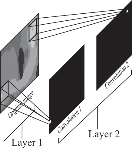
A convolutional layer with two filters. The filters are classifiers that scan the input image looking for certain patterns. The output of each filter is a set of neurons, organized as an image, which are “bright” wherever patches of pixels in the original image matched the filter.
To get from the second layer to the third layer, we simply need a mapping from each “pixel” in a black-and-white image to the coordinates (x, y) of the white pixel. The network has no idea that the pixel at one place in the image is adjacent to its neighbors: it just sees each image as big list of numbers. However, the network can learn the mapping from each pixel to its position by seeing enough data and encoding each neuron’s coordinates into the weights themselves, as shown in figure 8.9.
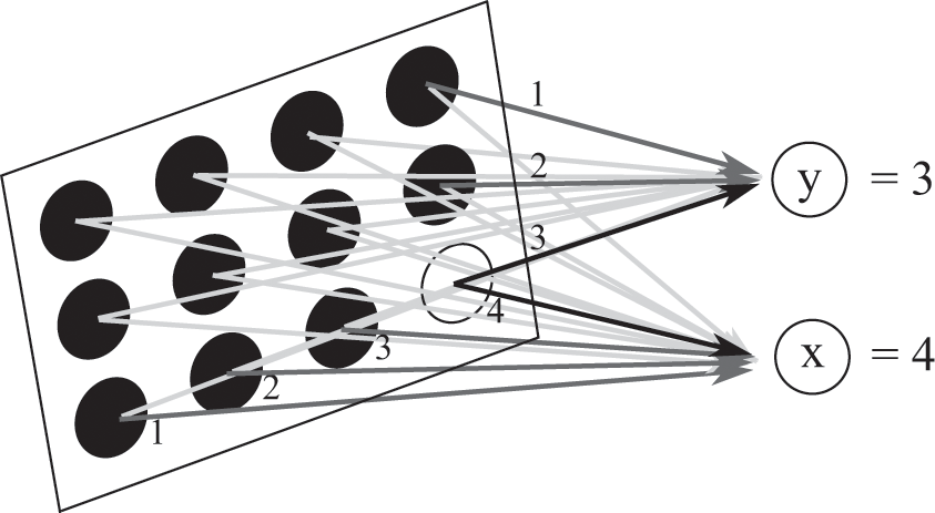
A layer that converts white pixels in a convolutional layer into coordinates. In this figure, the weight between a pixel and the neuron giving the x-coordinate is equal to the x-coordinate of that pixel, and the weight between a pixel and the neuron giving the y-coordinate is equal to the y-coordinate of the pixel. If the neuron at (4,3) in the left layer is glowing with a value of 1 and all other neurons are dark, then the values of the output of this layer will reflect this: they will be x=4 and y=3.
Now it turns out that this last step—that is, converting the output of the convolutional layer into coordinates—is useful for interpreting what’s happening in the network, but it’s not a necessary step for the network to work. Because we didn’t squash the neurons’ values after converting the position of the ball to its coordinates, it’s mathematically possible to fully connect the output of the convolutional layer to the final hidden layer before the output, and setting the weights to account for this. That lets us skip the middle layer that stores the (x, y) coordinates of the ball entirely.
And with this, we’ve constructed a network that is similar in spirit to the one used by the Atari-playing neural network. The first layer is a convolutional layer that looks for objects on the screen, squashing the result into the range 0 to 1. This layer is then fully connected to a hidden layer with 32 units, followed by another squashing function, and the result is fully connected to the output layer, the values of which represent the time-adjusted stream of chocolate the agent can expect to receive for taking different actions.
There are a few differences between this network and the one used by the Atari-playing agent. We used only two filters for the golf game (and we only needed to use one), but the Atari-playing agent used 32 separate filters in its first convolutional layer. The output of this first layer was then placed into 32 separate images, where each image glowed wherever the original image matched the respective filter. Since it had 32 filters, it could search for a wide variety of objects, from the paddle in the game Pong to the aliens or spaceships in Space Invaders. You can see an example of how it might apply this with several filters in figure 8.10.
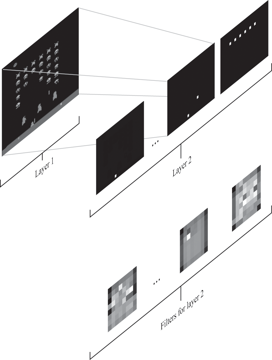
The convolutional layer of the Atari neural network. Layer 1 shows the input to the network: a screenshot of the game (the Atari network actually used 4 recent screenshots). The next layer is a convolutional layer that searches for 32 distinct patterns of pixels in the first layer with 32 filters. The result of applying each filter is 32 images, each of which is close to 0 everywhere except where the filter matches part of the input screenshot.
The Atari-playing network also had more convolutional layers than our golf network. The layers were stacked, so that the output of one layer was the input to the next layer. A later version of their network had three convolutional layers followed by the same two fully connected layers. By using three convolutional layers, their network could find more complex patterns of the input image. We’ll get some more intuition for why this can be useful in the next chapter, when we look at how deep neural networks can accurately interpret the content of photographs.
The architecture of this agent is somewhat reminiscent of the architectures in Stanley and Boss. You can compare the architecture of the Atari agent in figure 8.11 with Boss’s architecture, which was figure 4.2. An important part of those architectures was a separation of the components into a perception layer and a reasoning layer. The “perception” part of the Atari agent is the neural network, which takes the raw pixels on the screen and transforms them into useful features about the world. The “reasoning” part of the Atari agent is nothing more than a program that continuously looks at the output values of the neural network and selects the action with the highest value. You might even interpret this action-selection loop as a very simple type of “search” algorithm, whose goal is to search for the best among eight actions.
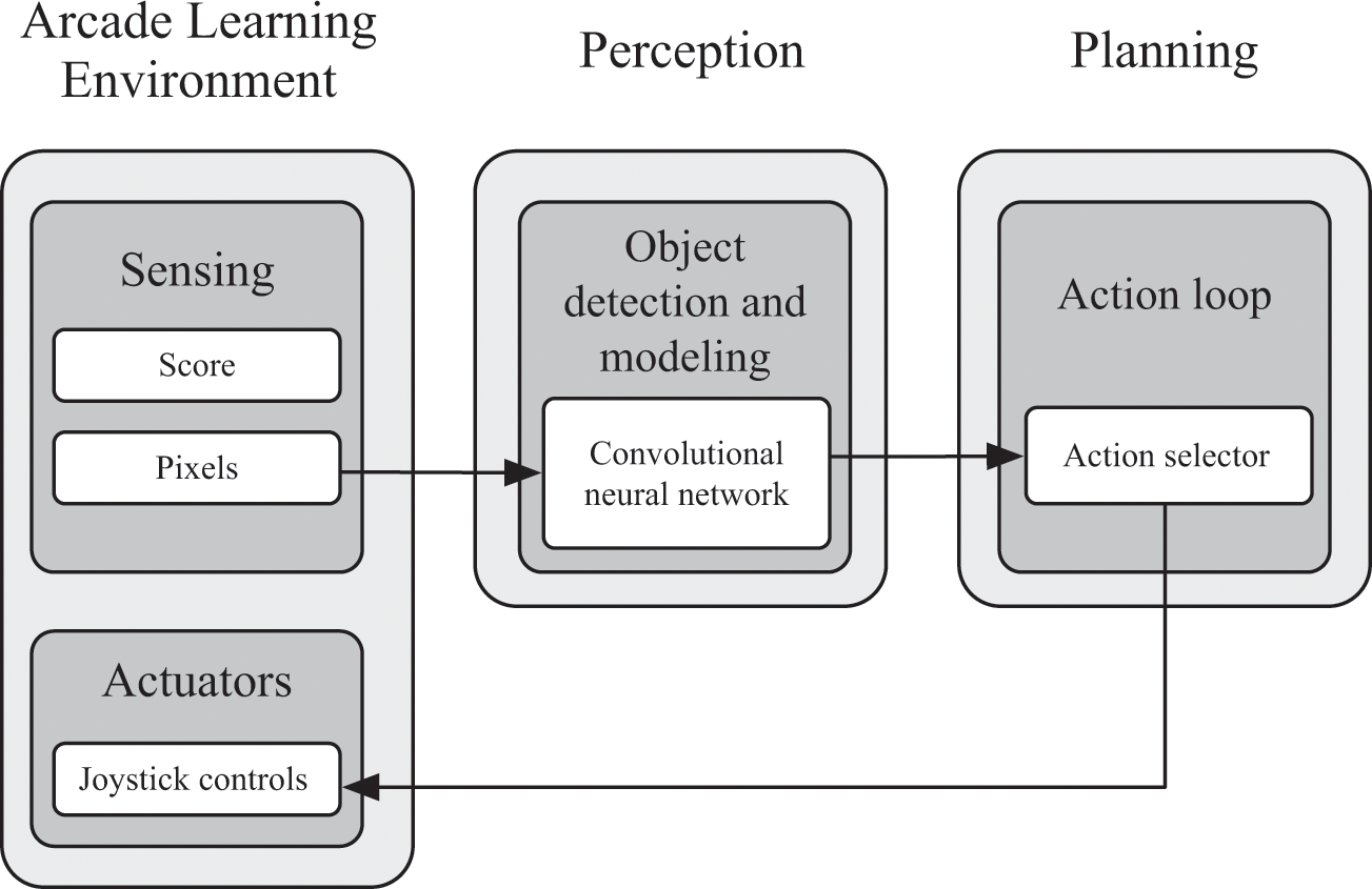
The architecture for an Atari-playing agent.
DIGGING DEEPER INTO NEURAL NETWORKS
Atari was in many ways a perfect testbed for DeepMind to demonstrate the strengths of neural networks. Atari games provided an explicit objective function for the agent—the number of points it had scored—while simultaneously offering a virtually unlimited amount of data for DeepMind to train its networks. Since the University of Alberta researchers had developed the Arcade Learning Environment, DeepMind could focus solely on the task of developing an agent that could play many games, exactly as the creators of the learning environment had intended. As we’ll see in chapter 9, quantity of data is one of the most important factors allowing us to train complex neural networks.
We’ve seen, at least at a high level, what happens in the neural network as it plays an Atari game. But many questions remain unanswered. For example, when does the Atari-playing agent not perform well? Although the agent used the same neural network architecture—that is, three convolutional layers followed by two fully connected layers—for each game, it learned different network weights for each game it played. After training, it played 29 of these games better than professional human players could play them.
The neural network performed best relative to humans on the Atari game Video Pinball. In pinball, the most important task of the agent is to react to a relatively small part of the game: where the pins hit the ball. The network simply needs to react, quickly and precisely, when the ball is near the bottom of the screen. The game also allows the player to “tilt” the pinball machine in either direction to nudge the ball to a better position. The agent could use this tilt operation to position the ball perfectly as it approaches the bottom of the screen. Since the network could learn about motion, and since it could react with machine precision, it earned about 20 times more points than professional human players at the game.3
The agent performed terribly on the game Montezuma’s Revenge.4 In Montezuma’s Revenge, the player is expected to explore a labyrinthine underground Aztec pyramid (think of Super Mario Brothers with ladders). The player moves from room to room while avoiding enemies and searching for jewels. The second-most-difficult game for the agent was a game called Private Eye, in which the player must search for clues and items throughout a city.
Both of these games involve exploration, which requires the player to maintain context throughout the game. The player must keep track of what it has done and what it hasn’t done, where it has gone and where it needs to go next. The Atari-playing agent couldn’t do this because it had no memory. It had no way to keep track of which rooms it had visited and which it hadn’t visited, of what it had done and what it hadn’t done.
There was also another, related reason it couldn’t play these games well. Remember that the agent initially trained itself by choosing completely random actions. By taking random actions, the agent couldn’t make much progress in games that required exploration. In Montezuma’s Revenge, the agent just stepped and bounced around the room, rarely if ever making it past the first room of the labyrinth. Because it couldn’t make much progress in its exploration, it couldn’t earn enough points to learn anything useful. Later we’ll see some ways agents can keep track of game state, but I’ll warn you now that we won’t get all of the answers we need: this is still an open problem and an active area of research for reinforcement-learning researchers.
One of the more successful parts of the Atari agent was its ability to perceive its world with convolutional neural networks. While relatively new, deep convolutional networks have quickly matured in the past few years, to the extent that computers can now classify objects in photographs better than many humans. In the next few chapters, we’ll take a look under the hood of some of these networks to see get a better sense for how they can do this.