A great many electrical and mechanical systems encountered in practice consist of many identical component parts. Such problems as the determination of the potential and current distribution along an electrical network of the ladder type or the determination of the natural frequencies of the torsional oscillations of systems consisting of identical disks attached to each other by identical lengths of shafting may be most simply solved by the use of difference equations.
The calculus of finite differences is of extreme importance in the theory of interpolation and numerical integration and differentiation. In this chapter some of the elementary procedures of the calculus of finite differences will be considered, and methods for the solution of linear difference equations will be developed.
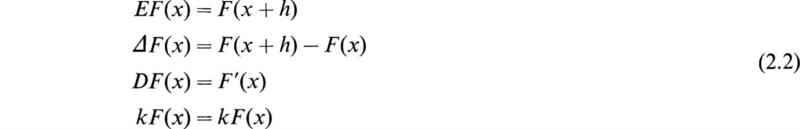
The calculus of finite differences is greatly facilitated by the use of certain operators. An operator may be defined as a symbol placed before a function to indicate the application of some process to the function to produce a new function. The symbol D = d/dx is an example; we have
In the calculus of finite differences it is convenient to use the operators E, ∆, D, and k, any constant. These operators indicate the following processes:
The operator E when applied to a function means that the function is to be replaced by its value h units to the right, D indicates differentiation, and the constant operator k merely multiplies the function by a given constant.
If now an operator is applied to a function and a second operator is applied to the resulting function, etc., the several operators are written as a product. Each new operator is written to the left of those preceding it. It may be shown that the order in which the operators are applied is immaterial. For example,
If an operator is repeated n times, this is indicated by an exponent. For example,
In this manner all positive and integral powers of operators may be defined. An operator with power zero produces no change in the function; for example,
Products of powers of operators combine according to the law of exponents; that is,
At present we shall restrict the powers of D and ∆ to be integral and nonnegative numbers. However, all real powers of E may be admitted. The general power of E is defined by the equation
These powers combine according to the law of exponents:
The sum or difference of two operators applied to a function is defined to be the sum or difference of the functions resulting from the application of each operator; that is,
In the above section the definitions of the operators E, ∆, D, and k were given. The meaning of all operators found from E, ∆, D, and k was given. The meaning of all operators found from E, ∆, D, and k by addition, subtraction, and multiplication was given. The question of separating these operators from the functions to which they apply and working with them as if they were algebraic quantities will now be considered.
Two operators are said to be equal if, when applied to an arbitrary function, they produce the same results. For example,
These operators, which we may call A, B, C, etc., may be combined as if they were algebraic quantities provided they conform to the following five laws of algebra:
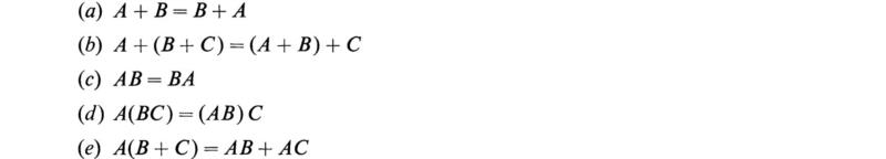
It is easy to show that the operators satisfy these fundamental laws of algebra. For example, to prove that
Since the operators satisfy the laws of algebra, operators can be combined according to the usual algebraic rules. For example,
etc.
As a consequence of the definition of the operators E and ∆, we have
The connection between the operator E and the derivative operator D may be obtained by means of the symbolic form of Taylor’s series given in Appendix C, Sec. 16. We see there that Taylor’s expansion could be written in the form
Comparing both members of Eq. (4.2), we see that we may write symbolically
We also have from (4.1)
or
If a function is known for equally spaced values of the argument, the differences of the various entries may be obtained by subtraction. It is very convenient to write these differences in tabular form. For example, let us consider the function F(x) = x3, and let the tabular difference be h = 1; we then construct the following table of differences:
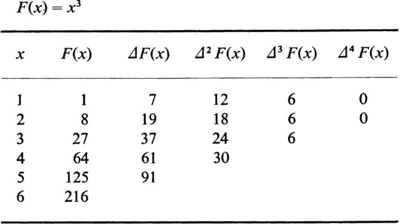
We see that the third differences of this function are constant and the fourth differences are zero. This is a special case of the following theorem:
The nth differences of a polynomial of nth degree are constant, and all higher differences are zero. The proof of this theorem is not difficult and is left as an exercise for the reader.
Difference tables are of extreme importance in the theory of interpolation. Interpolation in its most elementary aspects is sometimes described as “the science of reading between the lines of a mathematical table.” However, by the use of the theory of interpolation, it is possible to find the derivative and the integral of a function specified by a table taken between any limits. The utility of a difference table depends on the fact that in the case of practically all tabular functions the differences of a certain order are all zero.
Let us consider a function F(x) whose values at x = a, x = a + h, x = a + 2h, x = a + 3h, etc., are given. Suppose that from these given values of F(x) we construct a difference table and that the differences of order m are constant. We desire to compute the value of the function at some intermediate value of the argument a + nh. By the use of the operator E of Sec. 2 we have
By Eq. (4.1) we have
But, by the binomial theorem, we obtain
Hence we have from Eq. (6.1)
Now, in order to compute the value of F(x) corresponding to any intermediate value of the argument such as ![]() , we simply substitute the value of
, we simply substitute the value of ![]() in Eq. (6.4). Equation (6.4) is often referred to as Newton’s formula of interpolation. It was discovered by James Gregory in 1670.
in Eq. (6.4). Equation (6.4) is often referred to as Newton’s formula of interpolation. It was discovered by James Gregory in 1670.
From Eq. (4.5) giving the relation between the derivative operator D and the difference operator ∆, we have
Hence we have
If we expand ln(l + ∆) into a formal Maclaurin series in powers of ∆, we have
We thus have
for the derivative of the function F(x) at x = a.
To obtain higher derivatives, we have, from (7.2),
The second member is expanded and applied to F(a).
It is sometimes required to obtain the integral of a tabulated function over a certain range of the variable. To do this, it is convenient to introduce the operator D–1 or 1 / D. This operator is defined as the operator which when followed by D leaves the function unchanged; that is, we have
since if we operate on (8.1) with D, we obtain
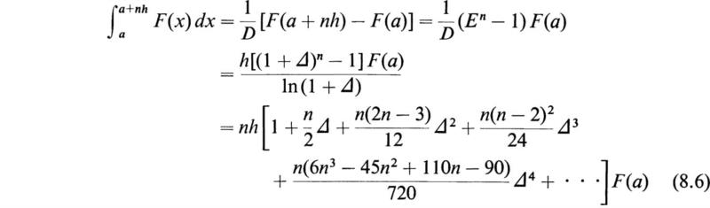
We also have the definite integral
If we use Eq. (7.2) for D, we may write (8.3) in the form
By division the right-hand member of (8.4) may be written in the form
By similar reasoning we have
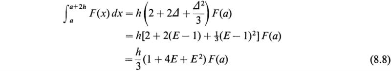
If n = 2, we have
If F(x) is such that its fourth and higher differences may be neglected, we have
This is known as Simpson’s rule for approximate integration.
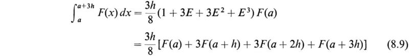
If F(x) is a polynomial of degree less than 4, formula (8.8) is exact. If we place n = 3 in (8.6) and neglect fourth and higher differences, we obtain
This is known as the three-eighths rule of Cotes.
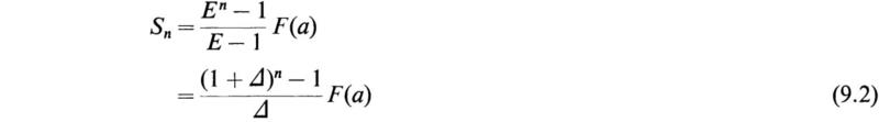
A formula of great utility for the summation of polynomials may be easily obtained by the use of the finite-difference operators. Consider the sum of n terms:
The geometric progression in E may be summed, and we have
Expanding (1 + ∆)n by the binomial theorem and dividing by ∆, we obtain
As an application of this equation, let it be required to find the sum of the first n cubes. To do this, we let F(x) = x3, h = 1, and we use the difference table of Sec. 5. We then have
The summation formula is exact if F(x) is a polynomial.
An equation relating an unknown function u(x) and its first n differences of the form
where the ar’s are constants, is called a linear difference equation of order n with constant coefficients.
This type of equation is of frequent occurrence in technical applications. It has many striking analogies with the linear differential equations discussed in Chap. 6. If ϕ(x) = 0, the equation is said to be homogeneous. By the use of the relation (3.1), Eq. (10.1) may be written in terms of the operator E in the form
where the b’s are constants. This is the form in which difference equations occur in practice.
As in the case of linear differential equations, the solution of the difference equation (10.2) consists of the sum of the particular integral and the complementary function. The complementary function is the solution of the homogeneous equation
In the usual applications of difference equations h = 1; that is,
etc.
To solve the homogeneous difference equation (10.3), we assume a solution of the exponential form
where c is an arbitrary constant and m is a number to be determined. If we operate on Eq. (10.5) with E, we obtain
In the same manner, we have
and in general
We therefore see that if we substitute the assumed solution (10.5) into the homogeneous difference equation (10.3), we obtain
If we let
Eq. (10.9) may be written in the form
If we exclude the trivial solution u(x) = 0, then
Hence the term in parentheses in (10.11) must vanish, and we have
This is an algebraic equation that determines the possible values of q. There are three cases to be considered.
a. The case of distinct real roots: If the algebraic equation (10.13) has n distinct roots (q1, q2,. . . , qn), then the general solution of the homogeneous difference equation (10.3) is
where the c’s are arbitrary constants.
For example, let it be required to solve the equation
In this case the algebraic equation determining the possible values of q is
The two roots of this equation are
Hence the solution of (10.15) is
where c1 and c2 are arbitrary constants.
b. The case of complex roots: Let us suppose that the algebraic equation (10.13) has pairs of conjugate complex roots. Let
be a pair of complex roots. The solutions of the difference equation corresponding to these terms are of the form
where A and B are two new arbitrary constants. As an example, consider the equation
Hence the solution of (10.21) is
where A and B are arbitrary constants.
c. The case of repeated roots: Suppose we have the difference equation
In this case the algebraic equation has repeated roots equal to a. To solve this equation, assume the solution
We now have
Similarly
Hence the function ![]() (x) satisfies the difference equation
(x) satisfies the difference equation
This equation is obviously satisfied by
where A and B are arbitrary constants. Hence the solution of (10.24) is given by
In the same manner it may be demonstrated that if the algebraic equation (10.13) has a root a that is repeated r times then the part of the solution due to this root has the form
where the c’s are arbitrary constants.
The difference equations most frequently encountered in practice are of the linear homogeneous type. The methods used for obtaining the particular integrals of linear differential equations with constant coefficients have their counterpart in the theory of difference equations. To illustrate the general procedure of determining the particular integral, let us write the linear inhomogeneous difference equation (10.2) in the form
where ![]() (E) denotes the linear operator involving the various powers of E expressed in Eq. (10.2).
(E) denotes the linear operator involving the various powers of E expressed in Eq. (10.2).
a. ϕ(x) is of the exponential form emx: In this case, to obtain the particular integral, assume the solution
where A is to be determined. On substituting this into (10.32) we have
Hence, provided that
we have
This case enables one to determine the solution when ϕ(x) is sin mx or cos mx by the use of Euler’s relation.
b. ϕ(x) is of the form ax: In this case we assume a solution of the form
On substituting this into (10.32) we obtain
Hence
provided that ![]() (a) ≠ 0.
(a) ≠ 0.
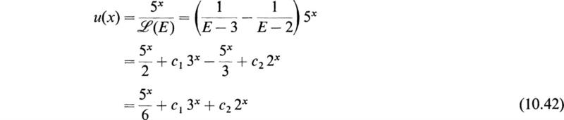
c. Decomposition of 1 / ![]() (E) into partial fractions: It is sometimes convenient to decompose the operator 1/
(E) into partial fractions: It is sometimes convenient to decompose the operator 1/ ![]() (E) into partial fractions. For example, consider the difference equation
(E) into partial fractions. For example, consider the difference equation
In this case the operator ![]() (E) has the factored form
(E) has the factored form
The decomposition of the operator 1/![]() (E) into partial fractions frequently facilitates the determination of the particular integral. Methods for the determination of the particular integral when ϕ(x) contains functions of special form will be found in the references at the end of the chapter.
(E) into partial fractions frequently facilitates the determination of the particular integral. Methods for the determination of the particular integral when ϕ(x) contains functions of special form will be found in the references at the end of the chapter.
The calculus of finite differences may be applied to the solution of dynamical problems, whether electrical or mechanical. This calculus has great power when the system under consideration has a great many component parts arranged in some order. It may be that there are so many component parts that to write down all their equations of motion would be impossible. If there exists a certain amount of similarity between the successive component parts of the system, it may be possible to write down a few difference equations and in this manner include all the equations of motion. This may be illustrated by the following problem:
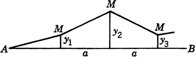
Consider a string of length (n + 1) a, whose mass may be neglected, which is stretched between two fixed points with a force τ and is loaded at intervals a with n equal masses M not under the influence of gravity, and which is slightly disturbed. Let it be required to determine the natural frequencies of the system and the modes of oscillation.
Let (A, B) (Fig. 11.1) be the fixed points and (y1, y2, , yn) be the ordinates at time t of the n particles. Consider small displacements only and hence the tensions of all the strings as equal to τ. The force on the kth mass is given by
Fig. 11.1
This is a restoring force acting in the negative direction. By Newton’s second law the equation of motion of the kth particle is given by
Since each particle is vibrating, let us place
Substituting this into (11.2) and dividing out the common cosine term, we obtain
If we let
we may write (11.4) in the convenient form
This is a homogeneous difference equation of the second order with constant coefficients in the unknown amplitude Ak. To solve it, we use the method of Sec. 10 and assume a solution of the form
where B is an arbitrary constant and θ is to be determined. If we substitute this assumed form of the solution into (11.6), we obtain
Therefore, for a nontrivial solution, we must have
This equation determines two values of θ since cosh θ is an even function, and we also have
Hence, B1eθk and B2e–θk are solutions of the difference equation (11.6), and the general solution is the sum of these two solutions. It is convenient to write the general solution in terms of hyperbolic functions rather than in terms of exponential functions. We thus write
where P and Q are arbitrary constants. Equation (11.2) represents the amplitude of the motion of every particle except the first and last. In order that it may represent these also, it is necessary to suppose that y0 and yn+1 are both zero, although there are no particles corresponding to the values of k equal to 0 and n + 1. With this understanding the solution (11.11) represents the amplitude of the oscillation of every particle from k = 1 to k = n. Now, since A0 = 0, we have from (11.11)
The fact that An+1 = 0 gives
This equation fixes the possible values of θ; they are
Having determined the possible values of θ , we now turn to Eq. (11.5) to determine the possible values of ω. We thus obtain
Hence
It is convenient to write ωr to denote the value of ω that corresponds to the number r. We thus write
The amplitude of the motion of each particle is given by Eq. (11.11) in the form
The amplitude of the motion of the first particle is given by
If, now, the value r = 0 were admitted, this would preclude the motion of the first particle. Similarly the value r = n + 1 is not admitted. The values of ω given by Eq. (11.17) are the n natural angular frequencies of the system. Giving r other values not multiples of n + 1, we merely repeat these frequencies. To each value θr of θ there corresponds a term of the amplitude of the kth particle. This may be written in the form
where ![]() is an arbitrary constant.
is an arbitrary constant.
By (11.3) the coordinate of the kth particle corresponding to the value θr of θ is given by
The general solution is then of the form
The 2n arbitrary constants ![]() and ϕr are determined by the initial displacements and velocities of the particles.
and ϕr are determined by the initial displacements and velocities of the particles.
The problem of the loaded string is of historical interest. It is discussed by Lagrange in his “Mécanique analytique.” He deduced the solution from his own equations of motion. By means of an extension of the above analysis Pupin treated the problem of the vibration of a heavy string loaded with beads, both for free and for forced vibrations, and by an electrical application solved a very important telephonic problem.†
The following interesting electrical problem may be solved by the use of difference equations.
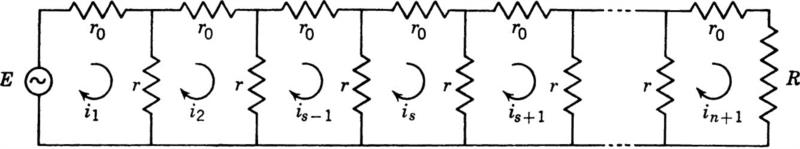
Let us suppose that the current for a load of resistance R is carried from the generator to the load by a single wire with an earth return. The wire is supported by n equally spaced identical insulators, as shown in Fig. 12.1.
Fig. 12.1
The resistance of the sections of wire between insulators is r0. The resistance of the earth return is negligible. Let us suppose that in dry weather when the insulators are perfect the current supplied by the generator is Id but in wet weather it is necessary to supply a current Iω in order to receive a current Id at the load R. Assuming that the leakage of all the insulators is the same, let it be required to find the resistance r of each.
If we write Kirchhoff’s second law for the sth loop, we obtain the difference equation
This may be written in the form
If we assume a solution of the form
where c is an arbitrary constant, and substitute this into the difference equation, we find that
The general solution of (12.2) may be written in the form
To determine the arbitrary constants A and B, we have for the current in the first loop
Also in the (n + l)st loop we have
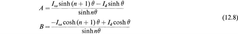
If we solve these two simultaneous equations for A and B, we obtain
Substituting these values for A and B into (12.5), we obtain
If we write Kirchhoff’s second law around the last loop, we obtain
If we solve Eq. (12.4) for r, we obtain
Substituting this value of r, and in from (12.9), into (12.10), we obtain after some reductions
This equation may be solved graphically for θ by the methods of Appendix D. Substituting the value of θ determined by this equation into Eq. (12.11) gives the desired value of r. If, as is usually the case, the line resistance r0 is small in comparison with the insulator resistance, that is, if
then we have
and we may make the approximation
realizing that if x is small we have
Using these approximations in Eq. (12.12) and solving for θ, we obtain
Hence
for the required value of r.
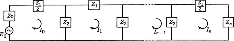
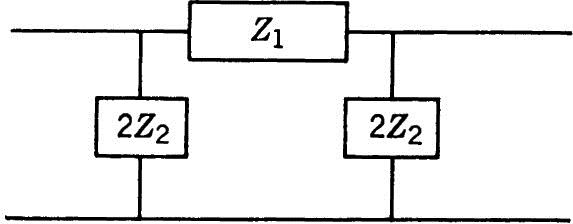
In Chap. 7 the mathematical technique for the determination of the steady-state behavior of alternating-current networks was explained. A very important type of network is one in which numbers of similar impedance elements are assembled to form a recurrent structure. Networks of this type are called filters because they pass certain frequencies freely and stop others. Various forms of structure may be employed. A very common structure is the so-called “ladder” structure. This is shown in Fig. 13.1.
Fig. 13.1
Except for the end meshes this structure consists of a number of identical series elements of complex impedance Z1 and a number of shunt elements of complex impedance Z2. The input and output impedances are Z0 and Zn, respectively, and there is a complex applied electromotive force
applied to the first mesh. The real and imaginary parts of this complex electromotive force correspond to actual electromotive forces of the type E0cos ωt or E0sin ωt. We assume that the instantaneous currents in the various meshes have the form
where the Is are the ordinary complex currents of steady-state alternating-current theory. The real or imaginary parts of (13.2) correspond to an applied potential of the form E0cos ωt or E0sin ωt, respectively, with proper phase.
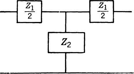
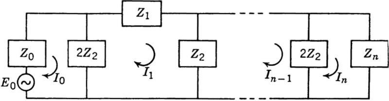
The circuit of Fig. 13.1 is composed of nT sections of the type shown in Fig. 13.2. As shown, the filter ends with half-series elements and is said to have mid-series terminations. It is sometimes more convenient to arrange the filter circuit as shown in Fig. 13.3. This circuit is said to have mid-shunt terminations. In this case we regard the filter as made up of n – 1 so-called “sections,” as shown in Fig. 13.4.
The type of termination affects the values of the currents in the different sections of the filter for given input and output impedances. However, it
Fig. 13.2
Fig. 13.3
Fig. 13.4
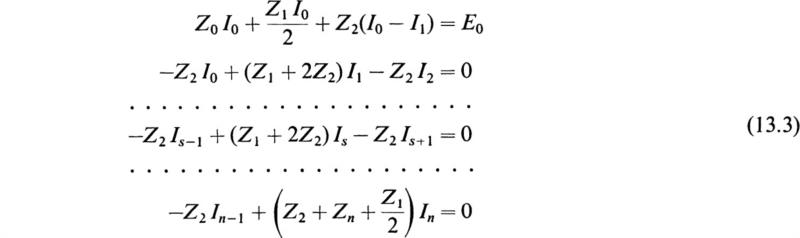
does not affect the frequency characteristics of the filter. It is therefore necessary to analyze only one case, and we shall choose the case of the mid-series termination. If we apply Kirchhoff’s second law to the various meshes of Fig. 13.1, we obtain the following set of equations:
The equation for the sth mesh may be written in the form
This difference equation has a general solution of the form
where A and B are arbitrary constants. The number a is given by
The quantity a is, in general, complex and is called the propagation constant of the filter. Since a is complex, let us write
The actual instantaneous current is(t) is obtained by multiplying the complex amplitude Is by ejωt in the form
Assuming that α > 0, we thus see that there is an attenuation factor e–α introduced into the amplitude of the first term by each section of the filter as we move away from the input end. Similarly, for the second term of (13.8), there is an attenuation for each section of the same amount as we move toward the input end. It is thus apparent that if α differs from zero for any frequency and the filter has an appreciable number of sections the current transmitted by the filter is effectively zero. On the other hand a current whose frequency is such that α = 0 is freely transmitted. The quantity α is called the attenuation constant.
In the same manner ϕ is called the phase constant since it gives the change of phase per section (measured as a lag) in the currents as we move along the filter.
The physical significance of Eq. (13.8) is now clear. The first term represents a space wave of current traveling away from the input end, attenuated from section to section much as the time waves of the free oscillations of a circuit are attenuated from instant to instant. The second term represents a similar wave traveling back toward the input end, arising from reflection at the output end.
From Eq. (13.8) we see that there are two separate points of interest to be considered:
1. The dependence of the frequency characteristics upon the filter construction, that is, on the nature of Z1 and Z2.
2. The dependence of the transmission characteristics upon the terminating impedances Z0 and Zn.
The first matter involves only Eqs. (13.6) and (13.7), while the second matter involves the determination of the arbitrary constants A and B.
If the resistances of the elements Z1and Z2 of the filter are so small that they may be neglected, then Z1 and Z2 are pure imaginary quantities. It follows, therefore, that
is real.
If we now express cosh a in terms of α and ϕ, we have
Now since cosh a is real, either α must be zero or ϕ must be an integral multiple of π. Hence, since cosh α is never less than unity and cos ϕ is never greater than unity, we have three cases to consider.
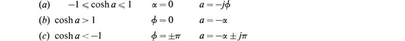
In the frequency range corresponding to case a, currents are transmitted freely without attenuation. The range of frequencies for which this is the case is called a passband. Frequency ranges corresponding to the other two cases are called stopbands.
In terms of Z1 and Z2, the passbands are given by
or
Stopbands are given by all other ranges of values.
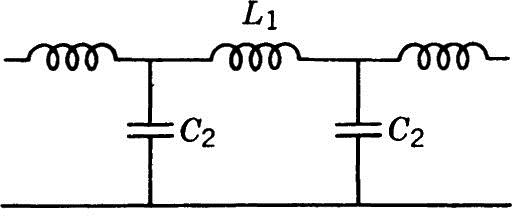
The simplest filters of the types we are considering are given by Figs. 13.5 and 13.6. For the arrangement of Fig. 13.5, we have
The passband is given by
or
Fig. 13.5
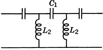
Fig. 13.6
Since all frequencies from 0 to a critical, or cutoff, frequency given by
![]()
are passed without attenuation, we have a low-pass filter.
In the arrangement of Fig. 13.6 we have
The passband is now determined by
or
Here all frequencies above a critical frequency are passed without attenuation. This arrangement is called a high-pass filter. More complicated arrangements may be treated in a similar manner.
The values of the arbitrary constants A and B of the solution of the difference equation (13.5) are most simply expressed in terms of the characteristic impedance Zk of the given filter.
By definition the characteristic impedance of a filter of the type we are considering is the input impedance of the filter when it has an infinite number of sections. It is evident that, in this case, the wave due to reflection at the output end, which is represented by the second term of (13.5), vanishes. The current in each section is now independent of the terminal impedance Zn, and the general solution (13.5) reduces to
If s = 0, we have
Hence we may write
The first of Eqs. (13.3) now becomes
But by definition, since Zk is the impedance at the sending end of the entire filter that has an infinite number of sections, we have
Comparing Eqs. (13.22) and (13.23) and using (13.9), we have
If we square this equation and use Eq. (13.6), we obtain
Hence, finally,
We can show that when we neglect the resistance parts of Z1 and Z2 then Zk is real in the passbands and imaginary in the stopbands.
To determine the constants A and B for the actual filter with a finite number of sections, we substitute (13.5) in the first and last of the equations of (13.3). We then obtain
However, from Eq. (13.24) we have
and, similarly,
Hence Eqs. (13.27) may be written in the convenient form
Solving these simultaneous equations for A and B and substituting the result into (13.5), we obtain
where
The quantities rs and rR are called the sending-end and receiving-end reflection coefficients, respectively.
If the output impedance matches the characteristic impedance of the line, then
Under this condition the filter with its terminating impedance behaves like an infinite filter. The reflection coefficient rR = 0, and reflection is absent. In this case all the energy delivered to the filter at the input end is transmitted to Zn, and the filter operates at maximum efficiency. In this case Eq. (13.31) reduces to
In practice, one is more interested in the input and output currents than in the intermediate currents. The completeness of filtering is measured by the ratio
In this section it will be shown that there exists an intimate connection between difference equations and matrix multiplication. To fix the ideas, we shall consider an application to electrical-circuit theory, and we shall see that in certain cases matrix multiplication has some advantages over the method of difference equations in that we need not solve for the arbitrary constants that appear in the solutions of the difference equations.
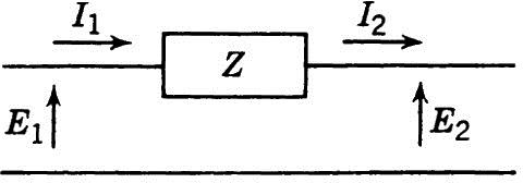
Consider the electrical circuit of Fig. 14.1. This circuit consists of a series impedance and a perfect conductor return path. We suppose that an electromotive force
Fig. 14.1
Fig. 14.2
is impressed on one end of the circuit and that an electromotive force
is impressed on the other end of the circuit. This gives rise to a current
Since we are interested in steady-state values, we may suppress the factor ejωt as is customary in electrical-circuit theory. We then concern ourselves only with the complex amplitudes E1, E2, I1, and I2. By Kirchhoff’s laws, we have the relations
This may be written in the convenient matrix form
This matrix equation expresses a relation between the input quantities E1 and I1 and the output quantities E2 and I2. We notice that the determinant of the square matrix of (14.5) is equal to unity.
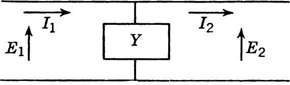
Let us now consider the circuit of Fig. 14.2. By Kirchhoff’s laws, we now have the relations
where Y is the admittance of the circuit and is hence the reciprocal of the impedance. This relation may be written in the matrix form
We notice that, in this case also, the determinant of the square matrix is equal to unity.
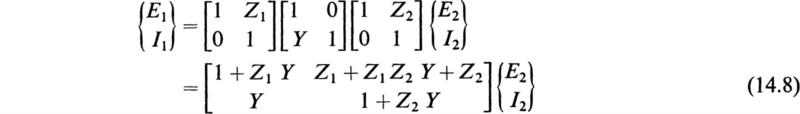
Let us now consider the network of Fig. 14.3. We may regard this circuit as being formed by a circuit of the type of Fig. 14.1 in series with a circuit of the type of Fig. 14.2 and another circuit of the type of Fig. 14.1.
Fig. 14.3
Fig. 14.4
Since the output currents and voltage of one circuit are the input currents and voltages of the next network, we obtain
We thus may obtain the input and output quantities directly. The elements of the square matrix are functions of the impedances and admittances of the component parts of the network. Since the square matrix of (14.8) is the product of three matrices whose determinants are each equal to unity, its determinant also is equal to unity. The square matrix of Eq. (14.8) is called the associated matrix of the network.
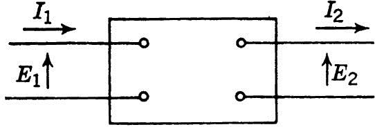
Let us consider a box with four accessible terminals as shown in Fig. 14.4. Let us assume that within the box there exist various impedance and admittance elements joined together in a general manner. Let us also assume that there are no potential sources within the box. It may then be shown by a repeated multiplication of the associated matrices of the individual elements within the box that the input and output potentials and currents are related by the equation
where in general A, B, C, D are complex numbers and the determinant of the square matrix of (14.9) satisfies the relation
If we premultiply both sides of Eq. (14.9) by
![]()
we obtain
If the network within the box is symmetrical so that it appears the same when viewed from the right as when viewed from the left, we have
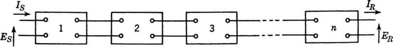
Let us suppose that we have a chain of n identical symmetrical networks connected as shown in Fig. 14.5. Since the networks are identical and symmetrical, we have the relation
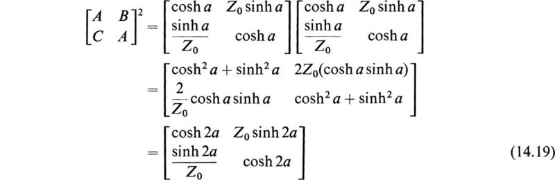
There exists a very convenient manner of writing the matrix
![]()
to enable one to raise it to a positive or negative integral power. To do this, we let
Now since the determinant of
![]()
equals unity, we have
or
Hence with these substitutions we write
Fig. 14.5
By mathematical induction it may be shown that
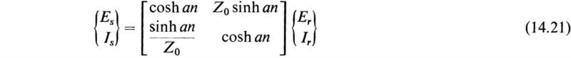
The result (14.20) holds for n a positive or negative integer. We therefore have
This gives the relation between the receiving-end quantities and the sending-end quantities. If we premultiply Eq. (14.13) by

we obtain
Expressions (14.21) and (14.22) are extremely useful in the field of electrical-circuit theory, and, by the electrical and mechanical analogues, they are of use in the field of mechanical oscillations.
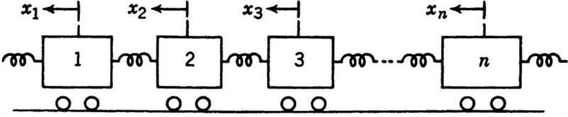
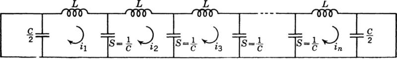
As a simple mechanical example of the above general theory, let us consider the longitudinal motions of a train of n equal units as shown in Fig. 15.1. For simplicity we shall assume that the mass of each unit is m and that the units are coupled together by coupling whose spring constant equals k. Friction will be neglected.
Fig. 15.1
Fig. 15.2
By the principles explained in Chap. 6, the mechanical system of Fig. 15.1 is analogous to the electrical system of Fig. 15.2. This is a ladder network having n meshes. By the electrical-mechanical analogy principle, we have the following analogous quantities:
where L is the inductance parameter of each mesh of the ladder network, S is the elastance of each capacitor of the network, ir is the mesh current of the rth mesh, qr is the mesh charge, xr is the coordinate of the rth unit of the train, and υr is the velocity of the rth unit.
The electrical circuit may be regarded as being composed of n units of the π type as shown in Fig. 15.3. The associated matrix of the circuit of Fig. 15.3 is
Fig. 15.3
We now let
in accordance with Eqs. (14.14) and (14.15).
We may then write the associated matrix of the circuit (15.5) in the form
To obtain the natural frequencies of the dynamical system of Fig. 15.1, we realize that when the train is oscillating freely there are no external forces exerted upon it at either end. Hence, in the equivalent electrical circuit, the sending-end and receiving-end potentials must be equal to zero. We thus have
Since Es = 0, we have
where Is is arbitrary. The frequency equation of the system is therefore given by
If, in Eq. (15.6), we let
and solve for ω, we find
If we now substitute this into (15.7), we have
The frequency equation (15.11) then becomes
This equation is satisfied if
or
Substituting this into (15.13), we obtain the n natural angular frequencie ωr :
Translating this result into mechanical language, we obtain
for the natural angular frequencies of oscillation of the train of n units.
1. Find the successive differences of F(x) = 1/x, the interval h being unity.
![]()
by integrating numerically.
3. A curve expressed by F(x) has for x = 0, 1, 2, 3, 4, 5, 6 the ordinates 0, 1.17, 2.13, 2.68, 2.62, 1.77, –0.07, respectively. Find the slope of the curve at each of the seven points, and find the area under the curve from x = 0 to x = 6.
4. Show that l4 + 24 + 34 + + n4 = (n/30)(6n4 + 15n3 + 10n2 – 1).
![]()
6. Sum, to m terms, the series
![]()
Solve the following difference equations:
7. u(x + 2) – 3u(x + 1) – 4u(x) = m*.
8. u(x + 2) + 4u(x + 1) + 4 = x.
9. ∆u(x) + ∆2 u(x) = sin x.
10. u(x + 2) + n2 u(x) = cos mx.
11. A seed is planted. When it is one year old, it produces tenfold, and when two years old and upward, it produces eighteenfold. Every seed is planted as soon as produced. Find the number of grains at the end of the xth year.
12. A low-pass filter with mid-series termination is constructed of elements L1 = 1/π henry, C2 = 1/ π μf. Find the cutoff frequency.
13. Draw the equivalent electrical circuit for the loaded string. Use the matrix method to compute the natural frequencies of the system.
14. Consider an infinitely extended string under tension F. The string carries equal equidistant masses m and is immersed in a viscous fluid. Draw the equivalent electrical circuit, and discuss the nature of wave propagation when a harmonic transverse force is impressed on the first mass.
15. A shaft of constant cross section carries n identical disks spaced at equal intervals of length a. The moment of inertia of each disk is denoted by J. The torsional stiffness of each section of shaft between two disks is determined by the constant c such that if the relative angular displacement of two neighboring disks is equal to θ, the torque transmitted by the section is equal to cθ. Determine the natural frequencies of the torsional oscillations of the system. If an oscillatory torque is applied to the first disk, determine the motion of the last disk.
16. A transmission-line conductor carries an alternating current of angular frequency ω. It is supported by a string insulator of n identical units attached to a metallic transmission-line tower that is at zero potential. Assume that the metallic conductors between two insulators form an electrical capacitor of capacitance c1; also, each metallic conductor and the tower form a capacitor of capacitance c2. Determine the potential distribution along the chain of insulators.
17. A light elastic string of length ns and coefficient of elasticity E is loaded with n particles each of mass m ranged at intervals s along it, beginning at one extremity. If it is suspended by the other end, prove that the periods of its vertical oscillations are given by the formula
![]()
18. A railway engine is drawing a train of equal carriages connected by spring couplings of strength y, and the driving power is adjusted so that the velocity is A + Bsinqt. Show that, if q2[(M + 4m)b2 + 4mk2] is nearly equal to 2μb2, the couplings will probably break. M is the mass of a carriage that is supported on four equal wheels of mass m, radius b, and radius of gyration k. Are there any other values of q for which the couplings will probably break ?
19. A regular polygon A1 A2, . . . , An is formed of n pieces of uniform wire, each of resistance r, and the center 0 is joined to each angular point by a straight piece of the same wire. Show that, if the point 0 is maintained at zero potential and the point A1 at potential V, the current that flows in the conductor As, As+1 is
![]()
Where θ is given by the equation cosh2θ = 1 + sin(π/n).
1880. Boole, George: “A Treatise on the Calculus of Finite Differences, ” The Macmillan Company, New York.
1905. Routh, E. J.: “Advanced Rigid Dynamics,” The Macmillan Company, New York.
1920. Funk, P.: “Die Linearen Differenzengleichungen und ihre Anwendungen in der Theorie der Baukonstruktionen, ” Springer-Verlag OHG, Berlin.
1940. Kármán, T. V., and M. A. Biot: “Mathematical Methods in Engineering,” McGraw-Hill Book Company, New York.
† M. Pupin, Wave Propagation over Non-uniform Electrical Conductors, Transactions of the American Mathematical Society, vol. 1, p. 259, 1900.