One of the most important and interesting subjects of applied mathematics is the theory of small oscillations of mechanical systems in the neighborhood of an equilibrium position or a state of uniform motion. In the last chapter we considered the oscillations of a very important vibrating system, the electrical circuit. By the analogy between electrical and mechanical systems all the methods discussed in the last chapter may be used in the analysis of mechanical systems. In the mechanical system we are usually concerned with the determination of the natural frequencies and modes of oscillation rather than the complete solution for the amplitudes subject to the initial conditions of the system. In this chapter we shall use the classical method of solution rather than the Laplace-transform method. By comparing the analysis of the equivalent electrical circuits of the last chapter which were analyzed by the Laplacian-transformation method and the classical analysis of the mechanical systems in this chapter, a proper perspective of the utility of the two methods will be apparent.
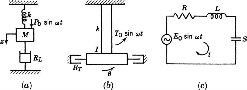
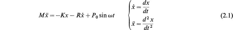
Let us consider the vibrating systems of Fig. 2.1. System a represents a mass that is constrained to move in a linear path. It is attached to a spring of spring constant k and is acted upon by a dashpot mechanism that introduces a frictional constraint proportional to the velocity of the mass. The mass has exerted upon it an external force P0 sin ωt. By Newton’s law we have
where K is the spring constant and R is the friction coefficient of the dashpot.
System b represents a system undergoing torsional oscillations. It consists of a massive disk of moment of inertia j attached to a shaft of torsional stiffness K. The disk undergoes torsional damping proportional to its angular velocity θ. The disk has exerted upon it an oscillatory torque T0 sinθt. By Newton’s law we have
System c is a series electrical circuit having inductance, resistance, and elastance. By Kirchhoff’s law the equation satisfied by the mesh charge q is
Fig. 2.1
By comparing these three equations, we obtain the following table of analogues:

We see from this table of analogues that it is necessary only for us to analyze one system and then by means of the table we may obtain the corresponding solution for the others.
Let us consider the system a when no impressed force is present. In this case, Eq. (2.1) reduces to
This equation describes the free vibrations of the mass of Fig. 2.1. To find the general solution of (2.4), we find two nontrivial solutions. An arbitrary linear combination of the two particular solutions will then be the desired solution.
Since Eq. (2.4) is linear and homogeneous, we know from the general theory of Chap. 2 that we can obtain a particular solution of the form est where s is a constant to be determined. If we substitute est for x in (2.4) and divide out the factor est, we obtain the quadratic equation
This equation determines the quantity s. Let us denote the two roots of the quadratic equation (2.5) by s1 and s2. We then have
for the general solution of (2.5), where c1 and c2 are arbitrary constants. The nature of the solution depends on the nature of the roots. There are three cases to consider.
a. The case R2 - 4MK> 0: In this case s1 and s2 are real and unequal. The general solution is
Both roots are negative, and (2.7) represents a disturbance that vanishes as t approaches infinity.
b. The case R2 - 4MK=0: In this case the quadratic equation (2.5) has a double root
Thus c1e(–R/2M)t is the only solution obtainable from (2.5). However, the general theory of repeated roots as discussed in Chap. 2 shows that there exists a second solution of the form x = te(–R/2M)t. The general solution is therefore
In both these cases we have the so-called “aperiodic motion.” As time increases, the displacement of the mass approaches zero asymptotically without oscillating about x = 0. This means that the effect of damping is so great that it prevents the elastic force from setting up oscillatory motions.
c. The case R2 – 4MK < 0: In this case, the roots s1 and s2 are complex conjugates. If we let
we may write the general solution in the form
By using the Euler relation, this becomes
where ć1 and ć2 are two new arbitrary constants. If we let
where A and δ are two new arbitrary constants, the (2.12) becomes
The constant A is called the amplitude of the motion, and ωsδ is called the phase,
is called the angular frequency of the motion. The motion represented by (2.14) is quite different from the aperiodic motion discussed in cases a and b. In this case the damping is small compared with the elastic force, and the motion of the mass is oscillatory. The damping is not so small as to be considered negligible. The motion is one of damped harmonic oscillations. The oscillations behave like cosine waves with an angular frequency of ωs except that the maximum value of the displacement attained with each oscillation is not constant. The “amplitude” is given by the expression Ae(–R/2M)t and decreases exponentially as t increases.
The quantity R/2M is called the logarithmic decrement. It indicates that the logarithm of the maximum displacement decreases at the rate R/2M. If there is no damping present (R = 0), we obtain harmonic oscillations with natural angular frequency
The amplitude A and the phase ωsδ must be determined from the initial state of the system. If, for example,
then
is the particular solution.
If an external force F(t) is impressed upon the physical system a above, the equation governing the displacement x of the mass is given by
From the general theory of Chap. 2 we know that the general solution of (2.19) is the superposition of the general solution of the homogeneous equation (2.4) and the particular solution of (2.19). Let the force (Ft) be a periodic force of the form
Accordingly we have
Since this equation is linear, we attempt to find a solution of the form
We realize that the real part of the solution corresponds to the force function F0cosωt and the imaginary part of the force function F0sinωt. Substituting the assumed form of the solution in Eq. (2.21), we obtain
or
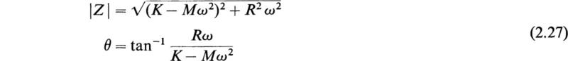
The complex number
may be written in the polar form
where
We then have
Substituting this into Eq. (2.22), we have
The physical meaning of this solution is that if a force of the form F0cosωt is impressed on the vibrating system, the resulting steady-state motion is given by
If a force F0sinωt is impressed on the system, then the steady-state response is
The complex number Z is called the mechanical impedance of the system. It is a generalization of the spring constant to the case of oscillatory motion. It is convenient to introduce the quantity μ, defined by
μ is called the distortion factor. The angle θ is the phase displacement. The solution (2.29) may be written in the form
We see that the resulting steady-state motion is given by a function of the same type as that of the impressed force. However, it differs from it in amplitude by the factor μ and in phase by the angle θ. The solution (2.33) represents the steady-state asymptotic motion after the superimposed free vibrations which are damped have disappeared.
The general solution is of the form
If the initial conditions at t = 0 are given, the arbitrary constants A and δ may be determined.
A very important case in practice is the one in which the impressed external force is periodic of fundamental period T. That is,
In this case we may express F(t) in the complex Fourier series
as explained in Appendix C.
The coefficients cn are given by
To determine the response in this case, we assume a solution of the form
On substituting this assumed form of solution and equating the coefficients of the term ejnωt we obtain
where
This may be written in the polar form
If we write
then we have
Substituting this into (2.38), we obtain
This represents the steady-state response to the general external periodic force F(t). In this case the general harmonic n is magnified by the distortion factor μn. Equation (2.45) is of extreme importance in the theory of recording instruments. If the parameters M, K, and R are adjusted so that the μn’s are as large as possible, then the apparatus is as sensitive as possible. If for the various frequencies nω the μn„‘s have approximately the same value, then there is a minimum amount of distortion. The phase displacements θn are of secondary importance in acoustical instruments since they are imperceptible to the human ear.
If we study the distortion factor μ of Eq. (2.32) as a function of the frequency ω, that is, if we write
we notice that
That is, if we impress on the system a force of very high frequency, the amplitude of vibration tends to zero. If we apply a steady force, the motion is of constant magnitude F0/K.
Between ω= 0 and ω= ∞ there is a value where μ(ω) has a maximum value. If we place
If we let ωr be the value of ω that satisfies this equation, we have
This value of ωr makes μ(ω) a maximum. If there is no friction, R = 0 and the above analysis fails. In this case the equation of motion is
If
this equation has the particular solution
We then see that in this case if the impressed force coincides with the natural frequency of the system, ω0, then the amplitude increases without limit as t increases. If friction is present, μ(ω) is always finite and has its maximum value when ω = ωr. In the literature the frequency ωr is called the resonance frequency of the system.
The system considered in the above section consisted of a mass restrained to move in a linear manner, and its position at any instant was specified by the parameter x measured from the position of equilibrium.
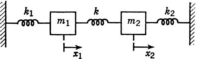
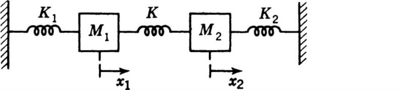
Let us now consider the motion of the system of Fig. 3.1. This system is analogous to the electrical circuit of Fig. 3.2. The state of both of these systems is determined by two quantities. These are the linear displacements of the two masses of the mechanical system (x1,x2) or the mesh charges of the electrical system (q1,q2)- We speak of a system whose motion and position are characterized by two independent quantities as a system having two degrees of freedom. If the position and motion of a system are characterized by n independent quantities, then the system is said to be one of n degrees of freedom.
Fig. 3.1
Fig. 3.2
The equations of motion of the systems of Figs. 3.1 and 3.2 may be obtained by D’Alembert’s principle in the mechanical case or Kirchhoff’s laws for the electrical case. We may pass from one system to the other one by means of the table of analogues of Sec. 2. It is usually simpler to write Kirchhoff’s laws for the system and then translate the electrical quantities to mechanical ones.
Writing Kirchhoff’s law for the fall of potential in the two meshes of the circuit, we have
Translated to mechanical quantities, we have
These equations are linear and homogeneous of the second order of the type discussed in Chap. 2. Their solutions are of the exponential type. To solve them, let us place
where A1, A2, and α may be real or complex. Substituting this into (3.2) and dividing out the factor eαt, we obtain
These are two homogeneous linear equations of the type discussed in Chap. 4. This system of equations has a solution other than the trivial one A1 = A2 = 0 if
Expanding the determinant, we have
This is called the characteristic equation of the system. This equation may be written in the form
It is convenient to introduce the notation
We may then write the characteristic equation in the form
or
We therefore have
The expression under the radical is positive, and the absolute value of the second term is less than that of the first term. Hence α2 is real and negative. Accordingly let us write
Hence
Equation (3.13) gives two values for ω2; let us call them ω1 and ω2. From (3.12) we obtain four values for α:jω1 – jω1, and jω2. We find from our original assumption (3.3) that the solutions for x1 and x2 are of an exponential form, and we obtained four values of α. The general solution may be written in the form
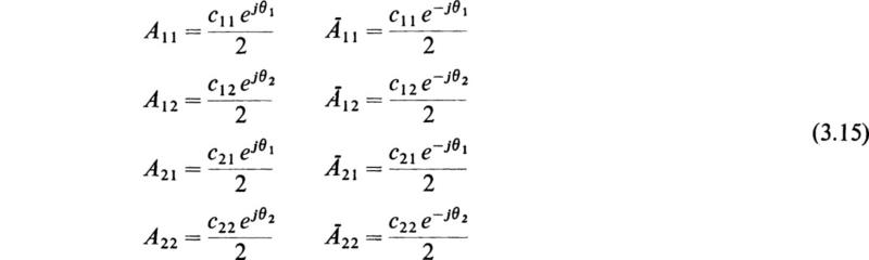
Since x1 and x2 are real, Ā11 must be the conjugate of A11 and similarly for A12 and Ā12, etc. If we write
where c11, c12, c21, c22, θ1 and θ2 are new arbitrary constants, we may then write the solution in the form
The ratios c11/c12 and c12/c22 determined by Eqs.(3.4). Since for each value of α the ratio of the quantities A11/A21 and A12/A22 It appears that in Eqs. (3.16) there are four independent arbitrary constants. We may take them to be c11 cl2, θ1 and θ2. Equations (3.16) show that the most general solution of the system is made up of the superposition of two pure harmonic oscillations. In each of these oscillations the two masses oscillate with the same frequency and in the same phase. The amplitudes of oscillation are in a definite ratio given by Eqs. (3.4).
The pure harmonic oscillations are called the principal oscillations or the principal modes of oscillation of the system.
A very interesting and illuminating special case of the above general theory occurs when the two masses of the system are equal, that is,
and
This is a very symmetric case. Rather than apply the above general theory, it is more convenient to begin with the differential equations of the system. The general equations (3.2) reduce in this case to
If we add the two equations, we have
Let us introduce the new coordinate y1 defined by
We then have
Hence the coordinate y1 performs simple harmonic oscillations of the form
This represents a motion where the two masses swing to the left and right with equal amplitudes in such a manner that the coupling spring is not stressed. If we now subtract the second equation from the first one and let
we obtain
This equation has a solution
Where
This case represents the one in which the two masses move in opposite directions with the same amplitude. We may write the transformation from the x coordinates to the y coordinates in the matrix form
and also
In this very simple case we see that by a linear transformation of the coordinates (x1,x2) to the coordinates (y1, y2) we have effected a separation of the variables so that the motions of the y1 and y2 coordinates are uncoupled. These new coordinates y1 and y2 are called normal coordinates. They will be considered in greater detail in a later section.
The general solution of the system may be written in the form
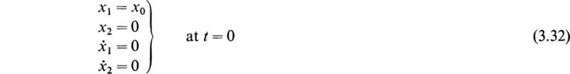
Let us suppose that the motion begins in such a manner that
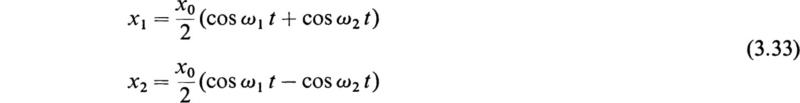
That is, the system is initially at rest, but at t = 0 the mass 1 is displaced a distance x0. In this case the general solution (3.31) reduces to
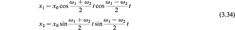
This solution may also be written in the form
If the coupling spring k is weak, then k is small and we may write
where δ is small compared with ω1 and we have approximately
We may then write (3.34) in the form
The motions of the two masses in this case produce a phenomenon called beats. Each mass executes a rapid vibration of angular frequency ω1 with an amplitude that changes slowly with an angular frequency δ. The two masses move in opposite phases so that the amplitude of one reaches its maximum when the other is at rest.
In this section a simple exposition of Lagrange’s equations for conservative systems will be given. For a more complete and detailed treatment the reader is referred to the standard treatises on mechanics.
Let us consider the simple mass-and-spring system of Fig. 4.1. x is a linear coordinate measured from the position of equilibrium of the mass. If the mass is moving with a velocity υ = ![]() , its kinetic energy T is given by
, its kinetic energy T is given by
Fig. 4.1
When the spring is stretched a distance x from its position of equilibrium, then the elastic, or potential, energy stored in the spring is
By Newton’s second law of motion the differential equation governing the motion of the mass is
where ![]() is the acceleration of the mass and F is the restoring force of the spring. The minus sign is introduced because the restoring force F acts in the opposite direction from x, since x is measured from the position of equilibrium. We may also write Eq. (4.3) in the more fundamental form
is the acceleration of the mass and F is the restoring force of the spring. The minus sign is introduced because the restoring force F acts in the opposite direction from x, since x is measured from the position of equilibrium. We may also write Eq. (4.3) in the more fundamental form
If we differentiate the kinetic energy T of (4.1) with respect to v = ![]() , we
, we
obtain
If we differentiate the potential energy V of (4.2) with respect to x, we have
Hence, in terms of the energy functions, the equation of motion may be written in the form
This form of the equation of motion is called Lagrange’s equation of motion and is simply a convenient way of writing Newton’s second law of motion.
Let us now consider the system of Fig. 4.2. This is the system analyzed in Sec. 3. In this case the kinetic energy is given by
Fig. 4.2
The potential energy stored in the springs V is
In this case the kinetic and potential energies are quadratic functions of the linear displacements x1 and x2. In this case, if we form the partial derivative
we obtain the momentum of the first mass. The derivative
is exactly the restoring force acting on the mass M1. We thus see that the first of Eqs. (3.2) may be written in the form
In the same manner the second equation of motion may be written in the form
In this case the motion of the system is given by the two Lagrange equations (4.12) and (4.13).
The importance of Lagrange’s equations is that they hold with respect to any sort of coordinates, not merely the linear coordinates which we have used above. For example, in the symmetric case of Sec. 3 the kinetic and potential energies are given by
We saw that the analysis was vastly simplified by introducing the new coordinates y1 and y2 by the linear transformation
In terms of these new coordinates the kinetic and potential energies become
It was asserted that Lagrange’s equations would hold for the y1, and y2 coordinates. We therefore have
or
and
or
Hence the equations of motion are
and
These were the equations of motion of the symmetric system obtained directly.
In this simple example we see that the introduction of the two new coordinates y1 and y2 reduces the potential- and kinetic-energy expressions to sums of squares. This is a general property of normal coordinates. Each normal coordinate executes simple harmonic oscillations independently of the others.
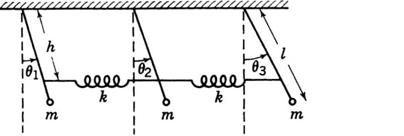
As another example, let us consider the motion of three pendulums of equal masses M and length l connected by springs at a distance h from the suspension points A, B, and C as shown in Fig. 4.3. The masses of the springs and the bars of the pendulums are assumed so small that they can be neglected. The motion of the pendulums may be expressed in terms of the angles θ1 θ2, and θ3 of the pendulums measured from the vertical in a clockwise direction. The kinetic energy of the system is
Fig. 4.3
The potential energy of the system consists of two parts: the energy due to the gravitational force and the strain energy of the springs. If we limit ourselves to a consideration of small oscillations, then θ1 θ2, and θ3 are small quantities. The energy due to gravity is
For small oscillations the springs may be assumed to remain always horizontal. The elongations of the springs are then given by
and
![]()
respectively. The strain energy of the springs is accordingly
The total potential energy of the system is
This mechanical system is analogous to the electrical circuit of Fig. 4.4.
The magnetic energy of the electrical circuit is
Fig. 4.4
where ![]() the mesh currents of the system. The electric energy of the system is
the mesh currents of the system. The electric energy of the system is
These expressions are completely analogous to the kinetic and potential energies of the mechanical system. In this case we have
for the analogous electrical and mechanical quantities. The currents are analogous to the angular velocities of the pendulums. In this case there are three Lagrangian equations of motion of the system:
Performing the differentiation, we obtain
We may find the normal coordinates in this case rather simply. If we add the three equations, we obtain
If we let
Eq. (4.34) becomes
The solution of this equation is
and represents an oscillation of all three pendulums in synchronism with an angular frequency of
If we subtract the last equation (4.33) from the first one and let
We obtain
The solution of the equation
where
If we now add the first and last equations (4.33) and subtract twice the second equation and let
we obtain
This equation has the solution
where
We have thus succeeded in obtaining the three normal coordinates y1, y2, and y3. The three angular frequencies of the system are ω1, ω2, and ω3. If we know the initial displacement and angular velocities of the pendulums, we may determine the six arbitrary constants Ar, Br, r = 1, 2, 3. Then the θr coordinates are given by
These equations are obtained by solving the θr coordinates in terms of the yr coordinates. It may be shown that the kinetic and potential energies (4.25) and (4.28) are reduced to sums of squares in the yr coordinates by this transformation.
In the last section we considered a method of writing the equation of motion of oscillating systems in terms of the expressions for the kinetic and potential energy of the system. We saw that the state of motion of the system could be expressed in terms of different parameters or coordinates.
In this section a proof of Lagrange’s equations will be given for a particle; the proof may be easily generalized to a system of particles and to rigid bodies.
Let us consider a particle of mass M. According to Newton’s second law the equations of free motion of this particle referred to a set of rectangular coordinates are given by
where Fx, Fy, Fz represent the components of the effective force acting on the particle in the x, y, and z directions. Suppose we desire to express these equations of motion in terms of another set of coordinates (q1, q2, q3) related functionally to the rectangular coordinates (x,y,z). We may then express the coordinates (x,y,z) in terms of the coordinates (q1, q2, q3) by
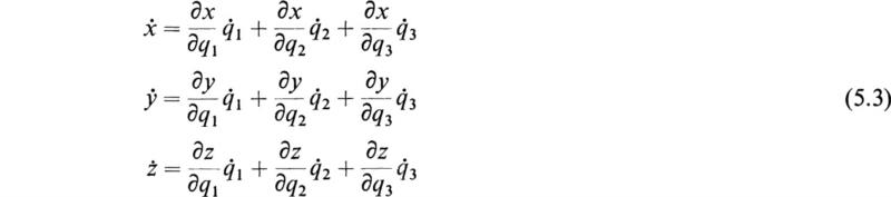
With this notation, on differentiation with respect to time, the expression for the component velocities of the particle ![]() may be put in the form
may be put in the form
where in general ![]() are explicit functions of
are explicit functions of ![]()
Now since
then
Hence
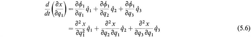
Differentiating the first equation (5.3) with respect to q1 we obtain
If we now compare (5.6) and (5.7) we obtain
with similar relations for y and z.
It is also evident by differentiating the first equation (5.3) with respect to ![]() that
that
with similar relations for y and z.
Let us now assume that we hold the coordinates q2 and q3 fixed and give the coordinate q1 an infinitesimal increment δq1. If δx, δy, and δz are the increments that this produced in x, y, and z, then, if we let δW1 be the work done by the effective forces when the particle undergoes this infinitesimal displacement, we have
as a consequence of Eqs. (5.1). We also have
Hence we may write (5.10) in the form
The rule for the differentiation of a product yields
or
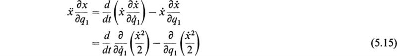
If we substitute the values of δx/δq1 and d/dt(δx/δq1) given by (5.9) and (5.8), we obtain
and similar relations for y and z. However, the kinetic energy of the particle is given by
Hence as a consequence of (5.15) and (5.16) the expression (5.12) may be written in the form
Now, if Q1 δq1 is the work done in the specified displacement of the particle, then it is convenient to regard Q1 as a sort of generalized force. We may write
and we have
By the same reasoning, if q1 and q3 are held constant and q2 is given an increment δq2, we obtain the equation
and in the same manner, holding q1 and q2 constant and giving q3 an increment q3, we obtain
We see that there are as many equations as there are degrees of freedom. The Qr quantities are called generalized forces. The qr quantities are the generalized coordinates.
If there is no loss of energy in the dynamical system under consideration, the generalized forces may be derived from the potential energy of the system V in the form
In this case the free motion of the particle is given by the three Lagrangian equations
By an extension of the above argument it may be shown that in the case of a conservative system having n degrees of freedom its Lagrangian equations are of the form (5.23). In this case there are n generalized coordinates (q1, q2, . . . ,qn) and there are n equations.
We notice that in the simple examples of Lagrange’s equations discussed in Sec. 4 we had
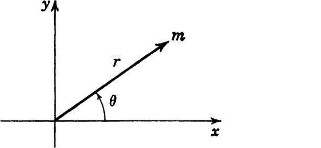
The reason for this was that the kinetic energy in the systems discussed in that section was not a function of the coordinates, but only of the velocities of the system. As an example of a system where the kinetic energy is a function of the generalized coordinates qr as well as the generalized velocities qr, consider the two-dimensional motion of a particle in the xy plane as shown in Fig. 5.1.
In this case we have
Let us assume that the particle is attracted to the origin by a force proportional to the distance so that the particle has a radial force Fr directed toward the origin given by
In this case the potential energy is given by
To describe the motion of the particle it is convenient to use the polar coordinates r and θ as the generalized coordinates. These coordinates are related to the cartesian coordinates x and y by the equations
In terms of these coordinates the kinetic energy becomes
Fig. 5.1
The Lagrangian equations of motion are
or
and
or
Equations (5.31) and (5.33) are the equations of motion of the system. Equation (5.33) expresses the conservation of angular momentum of the system. The term is ∂T/∂r is seen to give rise to the centrifugal-force term. Terms of the form dT/∂r, which are absent in rectangular coordinates, may be regarded as a sort of fictitious force introduced by using generalized coordinates.
A very important class of problems in the theory of vibrations is that in which a dynamical system is performing free or forced oscillations without friction. The determination of the natural frequencies and modes of oscillations of the torsional vibrations of an engine, the oscillations of spring-mounted machinery, the oscillations of electrical networks whose resistance is so small as to be neglected, etc., are problems that fall in this category.
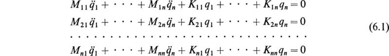
The Lagrangian equations of motion of a general conservative system of n degrees of freedom oscillating in the neighborhood of a position of equilibrium may be written in the form
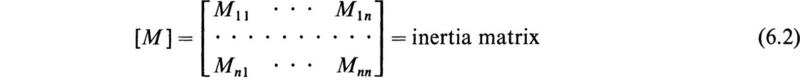
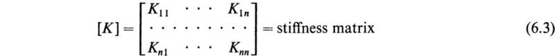
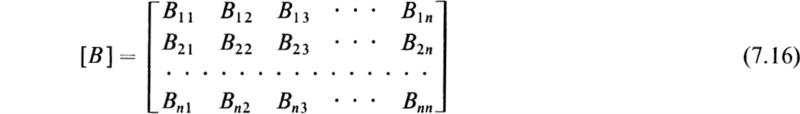
where (q1, . . . , qn) are generalized coordinates, Mrs are inertia coefficients, and Krs are stiffness coefficients. These are the equations governing the motion of the most general conservative system performing free oscillations in the neighborhood of a position of equilibrium. The examples discussed in Secs. 3 and 4 are special cases of this general system. The analysis of these equation is greatly facilated by writing them in matrix notation. If we let
the set of Eqs. (6.1) may then be written in the convenient form
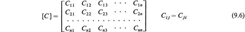
The coefficients Mrs and Krs have the important property that
Hence the matrices [M] and [K] are symmetric. The kinetic and potential energies of the system may be written in the convenient matrix form
where ![]() and {q}' are the transposed matrices of the column matrices
and {q}' are the transposed matrices of the column matrices ![]() and {q} and are hence row matrices. This is the notation used in Chap. 4.
and {q} and are hence row matrices. This is the notation used in Chap. 4.
Let us consider solutions of Eq. (6.5) corresponding to pure harmonic motion of the form
where {A} is a column matrix of amplitude constants, ω is the angular frequency of the oscillation, and θ is an arbitrary phase angle. Substituting this into Eq. (6.5), we obtain
This represents a set of homogeneous algebraic equations in the arbitrary amplitude constants {A}.
It is convenient to premultiply both sides of Eq. (6.9) by [K]-1 the inverse of K. We then obtain
where I is the unit matrix of the nth order. The matrix [K]-1[M] is usually called the dynamical matrix. That is, we have
In terms of the dynamical matrix the set of Eq. (6.10) may be written in the form
If we now write
then (6.12) may be written in the form
This set of equations will have solutions other than the trivial one of zero if the determinant of the system vanishes. That is,
This is an equation of the nth degree in Z. It may be proved that all the roots are real and positive. Ordinarily this equation will have n distinct roots Z1, Z2, Z3, . . . , Zn. To each root Zr there corresponds a value ωr of ω, given by
These are the natural angular frequencies of the system. We thus see that our original assumed solution (6.8) has led us to n values of n. Each value ωr of ω gives a solution of the form
Since the original set of equations is linear, we may write the general solution by summing solutions of the form (6.17). We then have the general solution
The column matrices {A(r)} are called the modal columns. Every oscillation represented by each modal column is called a principal mode of oscillation of the system. The number of principal oscillations is equal to the number of degrees of freedom of the system.
Every principal oscillation is a pure harmonic motion. The most general form of oscillation of a system of n degrees of freedom consists of the superposition of n pure harmonic motions. The frequencies of the principal oscillations are called the natural frequencies of the system. The lowest frequency is called the fundamental frequency.
The modal columns satisfy Eq. (6.9) with the proper value of ω. For example, the rth modal column satisfies the equation
This equation fixes the ratios of the numbers of the rth modal column. If, for example, the first number A1(r) is chosen arbitrarily, then by Eq. (6.19) the numbers A2(r) A3(r), . . . , An(r) may be expressed in terms of A1(r) We thus see that the general solution (6.18) contains only 2n arbitrary constants, since any number in any modal column may be specified arbitrarily and the phase angles θr are arbitrary.
The modal columns possess a very interesting and important property that will now be derived. Let us write the equation satisfied by the mode {A(s)}. This equation is
Let us premultiply Eq. (6.19) by {A(s)}’ and Eq. (6.20) by {A(r)}′. We then obtain
Now, by a fundamental theorem of matrix algebra, if we have the product of three conformable matrices [a][b][c], then the transpose of the product is given by
(see Chap. 3). If we then take the transpose of Eq. (6.21) and use the reversal law of transposed products (6.23), we obtain
in view of the fact that the matrices [M] and [K] are symmetric, and hence [M] ′ = [M] and [K]′ = [K].
If we now subtract Eq. (6.24) from Eq. (6.22), we obtain
Now, by hypothesis, ωs and ωr are two different natural frequencies of the system; hence ωs ≠ ωr. It follows that
This relation is known as the orthogonality relation for the principal modes of oscillation.
A very useful and important method for the determination of the roots of the frequency equation (6.15) and the determination of the normal modes of a conservative system has been presented by W. J. Duncan and A. R. Collar.† This method is most convenient in that it avoids the expansion of the determinantal equation (6.15) and the solution of the resulting high-degree equation. The modal columns {A(r)} are also most simply obtained. Because of its great utility and increasing usefulness a brief treatment of the method will be given in this section.
We see from Eq. (6.14) that the rth modal column satisfies the equation
where Zr is the rth root of the frequency or determinantal equation (6.15). [U] is the dynamical matrix of the system. If we premultiply Eq. (7.1) by U, we obtain
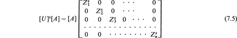
If we premultiply (7.1) by [U] s time, we obtain
We have n equations of this type, one for each modal column {A(r)} and its associated root Zr. Let us now construct a square matrix [A] from the various modal columns {A(r)} in the following manner:
The set of Eqs. (7.3) may be conveniently written in the form
Postmultiplying (7.5) by [A]–1 we obtain
Now let the roots Zr of the determinantal equation be arranged in descending order of magnitude; that is, let Z1 be the largest root of the determinantal equation, Z2 the next largest, etc., or
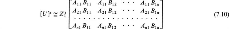
assuming that the roots are all distinct. Now let us assume that s in Eq. (7.6) is so great that
If this is true, then only the terms corresponding to the dominant root Z1 need be retained. By direct multiplication we have for s sufficiently large
As a consequence of this property of the dynamical matrix [U] we may perform the following procedure, which will yield the dominant root Z1 of the system as well as the modal column associated with this root.
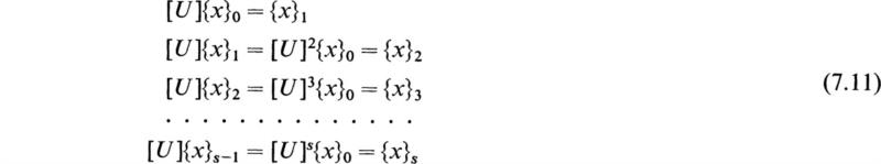
Let us select an arbitrary column matrix {x}0 and form the following sequence:
In view of Eq. (7.10) we have or a sufficiently large s
where
That is, by repeated multiplication of the column matrix {x}0 by the dynamical matrix [U], we eventually reach a stage where further multiplication by [U] merely multiplies every element of the column matrix {x}s–1 by a common factor. This common factor is Z19 the dominant root of the determinantal equation. By (6.16) the fundamental angular frequency ω1 is given by
We also see that the elements of the column matrix {x}s are proportional to those of the modal matrix {A(1)}.
We now turn to a procedure by which we may obtain the next largest root Z2 and its appropriate mode. To do this, let us place s = 1 in Eq. (7.6) and premultiply both sides by [A]-1. We then obtain, since [A]-1 = [B],
The matrix B is given by
We thus see that if we take a typical row [Br] of the square matrix [B] in the form
then as a consequence of Eq. (7.15) we have
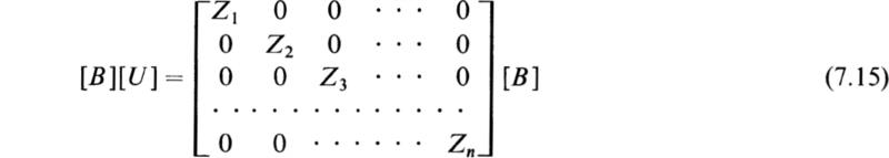
We also have, by (7.1), the relation
a relation satisfied by the modal column {A(r)}. Now since the dynamical matrix [U] is equal to [K]–1[M], we may write (7.19) in the form
If we premultiply both sides of this equation by M, take the transpose of both sides, and use the reversal law of transposed products, we obtain
Comparing Eqs. (7.21) and (7.18), we see that they are identical in form; hence we have
where ar is a proportionality factor. Equation (7.22) is of great importance in determining the higher roots of the determinantal equation as well as the modal columns corresponding to these roots.
We notice that since [B] = [A]–1 we have
where I is the unit matrix of the nth order. Hence the row matrices [Br] and the modal column matrices {A(r)} have the property that
The general solution of the problem under consideration is given in terms of the natural angular frequencies ωr and the modal columns {A(r)} in the form
where the θr are the arbitrary phase angles determined from the initial conditions of the system at t = 0. The Cr are arbitrary constants also determined from the initial conditions of the system.
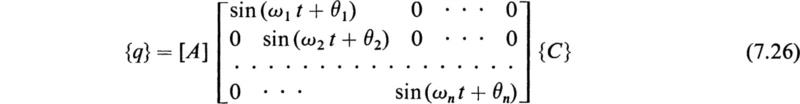
This equation may also be written in the convenient matrix form
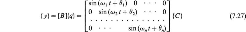
If we premultiply both sides of (7.26) by [B] = [A]-l, we obtain
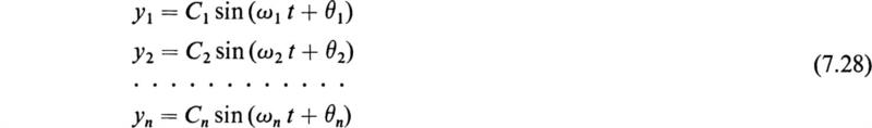
Hence we have
The yr quantities are the normal coordinates of the system.
By Eq. (7.12) we have seen how the fundamental frequency ω1 and the fundamental mode {A(1)} may be obtained. We shall now develop a procedure by which the higher angular frequencies and the corresponding modal columns may be obtained
If we premultiply (7.25) by the row matrix [B1], we have in view of (7.24)
If now the fundamental mode is absent, we have
Hence, expanding this equation, we obtain
or
This set of equations may be written in the matrix form
Or if we call the square matrix above [S], we have
This constrains the coordinates in such a manner that the fundamental mode is absent. The original differential equations of the system (6.5) may be written in terms of the dynamical matrix in the form
where I is the unit matrix of the nth order. If we now differentiate Eq. (7.34) twice with respect to time, we have
Substituting this into (7.35), we obtain
If we let
Eq. (7.37) becomes
This set of equations has the same form as the original set (7.35). It represents a system whose dynamical matrix is [U]1 and whose natural frequencies and modes are the same as those of the original system, but since we have used the constraint (7.34), the fundamental frequency and mode are now absent.
By carrying out the same procedure with the matrix [U]1 that was performed with the matrix [U], we obtain the root Z2 and hence the next higher natural frequency ω2 together with the corresponding mode. We then obtain a new row matrix [B2] by Eq. (7.22) and repeat the procedure until all the angular frequencies and all the modal columns of the system have been found. An example of the general procedure will now be given.
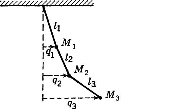
As a simple numerical example of the above theory, let us consider the oscillations of a triple pendulum under gravity in a vertical plane. This example is given by Duncan and Collar in their fundamental paper referred to in Sec. 7. The dynamical system under consideration is given by Fig. 8.1.
We shall consider the case of small oscillations, and for the coordinates of the system we shall take the small horizontal displacements of the masses M1, M2, M3, respectively, from the equilibrium position. The first step in the procedure is to compute the dynamical matrix [U].
Fig. 8.1
If we apply a set of static forces F1, F2, F3 in the direction of the coordinates q1 q2, and q3, we may write the relation between the displacements q1, q2, and q3 and the forces F1, F2, F3 in the form
where the square matrix [K] is the stiffness matrix. We may premultiply by [K]-1 and obtain the displacements in terms of the forces in the form
where the matrix [ø] = [K]-1 the flexibility matrix. Since Krs = Ksr, we have
That is, the flexibility matrix is a symmetric matrix.
In terms of the flexibility matrix the dynamical matrix is given by
To determine the elements of the flexibility matrix, it is necessary only to impose a unit force F1 on the system and compute or measure the corresponding deflections (q1q2q3). This gives the elements of the first column of [ø]. Applying a unit force F2 and obtaining the corresponding deflections yields the second column of [ø], etc.
If a static unit force is applied horizontally to mass M1 then the three masses will each be displaced a distance a given by
Hence the first column of the flexibility matrix is given by
When a unit force is applied horizontally to M2, M1 will again be displaced a distance a, but M2 and M3 will each be displaced a distance a + b, where
Hence the second column of the matrix [ø] is given by
Applying a unit horizontal force to M3 displaces M1 a distance a; M2 a distance a + b; and M3 a distance a + b + c, where
The third column of the flexibility matrix is
Hence the flexibility matrix is given by
The mass matrix, in this case, has the diagonal form
Hence the dynamical matrix is given by
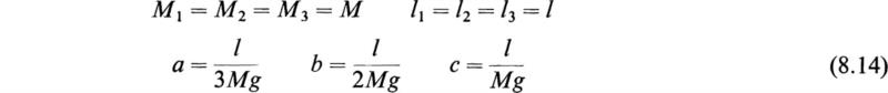
As a numerical example, let us take the case where all the masses are equal and the lengths of the pendulums are equal. In this case we have
Hence the dynamical matrix in this case becomes
Equation (6.12) reduces in this case to
If we let
then Eq. (6.14) becomes
where [u] is the numerical part of the dynamical matrix [U], and the factor 6g/l has been absorbed into ![]() .
.
The angular frequencies are given by
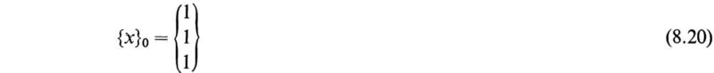
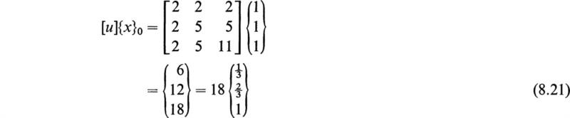
To find the roots Zr, we begin the iterative procedure of Eq. (7.11). If we choose for our arbitrary column {x}0 the column
we begin the sequence
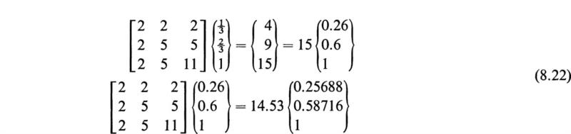
It is unnecessary to carry the common factor 18 in the further operations since it is the ratios of the successive elements in the multiplications that are important. Dropping the factor 18 and continuing, we have
After nine multiplications we have
Repeating the process merely multiplies the column matrix by the factor 14.4309; we therefore have
The fundamental frequency of the oscillation is given by
The modal column {A(1)} is proportional to the column

To obtain the higher harmonics, we first make use of Eq. (7.22) to obtain the row B1. In this case we have
Since a1 is an arbitrary factor and we are interested only in a row proportional to [B1] we may take B1 equal to [B1]. We may take B1 equal to [0.254885, 0.584225, 1] The matrix [S] of (7.34) is now given by
We then obtain
This is the dynamical matrix that has the fundamental mode absent. We now repeat the iterative procedure by again choosing an arbitrary column matrix {x}0; we thus find
After 15 multiplications the column repeats itself, and the multiple factor is
The modal column {A(2)} for this approximation may be taken to be
Hence the first overtone has this mode and a frequency given by
Again by Eq. (7.22) we may take the row {B2} equal to {A(2)}′.
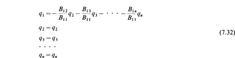
The condition for the absence of the second overtone is
Solving this for q1 we have
We may eliminate q1 between this equation and the equation
We thus obtain
This ensures that both the fundamental and first-overtone modes are absent from the oscillation. Equation (8.36) may be written in the convenient matrix form
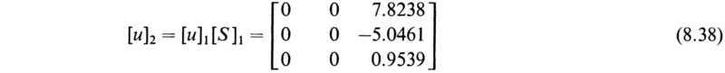
We now construct a new dynamical matrix [u]2 that has the fundamental and overtone modes absent; this new matrix is given by
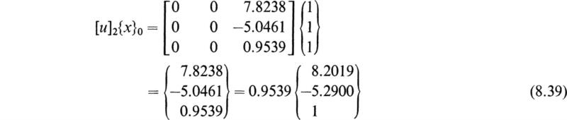
We again repeat the iterative process and obtain
Repeating the process merely repeats the factor 0.9539; so it is unnecessary to go further. We thus have
The highest frequency is given by
The mode {A(3)} corresponding to this frequency may be taken to be
to a factor of proportionality. The modal matrix may be taken to be
In this case, because of the simplicity of the mass matrix [M], we may take
the transpose of matrix [A].
The normal coordinates are then given by
In the last few sections the general theory of conservative systems has been considered. These systems are characterized completely by their kinetic-and potential-energy functions and are of great practical importance. In many problems that arise in practice the frictional forces are relatively small and may be disregarded and the system treated as a conservative one.
The mathematical analyses of vibrating systems that contain frictional forces of a general nature usually lead to a formulation involving nonlinear differential equations (see Chap. 15). However, in a great many practical problems, the frictional forces involved are proportional to the velocities of the moving parts of the system. Frictional forces of this type are present in systems that contain viscous friction. The mathematical solution of vibration problems of systems involving viscous friction leads usually to the solution of sets of linear equations and is relatively simple.
The Lagrangian equations of Sec. 4 can be generalized to take into account viscous friction. In order to do this, it is necessary to compute the rate at which energy is dissipated by the viscous frictional forces. This may be done by considering a single particle moving along the x axis undergoing damping so that the resisting frictional force impeding its motion is
The work done by the frictional force during a small displacement ![]() and the amount of energy δW dissipated is
and the amount of energy δW dissipated is
The time rate at which energy is dissipated in this case is δW/δt = c![]() 2. Let the function F be defined by the equation
2. Let the function F be defined by the equation
This function is called the dissipation function and represents half the rate at which the energy of the particle is dissipated by the viscous frictional force. The frictional force fr may therefore be obtained by the following equation:
By an extension of the above analysis to the case of a system having n degrees of freedom undergoing viscous friction, it can be shown that the dissipation function of the entire system in general has the form
where ![]() are the generalized velocities of the system and the coefficients C11, C12, C22, ... in general depend on the configuration of the system, though for the case of small vibrations in the neighborhood of a configuration of stable equilibrium these coefficients can be treated with good accuracy as being constant. In such cases it is convenient to introduce the damping matrix
are the generalized velocities of the system and the coefficients C11, C12, C22, ... in general depend on the configuration of the system, though for the case of small vibrations in the neighborhood of a configuration of stable equilibrium these coefficients can be treated with good accuracy as being constant. In such cases it is convenient to introduce the damping matrix
The elements of the damping matrix [C] are the viscous-friction damping coefficients Cij. The matrix [C] is a symmetric matrix. In terms of this matrix the dissipation function F may be written in the following concise form,
where ![]() is the transpose of the generalized velocity matrix (q).
is the transpose of the generalized velocity matrix (q).
The dissipation function F represents half the rate at which energy is being dissipated from the entire system as it moves under the influence of viscous friction. The generalized forces fi that arise from the viscous friction of the system are
The Lagrangian equations of the system then take the form
The left-hand member of (9.9) represents the effect of the inertia terms of the system; the terms of the right-hand member are the various generalized forces of the system. (1) The term –(∂V/∂qi) takes into account forces that may be derived from a potential function V such as gravitational forces, forces due to the presence of elastic springs, etc. (2) The term ![]() takes into account the effect of retarding forces due to viscous friction. (3) The term Qi includes all other forces acting on the system, such as time-dependent disturbing forces.
takes into account the effect of retarding forces due to viscous friction. (3) The term Qi includes all other forces acting on the system, such as time-dependent disturbing forces.
In terms of the inertia matrix [M], the stiffness matrix [K], and the damping matrix [C] of the system the Lagrangian equations (9.9) may be written in the following concise form:
The elements of the column matrix (Q) are the generalized forces Qi of the system.
The electrical networks of Chap. 5 may be regarded as special dynamical systems that are characterized by the following functions:
In these expressions the ![]() are the various mesh currents of the circuit, the elements of {q} are the various mesh charges of the circuit, and the square matrices [L], [S], and [R] are the inductance, elastance, and resistance matrices of the circuit. In this case T represents the magnetic energy of the system, V the electric energy of the system, and F is one-half the power dissipated by the resistances of the circuit. The Lagrangian equations (9.9) now take the following form:
are the various mesh currents of the circuit, the elements of {q} are the various mesh charges of the circuit, and the square matrices [L], [S], and [R] are the inductance, elastance, and resistance matrices of the circuit. In this case T represents the magnetic energy of the system, V the electric energy of the system, and F is one-half the power dissipated by the resistances of the circuit. The Lagrangian equations (9.9) now take the following form:
The elements of the column matrix {E} are the various mesh potentials of the electrical circuit.
If the generalized forces Qi driving the nonconservative system are all equal to zero, then the set of Eqs. (9.10) reduce to
This set of differential equations determines the nature of the free oscillations of the system. In order to solve this set of equations, assume a solution of the exponential form
where m is a number to be determined and {A} is a column of constants. If this assumed form of solution is substituted into (9.13), the following result is obtained:
If (9.15) is divided by the scalar factor emt, a set of linear homogeneous equations in the column of constants {A} is obtained. For this set of equations to have a nontrivial solution, it is necessary that the determinant of the coefficients must vanish; hence we must have
This equation is called Lagrange’s determinantal equation for m. In general it is of degree 2n. The following properties concerning the roots of Δ(m) may be proved :†
1. None of the roots is real and positive.
2. If [C] = [0], there is no dissipation of energy and the system is a conservative one. In this case the roots are all pure imaginaries.
3. If [M] = [0] or [K] = [0] so that the system is devoid of inertia or of stiffness and [C] ≠ [0], the roots are real and negative so that the motion dies away exponentially.
4. If the elements of the damping matrix [C] are not too large, all the roots are conjugate complex numbers with a negative real part. This is the most frequent case in practice.
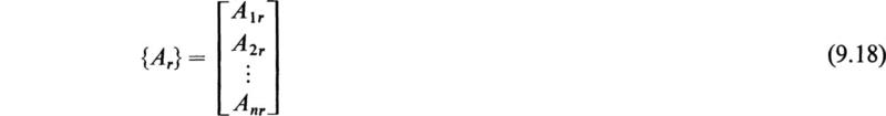
Let it be supposed that Eq. (9.16) has 2n distinct roots (m1,m2,m3, . . . , m2n). Then as a consequence of (9.15) there are 2n equations of the following type:
where {Ar} represents a column of constants associated with the root mr. Each column {Ar} has the form
Equation (9.5) fixes the ratios
The theory of linear differential equations indicates that to obtain a general solution of the set of Eqs. (9.13) we must take the sum of the particular solutions ![]() for all the roots mr. We thus obtain the following general solution:
for all the roots mr. We thus obtain the following general solution:
It must be noted that the ratios of the A’s in any one column are determined by the linear equations (9.17); therefore there is still a factor that is arbitrary for each column and hence 2n in all. Thus the general solution (9.20) contains 2n arbitrary constants, as it should.
If the roots of (9.16) are complex, they occur in conjugate complex pairs of the form
In this case the general solution (9.20) contains terms of the following type:
where {Br} represents a column of constants and the θr are phase angles. In this case the general solution of (9.13) takes the form
It may easily be shown that the {Br} columns satisfy (9.17) in the same manner as do the {Ar} columns, and hence the ratios of the B’s in each column are fixed. Each column then contains an arbitrary constant in the phase angle θr belonging to the column. The following results may be stated:
If the roots of the determinantal equation (9.16) are distinct and conjugate complex quantities, then the motion of a dynamical system having n degrees of freedom slightly displaced from a position of stable equilibrium may be described as follows:
Each coordinate performs the resultant of n damped harmonic oscillations of different periods. The phase and damping factors of any simple oscillation of a particular period are the same for all the coordinates. The absolute value of the amplitude of any particular coordinate is arbitrary, but the ratios of the amplitudes for a particular period for the different coordinates are determined solely by the nature of the system. The 2n arbitrary constants determine the n amplitudes and phases of the system. These arbitrary constants are found from the values of the n coordinates {q} and the n velocities ![]() for a particular instant of time.
for a particular instant of time.
The classical method of solution for the general nonconservative system consists in obtaining the determinantal equation (9.16), expanding the determinantal equation, then solving it for the 2n roots (m1,m2,m3, . . . ,m2n) by the Graeffe method of Appendix D. Once the roots mr of the determinantal equation have been found, the ratios of the columns (Br) can be calculated by the use of (9.17). Finally the arbitrary constants are determined from a knowledge of the initial conditions of the system.
In a fundamental paper by Duncan and Collar† an iterative method similar to that discussed in Sec. 7 for the determination of the modes, decrement factors ar and frequencies ωr of nonconservative systems is given. The basic principle that underlies the method is to write the system of differential equations (9.13) as a first-order system by the introduction of the following partitioned matrix:
The column matrix {y} thus contains 2n elements, the n coordinates (q), and the n velocities ![]() . If the following square partitioned matrix of the 2nth order is introduced,
. If the following square partitioned matrix of the 2nth order is introduced,
where [0] is the nth-order zero matrix and [I] is the nth-order unit matrix, then the system of differential equations (9.13) may be written in the following form:
In order to solve the first-order system of differential equation (10.3), assume a solution of the form
If the assumed solution (10.4) is substituted into the differential equation (10.3), the following result is obtained:
If the scalar factor emt is divided out of Eq. (10.5), the result may be written in the form
where I is the unit matrix of order 2n. The matrix
is the characteristic matrix of the matrix [υ]. The characteristic equation of [υ] is
The roots m1, m2, m3, . . . , m2n are the eigenvalues of the matrix [v]9 and the columns {A J, {A2}, {A^}, . . . , {A2n} satisfy equations of the form
The columns {Ar} are therefore the eigenvectors of the matrix [υ].
The root mr, having the largest modulus, may be determined by setting up a sequence similar to that of (7.11) of the form
where {x}0 is an arbitrary column matrix of the 2nth order. It will be found that for a sufficiently large s continued multiplications give rise merely to multiplicative factors. These factors enable the eigenvalue having the largest modulus to be determined, and also the associated eigenvector can be found. The details of the practical numerical procedure are somewhat lengthy and will be found in the above paper and in the book by Frazer, Duncan, and Collar (1938).
Let us suppose that on each coordinate of the general nonconservative system there is impressed a harmonically varying force
In this case the differential equations (9.13) become
where {F} is a column matrix whose elements are the amplitudes of the impressed forces Fr. We replace cosωt by Reejωt and solve the equation
retaining only the real part of the particular solution. To do this, let us assume
where {Q} is a column of amplitude constants to be determined. Substituting this assumed solution into (11.4) and dividing by the common factor ejωt, we have
If we let
then on premultiplying both sides of (11.6) by [Z]-1 = [Y], we have
The steady-state solution of the forced oscillation is now given by
where Re signifies “the real part of.” The matrix [Z] is sometimes termed in the literature the mechanical impedance matrix and [Y] the mechanical admittance matrix. Equation (11.8) represents the forced oscillations after the damped free oscillations have vanished.
It must be noted that, if [R] = [0] and the system is conservative, then, if co happens to coincide with one of the natural frequencies of the system, [Z] as given by Eq. (11.6) vanishes and we have the case of resonance.
1. Obtain the flexibility matrix of the three-pendulum system of Fig. 4.3. Write the dynamical matrix of the system.
2. An electric train is made up of three units: a locomotive and two passenger cars. Each unit has a mass M, and the spring constants of the coupling connecting them are equal to K. Write the Lagrangian equation of motion of the system. Draw the equivalent electrical circuit, and determine the natural frequencies of the system.
3. If in the system of Prob. 2 identical shock absorbers that act by viscous friction are placed between the three units, determine the smallest value of the damping factor R so that the relative motion of the locomotive and cars is not oscillatory.
4. A long train of n identical units of mass M coupled by springs of spring constants all equal to K is oscillating. Draw the equivalent electrical circuit, and write the frequency equation of the system.
5. A uniform shaft free to rotate in bearings carries five equidistant disks. The moments of inertia of four disks are equal to J, while the moment of inertia of one of the end disks is equal to 2J. Set up the dynamical matrix, and obtain the lowest natural frequency by the iterative matrix method of Sec. 7. Draw the equivalent electrical circuit.
6. A particle of mass M is attracted to a center by a force proportional to the distance, or Fz = –ax, Fy = –ay. Write the equations of motion of the particle. Show that x and y execute independent simple harmonic vibrations of the same frequency.
7. Solve Prob. 6 by using polar coordinates.
8. Two balls, each of mass M, and three weightless springs, one of length 2d and the others of length d, are connected together in the arrangement spring d—ball—spring 2d— ball—spring d, and the whole device is stretched in a straight line between two points, with a given tension in the spring. Gravity is neglected.
Investigate the small vibrations of the balls at right angles to the straight line, assuming motion only in one plane. Set up the equations of motion. Determine the natural frequencies and the normal modes. What are the normal coordinates?
9. One simple pendulum is hung from another; that is, the string of the lower pendulum is tied to the bob of the upper one. Discuss the small oscillations of the resulting system, assuming arbitrary lengths and masses. Determine the natural frequencies and obtain the normal coordinates in the case of equal masses and equal lengths of strings.
10. Consider the case of the three coupled pendulums of Fig. 4.3. In this case assume that each pendulum is retarded by a viscous force proportional to its angular velocity. Consider an equal retarding force on each pendulum. Draw the equivalent electrical circuit, and obtain the general solution of the equations of motion. Assume that the damping is so small that oscillations are possible.
11. A particle subject to a linear restoring force and a viscous damping is acted on by a periodic force whose frequency differs from the natural frequency of the system by a small quantity.
The particle starts from rest at t = 0 and builds up the motion. Discuss the whole problem, including initial conditions. Consider what happens when the frequency gets nearer and nearer the natural frequency and the damping gets smaller and smaller.
12. Show that for a particle subject to a linear restoring force and viscous damping the maximum amplitude occurs when the applied frequency is less than the natural frequency. Find this resonance frequency. Show that maximum energy is attained when the applied frequency is equal to the natural frequency.
13. Two small metal spheres A and B of equal mass m are suspended from two points A' and B' at a distance a apart on the same horizontal line by insulating threads of equal length s. They are then charged with equal charges +q. If A is pulled aside a short distance s1 and B a short distance s2 (both small in comparison with a) in the plane formed by the equilibrium position of both threads, determine the resulting motion in this plane. Determine the frequencies of oscillation of the system.
14. Two particles of mass m connected by a weightless spring of unstressed length s and spring constant k are set moving in an arbitrary manner on a smooth horizontal plane. Set up and solve Lagrange’s equations for this case.
15. Discuss the oscillations of the coupled triple pendulum of Sec. 4 by the matrix-iteration method of Sec. 7. Determine the lowest and highest frequencies of oscillating by matrix iteration assuming that Mgl/kh2 = 1.
1905. Routh, E. J.: “Advanced Rigid Dynamics,” The Macmillan Company, New York.
1926. Maxfield, J. P., and H. C. Harrison: Methods of High Quality Recording and Reproducing of Music and Speech Based on Telephone Research, Bell System Technical Journal, vol. 5, pp. 493–523, July.
1937 Timoshenko, S.: “Vibration Problems in Engineering,” D. Van Nostrand Company, Inc., Princeton, N.J.
1938 Frazer, R. A., W. J. Duncan, and A. R. Collar: “Elementary Matrices and Some Applications to Dynamics and Differential Equations,” Cambridge University Press, New York.
1940. Den Hartog, J. P.: “Mechanical Vibrations,” 3d ed., McGraw-Hill Book Company, New York.
1940. Kármán, T. V., and M. A. Biot: “Mathematical Methods in Engineering,” McGraw-Hill Book Company, New York.
1943. Olson, H. F.: “Dynamical Analogies,” D. Van Nostrand Company, Inc., Princeton, N.J.
1948. Brown, G. S., and D. P. Campbell: “Principles of Servomechanisms,” John Wiley & Sons, Inc., New York.
1948. Mason, W. P.: “Electromechanical Transducers and Wave Filters,” D. Van Nostrand Company, Inc., Princeton, N.J.
1948. Timoshenko, S. P., and D. H. Young: “Advanced Dynamics,” McGraw-Hill Book Company, New York.
1951. Goldstein, H.: “Classical Mechanics,” Addison-Wesley Publishing Company, Inc., Reading, Mass.
1951. Scanlan, R. H., and R. Rosenbaum: “Aircraft Vibration and Flutter,” The Macmillan Company, New York.
1957. Morrill, B.: “Mechanical Vibrations,” The Ronald Press Company, New York.
1963. Paskusz, G. F., and B. Bussel: “Linear Circuit Analysis,” Prentice-Hall, Inc., Englewood Cliffs, N.J.
1963. Pipes, L. A.: “Matrix Methods for Engineering,” Prentice-Hall, Inc., Englewood Cliffs, N.J.
1965. Thomson, W. T.: “Vibration Theory and Applications,” Prentice-Hall, Inc., Englewood Cliffs, N.J.
† W. J. Duncan and A. R. Collar, A Method for the Solution of Oscillation Problems by Matrices, Philosophical Magazine, ser. 7, vol. 17, p. 865, 1934.
† See A. G. Webster, “The Dynamics of Particles and of Rigid Bodies,” Teubner Verlagsgesellschaft, Leipzig, 1925.
† W. J. Duncan and A. R. Collar, Matrices Applied to the Motions of Damped Systems, Philosophical Magazine, ser. 7, vol. 19, p. 197, 1935.