In the theory of operational calculus a mathematical technique that has proved to be a powerful method for solving differential equations and general system analysis is the Laplace transform. Before we proceed to a detailed exposition of the theory of Laplace transforms, it is of some interest to list some of the better-known uses of the Laplace-transform theory in applied mathematics.
1. The solution of ordinary differential equations with constant coefficients: The Laplace transform is of use in solving linear differential equations with constant coefficients. By its use the differential equation is transformed into an algebraic equation which is readily solved. The solution of the original differential equation is then reduced to the calculation of inverse transforms usually involving the ratio of two polynomials. The inverse transforms required may be obtained by consulting a table of Laplace transforms or by evaluating the inverse integral by the calculus of residues.
The Laplace-transform method is particularly well adapted to the solution of differential equations whose boundary conditions are specified at one point. The solution of differential equations involving functions of an impulsive type may be solved by the use of the Laplace transform in a very efficient manner. Typical fields of application are the following:
a. Transient and steady-state analysis of electrical circuits [4, 7–9, 11, 15, 16]. †
b. Applications to dynamical problems (impact, mechanical vibrations, acoustics, etc.) [5–8, 10, 17].
c. Applications to structural problems (deflection of beams, columns, determination of Green’s functions and influence functions) [6–10, 13].
2. The solution of linear differential equations with variable coefficients: By the use of the Laplace-transform theory a linear differential equation whose coefficients are polynomials in the independent variable t is transformed into a differential equation whose coefficients are polynomials in the transform variables. In many cases the transformed equation is simpler than the original, and it can be readily solved. The inverse transform of the solution of this equation gives the solution of the original equation [17, 18]. Van der Pol [11, 18] has shown how this may be done in the case of Bessel functions and Legendre and Laguerre polynomials.
3. The solution of linear partial differential equations with constant coefficients: One of the most important uses of the Laplace-transform theory is its use in the solution of linear partial differential equations with constant coefficients that have two or more independent variables. The procedure employed is to take the Laplace transform with respect to one of the independent variables and thus reduce the partial differential equation to an ordinary one or one having a smaller number of independent variables. The transformed equation is then solved subject to the boundary conditions involved, and the inverse transform of this solution gives the required result. Problems involving impulsive forces and wave propagation are particularly well adapted for solution by the Laplace-transform method. In many cases it is possible to express the operational solution of the partial differential equation involved in a series of exponential terms and then interpret the solution as a succession of traveling waves. Typical physical problems that may be solved by the procedure outlined above are the following:
a. Transients and steady-state analysis of heat conduction in solids [5, 6, 13, 16, 17].
b. Vibrations of continuous mechanical systems [6–8, 13, 17].
c. Hydrodynamics and fluid flow [6–8, 19].
d. Transient analysis of electrical transmission lines and also of cables [4, 6, 11, 13, 15, 16].
e. Transient analysis of electrodynamic fields [5, 7].
f. Transient analysis of acoustical systems [7, 8].
g. Analysis of static deflections of continuous systems (strings, beams, plates) [6, 9, 17].
4. The solution of linear difference and difference-differential equations: The Laplace-transform theory is very useful in effecting the solution of linear difference or mixed linear-difference–differential equations with constant coefficients. Difference equations arise in systems where the variables change by finite amounts. Typical fields of application of difference equations are the following:
a. Electrical applications of difference equations [6, 9, 11, 13] (artificial lines, wave filters, network representation of transformer and machine windings, multistage amplifiers, surge generators, suspension insulators, cyclic switching operations).
b. Mechanical applications of difference equations [6, 7, 9, 17].
c. Applications to economics and finance [9] (annuities, mortgages, interest, amortization, growth of populations).
d. Systems with hereditary characteristics [20] (retarded control systems, servomechanisms).
5. The solution of integral equations of the convolution, or Faltung, type: Equations in which the unknown function occurs inside an integral or integral equations are encountered quite frequently in applied mathematics. If the integral equation happens to be of the convolution, or Faltung, type, the use of the Laplace-transformation theory transforms the equation into an algebraic equation in the transform variable and it is readily solved. Typical problems leading to this type of equation are the following:
a. Mechanical problems such as the tautochrone [14, 17].
b. Economic problems (mortality of equipment, etc.) [17].
c. Electrical circuits involving variable parameters [4].
d. Problems involving heredity characteristics or aftereffect [21].
6. Application of the Laplace transform to the theory of prime numbers: In a remarkable paper [22] B. van der Pol applied the methods of the Laplace-transform theory to the theory of prime numbers and demonstrated the ease and simplicity by which results obtained with considerable difficulty by using conventional methods are simply obtained by the Laplace-transform theory. It is demonstrated in this paper that the properties of many discontinuous functions belonging to the theory of numbers may be easily obtained by considering their Laplace transforms.
7. Evaluation of definite integrals: Certain types of definite integrals may be evaluated very easily by the use of the Laplace-transform theory. As a consequence of this fact, it is easy to establish integral relations involving Bessel functions, Legendre polynomials, and other higher transcendental functions in a simple manner by the use of the Laplace-transform theory [11, 13, 14, 18].
8. Derivation of asymptotic series: In some applications of the Laplace-transform theory to the solution of differential equations, it frequently happens that the solution is required in the form of an asymptotic series. If it is possible to expand the transform of the solution in fractional powers of s, it is easy to obtain the asymptotic-series expansion of the solution by obtaining the inverse transform of each term. Heaviside [23] used this procedure quite extensively. Carson [4] has clarified the mathematical validity of the procedure and demonstrated the utility of the method in the solution of electrical-circuit problems.
9. Derivation of power series: If the Laplace transform of a function is known, then the power-series expansion of the function may be obtained by expanding its transform in inverse powers of s. This procedure was used extensively by Heaviside [23] and Carson [4] to compute inverse Laplace transforms.
10. Derivation of Fourier series: If the Laplace transform of a periodic function is obtained, then the evaluation of the inverse integral (1.3) gives the Fourier expansion of the function [7, 8, 23]. In certain cases this procedure is simpler than the conventional method of obtaining Fourier-series expansions of functions.
11. Summation of power series: It is frequently possible, when a power series is given, to sum it and obtain the function that it represents by the use of the Laplace-transform theory. This is done by taking the Laplace transform of each term of the given series and thus obtaining the series of the transform of the function represented by the original series. If the new series is a geometric or other well-known series, it may be summed and thus the Laplace transform of the function required is obtained. A calculation of the inverse transform then gives the required function. This procedure was frequently used by Heaviside [23] in order to sum series.
12. The summation of Fourier series: The summation of certain Fourier series involving periodic discontinuous functions may be effected by the use of the Laplace-transform theory. The method consists in taking the Laplace transform of each term of the trigonometric series, thus obtaining a series of rational functions. In many cases the series of rational functions may be summed to obtain the transform of the function represented by the original Fourier series. A computation of the inverse transform of this function then gives the sum of the Fourier series in closed form. Pipes [24] has used this method to advantage in obtaining a graphical representation of the function defined by a given Fourier series. The method is particularly well suited to cases in which the given Fourier series represents a function whose graph is composed of straight lines or a repetition of curves of simple form.
13. The use of multiple Laplace transforms to solve partial differential equations: By the use of multiple Laplace transforms a partial differential equation and its associated boundary conditions can be transformed into an algebraic equation in n independent complex variables. This algebraic equation can be solved for the multiple transform of the solution of the original partial differential equation. Multiple inversion of this transform then gives the desired solution. The theory and application of multiple Laplace transforms has been the subject of recent publications by van der Pol and Bremmer [11], Jaeger [25], Voelker and Doetsch [26] and Estrin and Higgins [27].
14. The solution of nonlinear ordinary differential equations: The Laplace-transform theory may be used to reduce the labor involved in solving certain nonlinear differential equations. The procedures used are of an iterative nature by which the solution of the original nonlinear differential equation is reduced to the solution of a set of simultaneous linear differential equations with constant coefficients. The Laplace-transform theory greatly reduces the labor involved in solving this set of simultaneous equations [28–32].
It is unfortunate that not all the literature of the Laplace-transform theory is written in the same notation. This state of affairs sometimes leads to confusion, and it is well to mention the important differences of the various notations in use.
a The p-multiplied notation Several authors [4, 5, 7, 8, 11–13, 15] have attempted to retain the operational forms of the Heaviside method and use the following notation,
where p is a parameter whose real part is positive. Then, if h(t) is such a function of the variable t for which the integral (1.1) exists, the function g(p) is said to be the p-multiplied transform of h(t). The relation (1.1) is expressed concisely in the form
If the function h(t) is zero for negative values of t and has other restrictions which are usually satisfied in the application to most physical problems (see Sec. 2), then it may be shown that Eq. (1.2) has an inverse of the following form:
Where ![]() and c is a positive constant. In this case we write concisely
and c is a positive constant. In this case we write concisely
and h(t) is said to be the inverse p-multiplied Laplace transform of g(p).
The p-multiplied transform notation has the following advantages:
1. The forms of the “Heaviside calculus” are retained. These forms are of long standing and are widespread in use.
2. The transform of a constant in this notation is the same constant.
3. The Laplace transform of tn is n!/pn in this notation. Hence, if t and p are considered to have dimensions of t and t–1, respectively, and if h(t) and its transform can be expanded in absolutely convergent series, the corresponding terms are dimensionally identical. This is very useful for purposes of checking.
b The unmultiplied notation Most mathematicians and several engineers use the more concise notation [6, 9, 10, 14, 16, 17]
and
instead of (1.1) and (1.3). This notation has certain advantages in some cases and has by far become the most commonly used notation [9, 10, 17]. The reader should note that the letter p has been replaced by the letter s and the definitions of the Laplace transform and its inverse as given by (1.5) and (1.6) will be the ones used throughout this text.
Because of the various differences in notation, when consulting various treatises and tables of Laplace transforms, the student is cautioned to assure himself as to which notation a particular writer is using.
In this section the Fourier-Mellin theorem that is the foundation of the modern operational calculus will be derived. The Fourier-Mellin theorem may be derived from Fourier’s integral theorem. The derivation of this theorem is heuristic in nature. For a rigorous derivation the references at the end of this chapter should be consulted.
It was shown in Appendix C, Sec. 9, that, if F(t) is a function that has a finite number of maxima and minima and ordinary discontinuities, it may be expressed by the integral
If we let
then (2.1) becomes
For the integrals involved in (2.1) to converge uniformly, it is also necessary for the integral
to exist.
Let us now assume that the function F(t) has the property that
In this case the Fourier-integral representation of the function is
where the lower limit of the second integral is zero as a consequence of the condition (2.5).
Let us now consider the function ø(t) defined by the equation
where c is a positive constant. Substituting this into (2.6), we obtain
Let us now make the substitution
Then (2.8) may be written in the form
On dividing both members of (2.10) by e–ct we have
This modified form is more general than the Fourier integral (2.3) because if
does not exist but
exists for some c0 > 0, then (2.11) is valid for some c > c0
If we now let
we have by (2.11)
Since the value of a definite integral is independent of the variable of integration, it is convenient to use the letter t instead of the letter u in the integral (2.14) and write
Equations (2.15) and (2.16) are the Fourier-Mellin equations. They are the foundations of the modern operational calculus. A more precise statement of the Fourier-Mellin theorem is the following one:
Let F(t) be an arbitrary function of the real variable t that has only a finite number of maxima and minima and discontinuities and whose value is zero for negative values of t. If
then
provided
converges absolutely.†
It is convenient to use the notation
to denote the functional relation between g(s) and F(t) expressed in (2.17). We then say that g(s) is the direct Laplace transform of F(t). The relation (2.18) is expressed conveniently by the notation
We then say that F(t) is the inverse Laplace transform of g(s).
In this section some very powerful and useful general theorems concerning operations on transforms will be established. These theorems are of great utility in the solution of differential equations, evaluation of integrals, and other procedures of applied mathematics.
Theorem I The Laplace transform of a constant is the same constant divided by s, that is,
where k is a constant. To prove this, we have from the fundamental definition of the direct Laplacian transform
The integral vanishes at the upper limit since by hypothesis Re s > 0.
Theorem II
This may be proved in the following manner:
Theorem III If F is a continuous differentiable function and if F and dF/dt are L-transformable,
This theorem is very useful in solving differential equations with constant coefficients. To prove it, we have
where the integration has been performed by parts.
Theorem IV If F is continuous and has derivatives of orders 1, 2, . . . ,n which are L-transformable,
where
![]()
This theorem is an extension of Theorem III. To prove this, we have
by Theorem III. By repeated applications of Theorem III we finally obtain the result (3.7). If we let
evaluated at t = 0, we have for the transforms of the first four derivatives
These expressions are of use in transforming differential equations.
Theorem V The Faltung theorem This theorem is known in the literature as the Faltung or convolution theorem. In the older literature of the operational calculus it is sometimes referred to as the superposition theorem.
Let
Then the theorem states that
To prove this theorem, let
Then, by the Fourier-Mellin formula, we have
However, by hypothesis,
Therefore
if we do not question reversing the order of integration.
However, we have
Hence
Now, by hypothesis, F1(t) = 0 if t is less than 0.
Consequently the infinite limit of integration may be replaced by the limit t. Therefore we may write (3.22) in the form
and, by symmetry,
Corollary to Theorem V By applying Theorem III to Theorem V, we have
then
Proof Let
Therefore
But, as a consequence of (3.27), we have
Hence
Comparing this with (3.30), we have
Theorem VII First shifting theorem If
then
Proof Let
Hence
while
Comparing (3.37) and (3.38), we have
However, F(t) = 0 for t < 0. Hence F(t – k) = 0 for t < k, since by hypothesis k > 0. This proves the theorem.
Theorem VIII Second shifting theorem If
then
provided that
Proof Let
Hence
Now let us make the change in variable
Hence
Now, if F(y) = 0 for 0 < y < k, then the second integral vanishes and we have
and the theorem is proved.
Theorem IX (Final value theorem) If
and sg(s) is analytic on the axis of imaginaries and in the right half plane, then
Theorem X (Initial value theorem) If
then
For proofs of these last two theorems, the reader is referred to Gardner and Barnes [9].
Theorem XI Real indefinite integration If
and
![]()
is Laplace transformable, then
Proof By the definition of the Laplace transform, we have
Now integrating by parts yields
Evaluating the indicated limits and using (3.52) gives
where the term
![]()
denotes the initial value of the integral.
Theorem XII Real definite integration If
and
is Laplace transformable, then
Proof The proof of this theorem follows the same steps as in the proof of Theorem XI, except after integrating by parts we obtain
Now at the upper limit the first term vanishes because of the exponential function. At the lower limit the first term also vanishes because of the definite integral. Hence only the second term is left, and it is the result stated in (3.59).
Following the same steps it may be shown that
where
![]()
Theorem XIII Complex differentiation If
then
Proof To prove this theorem consider the definition of g(s) as indicated by (3.62):
Now we differentiate both sides of (3.64) with respect to s:
The order of integration and differentiation may be interchanged as the integration is over t only; thus performing this interchange of operations in (3.65) yields
and hence (3.63) is proved
Following the same procedure one may easily prove that
Theorem XIV Differentiation with respect to a second independent variable Consider the following function of two independent variables:
![]()
If
then
Proof The proof of this theorem follows directly from the definition of the Laplace transform:
Since the variable x is not a variable of integration, then the order of differentiation and integration may be interchanged to give
which completes the proof.
Theorem XV Integration with respect to a second independent variable Consider again a function of two independent variables
![]()
If
then
Proof The proof of this theorem will not be given as the procedure is identical to the proof of Theorem XIV.
The computation of transforms is based on the Fourier-Mellin integral theorem. If the function F(t) is known and the integral
can be computed, then the function g(s) may be determined and the direct Laplace transform
obtained.
If, on the other hand, the function g(s) is known, then to obtain the function F(t) we must use the integral
If this complex integral can be evaluated, then the inverse transform
may be obtained.
The reader may verify that the computation of several direct transforms may be evaluated by performing the integration in (4.1).
In the applications of his operational calculus to problems of physical importance, Oliver Heaviside, in the course of his heuristic processes, encountered fractional powers of s. Since his use of the operational method was based on the interpretation of s as the derivative operator and 1/s as the integral operator, there was some trepidation by the followers of Heaviside in interpreting fractional powers of s.
In Appendix B a discussion of the gamma function based on the Euler integral
was given. This integral converges for n positive and defines the function Γ(n).
By direct evaluation we have
and, by an integration by parts, the recursion relation
The integral and the recursion formula taken together define the gamma function for all values of n.
in (4.5), we have
or
Comparing this with the basic Laplace-transform integral (4.1), we have
If we let
we have
It will be shown in a later section that this formula holds for any m not a positive integer. This equation is more symmetrically written in terms of Gauss’s π function
in the form
When m is a positive integer, we have
and when m is a negative integer, π(m) is not defined. We thus have
By the use of Eq. (4.13) and a table of gamma functions the transforms of fractional powers of s may be readily computed. As an example, since
we have from (4.13)
The problem of computing the inverse transform of a function g(s) by the use of the equation
will now be considered.
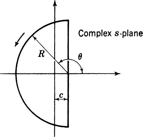
The line integral for F(t) is usually evaluated by transforming it into a closed contour and applying the calculus of residues discussed in Chap 1. The contour usually chosen is shown in Fig. 5.1.
Let us take as the closed contour Γ the straight line parallel to the axis of imaginaries and at a distance c to the right of it and the large semicircle s0 whose center is at (c, 0). We then have
where c is chosen great enough so that all the singularities of the integral lie to the left of the straight line along which the integral from c –j∞ to c +j∞ is taken.
The evaluation of the contour integral along the contour Γ is greatly facilitated by the use of Jordan’s lemma (Chap. 1, Sec. 15), which in this case may be stated in the following form:
Let ø(s) be an integrable function of the complex variable s such that
Then
It usually happens in practice that the function
Fig. 5.1
has such properties that Jordan’s lemma is applicable. In such a case the integral around the large semicircle in (5.2) vanishes as R→ ∞, and we have
Now, by Cauchy’s residue theorem (Chap. 1, Sec. 9), we have
Hence by (5.6) we have
if R is large enough to include all singularities.
If the function estg(s) is not single-valued within the contour Γ and possesses branch points within Γ, it may be made single-valued by introducing suitable cuts and then applying the residue theorem.
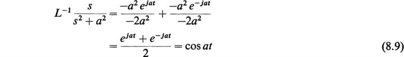
As an example of the computation of an inverse transform, let us consider the determination of the inverse transform of
This function clearly satisfies the condition imposed by Jordan’s lemma. Hence F(t) is given by (5.8) in the form
The poles of est/(s2 + a2) are at
Similarly we have
Hence
As another example, consider
This function also satisfies the condition of Jordan’s lemma. We must compute the sum of the residues of
The poles of this function are at
The sum of the residues at these poles is
To conclude this section let us state that once the function g(s) is known, its inverse may be readily evaluated, provided g(s) satisfies the conditions of Jordan’s lemma, by means of the residue theorem discussed in Sec. 12 of Chap. 1. Summarizing the results of the theory of residues as applied to (5.8) we may state that if g(s) has a simple pole at s = s0, then
or if g(s) has a pole of order n at s = s0, then
Thus these formulas may be used to evaluate the residues of g(s)est at all of its poles and through the application of (5.8) the inverse is found.
Let us consider the fundamental integral of the inverse transform
Now, if we perform a formal differentiation under the integral sign with respect to t, we have
and we see that differentiation introduces a factor of s before g(s). In many cases, however, the new integral does not converge uniformly.
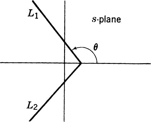
In such cases the process of differentiation cannot be performed in this manner, since for the operation to be valid the new integral must converge uniformly. It is possible, however, to modify the original integral in such a way that the procedure is correct. This may be done provided that g(s) satisfies certain conditions. The conditions, which are usually fulfilled in practice, are the following:
1. g(s) is analytic in the region to the right of the straight lines L1 and L2.
![]()
2. g(s) tends uniformly to zero as |s| → ∞ in this region (see Fig. 6.1).
It is possible, when these conditions hold, to complete the line integral by the way of a large semicircle convex to the left and with center at (c, 0) as before. Then, since no singularities are traversed, the path of integration may be changed into two straight lines L1 and L2, as shown in Fig. 6.1. This integral along L1 and L2 is called the modified integral.
The modified integral is easily proved uniformly convergent for all positive values of t. Also, integrals of the type
where Q(s) is a function that in the region under consideration increases at most as a power of s when s tends to infinity, may be proved uniformly convergent.
In Sec. 4 the relation
was derived.
We shall now remove the above restriction on m and obtain a general formula of the form
valid for all values of r.
Fig. 6.1
If we begin with the restricted result (6.4), we have
If m > – 1, the function
tends to zero uniformly as |s| → ∞. Hence we are permitted to differentiate (6.6) k times with respect to t under the integral sign.
We thus obtain
Hence we have
where
Now by the fundamental recursion formula of the gamma functions, we have
Therefore we may write (6.9) in the form
Now, if we let
we may write (6.12) in the form
for all values of r + 1 except negative integers. If r + 1 is a negative integer, let us place
We then have
This result follows from the fact that the integrand in (6.16) has no poles in the finite part of the s plane.
Although (6.16) holds for all values of r when t > 0, the inverse transforms of positive powers of s are not zero at t = 0 but are of the nature of impulsive functions.
The careful treatment of impulsive functions presents considerable difficulties and is beyond the scope of this discussion. However, many physical phenomena are of an impulsive nature. In electrical-circuit theory, for example, we frequently encounter electromotive forces that are impulsive in character, and we desire to study the behavior of the electric currents produced by the applications of electromotive forces of this type to linear circuits. In mechanics we frequently encounter problems in which a system is set in motion by the action of an impact or other impulsive force. Because of the practical importance of forces of this type, a simple treatment of them will be given.
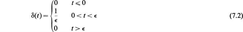
One of the most frequently encountered functions is the Dirac function δ(t). This function is defined to be zero if t ≠ 0 and to be infinite at t = 0 in such a way that
This is a concise manner of expressing a function that is very large in a very small region and zero outside this region and has a unit integral. Let us consider the function δ(t) that has the following values:
where ![]() may be made as small as we please. This function possesses the property (7.1).
may be made as small as we please. This function possesses the property (7.1).
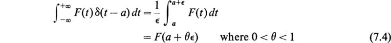
We now prove the following:
provided that F(t) is continuous. The proof of this follows from (7.2), so that we have
Now, since by hypothesis F(t) is continuous, we have
Hence the result (7.3) follows. As an application of (7.3), let us compute the Laplace transform of δ(t). We have
so that the Laplace transform of the Dirac function is 1.
As an example of the use of the δ(t) function, let us consider the effect produced when a particle of mass m situated at the origin is acted upon by an impulse F0 applied to the mass at t = 0. If the impulse acts in the x direction, the equation of motion is
Let
Now, if the mass is at x = 0 and t = 0 and has no initial velocity, we have
Hence Eq. (7.7) is transformed into
Therefore
and hence
As another example, consider a series circuit consisting of an inductance L0 in series with a capacitance C. Initially the circuit has zero current, and the capacitor is discharged. At t = 0 an electromotive force of very large voltage is applied for a very short time so that it may be expressed in the form E0 δ(t). It is required to determine the subsequent current in the system.
The differential equation governing the current in the circuit is
Now let
Therefore (7.13) transforms into
Hence
where
From the table of transforms we have
Hence
In Heaviside’s application of his operational method to the solution of physical problems, he made frequent and skillful use of certain procedures in order to interpret his “resistance operators.” These procedures were known as Heaviside’s rules in the early history of the subject. At that time there appears to have been much controversy over the justification of these rules. Viewed from the Laplacian-transform point of view, the proof of these powerful rules is seen to be most simple.
Heaviside’s first rule is commonly known as Heaviside’s expansion theorem, or the partial-fraction rule. In its usual form it may be stated as follows:
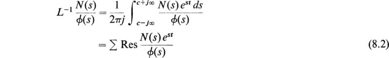
If g(s) has the form
where N(s) and ø(s) are polynomials in s and the degree of ø(s) is at least one higher than the degree of N(s) and, in addition, the polynomial ø(s) has n distinct zeros, s1 s2,. . . , sn, we then have
by the Cauchy residue theorem since in this case the integrand satisfies the conditions of Jordan’s lemma and the contribution over the large semicircle to the left of the path of integration vanishes as R → ∞.
We now compute the residues by the methods of Chap. 1, Sec. 12. Now if s1 s2, s3, . . . , sn are n distinct zeros of ø(s), then the points s = s1, s = s2, . . . , s = sn are simple poles of the function N(s)est/ø(s).
The residue at the simple pole s = sr is
where
It follows from (8.2) that
This result is called the Heaviside expansion theorem and is frequently used to obtain inverse transforms of the ratios of two polynomials. As a simple application of the expansion theorem, let it be required to determine the inverse transform of
In this case the zeros of ø(s) are
We also have
Hence, substituting in (8.5), we obtain
Heaviside’s expansion theorem as stated above is of use in evaluating the inverse transforms of ratios of polynomials in s. The expansion theorem is sometimes used to compute the inverse transforms of certain transcendental functions in s that have simple poles and that satisfy the conditions of Jordan’s lemma so that the path of integration may be closed to the left by a large semicircle. In this case the result
is applicable. If the poles of g(s) are simple poles at s = s1, s = s2, . . . , s = sn . . . , then Eq. (8.10) is very similar to the Heaviside expansion theorem (8.5).
As an example of this, consider the function
where T is real and positive. The poles of this function are at
or
The fact that these poles are simple poles follows from the fact that the derivative of scosh (Ts/2) with respect to s does not have zeros at these points. The function
satisfies the condition of Jordan’s lemma since
We thus have by (8.10)
since the residue at s = 0 is 0.
This expression reduces to
Substituting (8.13) into (8.17), we finally obtain
It is thus seen that the result (8.10) is more general than the Heaviside expansion theorem, but when applied to functions whose poles are simple, then (8.10) has a close resemblance to the Heaviside expansion theorem.
Heaviside made frequent use of the following result:
where the series ![]() is a convergent series of negative powers of s. This result is obtained by term-by-term substitution of
is a convergent series of negative powers of s. This result is obtained by term-by-term substitution of
since the series converges uniformly.
This concerns the transform of the series
By making use of the fact that
and the facts that
we have directly
By arranging the transform of a function in the form (8.21) Heaviside was able to obtain the asymptotic expansion of certain functions valid for large values of t.
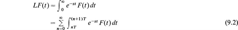
Let F(t) be a periodic function with fundamental period T, that is,
If F(t) is sectionally continuous over a period 0 < t < T, then its direct Laplace transform is given by
If we now let
and realize that, as a consequence of the periodicity of the function F(t), we have
in view of this we may write (9.2) in the form
We also have the well-known result
Hence we may write (9.5) in the form
Fig. 9.1
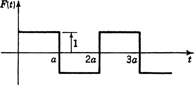
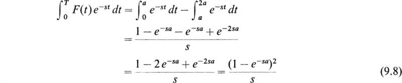
Let us apply this formula to obtain the transform of the “meander function” of Fig. 9.1. In this case we have
Hence, substituting this into (9.7), we have
Using the results of (8.18), we have
This is the Fourier-series expansion of the meander function.
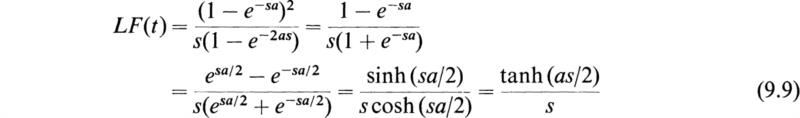
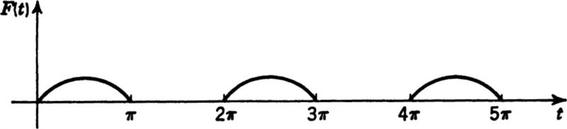
As another example, consider the function F(t) defined by
This function is given graphically by Fig. 9.2 and it is of importance in the theory of half-wave rectification. In this case the fundamental period is 2π. To obtain the transform of this function, we have
Hence, by Eq. (9.7), we obtain
Fig. 9.2
The method for solving differential equations mentioned in the heading of this section is essentially the same as that known under the name of Heaviside’s operational calculus. The modern approach to this method is based on the Laplace transformation. This method provides a most convenient means for solving the differential equations of electrical networks and mechanical oscillations.
The chief advantage of this method is that it is very direct and does away with tedious evaluations of arbitrary constants. The procedure in a sense reduces the solution of a differential equation to a matter of looking up a particular transformation in a table of transforms. In a way this procedure is much like consulting a table of integrals in the process of performing integrations.
Consider the functional relation between a function g(s) and another function h(t) expressed in the form
where s is a complex number whose real part is greater than zero and h(t) is a function such that the infinite integral of (10.1) converges and such that it satisfies the condition that
In most of the modern literature on operational, or Laplace-transform, methods the functional relation expressed between g(s) and h(t) is written in the following form:
The L denotes the “Laplace transform of” and greatly shortens the writing. The relation between h(t) and g(s) is also written in the form
In this case we speak of h(t) as being the inverse Laplace transform of g(s).
Let us suppose that we have the functional relation
or, symbolically,
Let us now determine L(dx/dt) in terms of y(s). To do this, we have
By integrating by parts we obtain
Now, if we assume that
and that
![]()
exists when s is greater than some fixed positive number, then (10.8) becomes
where
Equation (10.10) gives the value of the Laplace transform of dx/dt in terms of the transform of x and the value of x at t = 0.
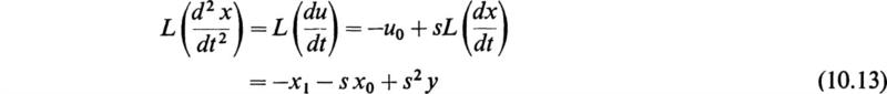
In order to compute the Laplace transform of d2x/dt2, let
Then in view of (10.10) we have
where x1 is the value of dx/dt at t = 0.
Repeating the process, we obtain
and
where
The above formulas for the transforms of derivatives are of great importance in the solution of linear differential equations with constant coefficients.
To illustrate the general theory, let it be required to solve the simple differential equation
subject to the initial condition that
To solve this by the Laplace-transform method, we let
and use (10.10); then, in terms of y, the equation becomes
or
The solution of one equation could be written symbolically in the form
Consulting the table of transforms in Appendix A, we find that transform 1.1 gives
Accordingly we have
as the solution of the differential equation (10.19) subject to the given initial conditions.
As another example, let us solve the equation
subject to the initial conditions that
As before, we let y = Lx and replace every member of (10.20) by its transform. Consulting the table of transforms, we find from No. 2.5 that
Using (10.13), Eq. (10.20) is transformed to
or
Consulting the table of transforms in Appendix A, we find that Nos. 2.4, 2.5, and 4.10 give the required information, and we have
as the required solution.
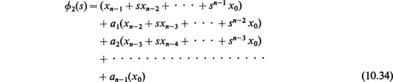
To solve the general equation with constant coefficients
we introduce y = Lx and φ1(s) = LF(t) and replace the various derivatives of x by their transforms given by (10.16). We then obtain
If we write
Eq. (10.33) may be written concisely in the form
To obtain the solution of the differential equation (10.32), we must obtain in some manner the inverse transform of y(s), and we would then have
If F(t) is a constant, eat, cosωt, sinωt, tn where n is a positive integer, eat sinωt, eat cosωt, tneat, tncosωt, or tnsinωt, then ø1(s) is a polynomial in s. The procedure in such a case is to decompose the expressions ø1(s)/Ln(s) and ø2(s)/Ln(s) into partial fractions, examine the table of transforms, and obtain the appropriate inverse transforms.
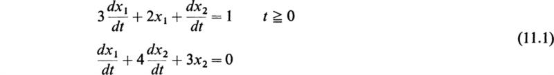
In the study of dynamical systems, whether electrical or mechanical, the analysis usually leads to the solution of a system of linear differential equations with constant coefficients. The Laplace-transform method is well adapted for solving systems of equations of this type. The method will be made clear by an example. Consider the system of linear differential equations with constant coefficients given by
Let us solve these equations subject to the initial conditions
To solve these equations by the Laplace-transform method, let
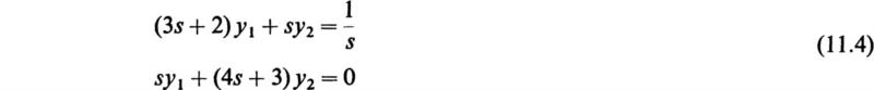
Then, in view of (10.10) and the fact that the Laplace transform of unity is 1, the equations transform to
Solving these two simultaneous equations for y1, we obtain
Using the transform pair No. 3.5 of the table (Appendix A), we obtain
Solving for y2, we have
By the use of the transform pair No. 2.2, we obtain
This example illustrates the general procedure. In Chaps. 5 and 6 the systems of differential equations arising in the study of electrical networks and mechanical oscillations are considered in detail.
Further examples To further illustrate the use of the table of Laplace transforms in the solution of differential equations, the following examples are appended.
1 Suppose it is required to solve the equation
![]()
subject to the initial conditions

To solve the equation, we let
![]()
By the basic theorem (III) we have
![]()
and by No. 1.1 (Appendix A)
![]()
The equation to be solved is thus transformed to
![]()
Therefore
![]()
Using Nos. 3.16 and 2.4, we have the inverse transform of Y(s):
![]()
This is the required solution.
2. A constant electromotive force E is applied at t = 0 to an electrical circuit consisting of an inductance L, resistance R, and capacitance C in series. The initial values of the current i and the charge on the capacitor q are zero. It is required to find the current.
The current is given by the equation
![]()
where ![]()
NOTE : The script ![]() is used to denote the Laplace transform in order not to confuse it with the inductance parameter L.
is used to denote the Laplace transform in order not to confuse it with the inductance parameter L.
By (III) the equations are transformed to

There we have
![]()
Therefore
![]()
where
![]()
By No.2.12 we have
![]()
or by no.18

3. Resonance of a pendulum A simple pendulum, originally hanging in equilibrium, is disturbed by a force varying harmonically. It is required to determine the motion. The differential equation is
![]()
Let the pendulum start from rest at its equilibrium position. In such a case we have the initial conditions
![]()
Let Lx = y; then by (III) L![]() = s2y. Using No. 2.4, the differential equation of motion is transformed to
= s2y. Using No. 2.4, the differential equation of motion is transformed to
![]()
or
![]()
By No.2.4 we obtain
![]()
and by No. 4.9
![]()
4. Differential equation with variable coefficients As the final example let us consider the differential equation
![]()
which is a standard form of Bessel’s equation (cf. Appendix B). If we let
![]()
then
![]()
and
![]()
and hence
![]()
Taking the Laplace transform of the original differential equation yields
![]()
Integrating this equation once with respect to s and setting the constant of integration to zero† gives
![]()
This equation is separable, and performing this operation gives
![]()
Integrating this equation yields
![]()
or
![]()
Using the table of transforms in Appendix A, we may find the inverse of the above expression from entry R-B.l which gives
![]()
which is a Bessel function of the first kind of order zero.
The reader may also recall that the inverse of the above result for Y(s) was computed by means of evaluating the inversion integral via integration in the complex plane as the second example in Chap. 1, Sec. 18.
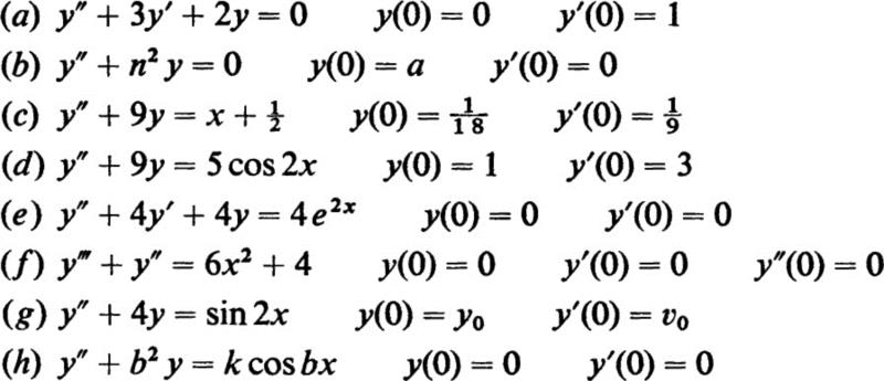
Solve the following equations:

5. Find the solution of the following equations which satisfy the given initial conditions:
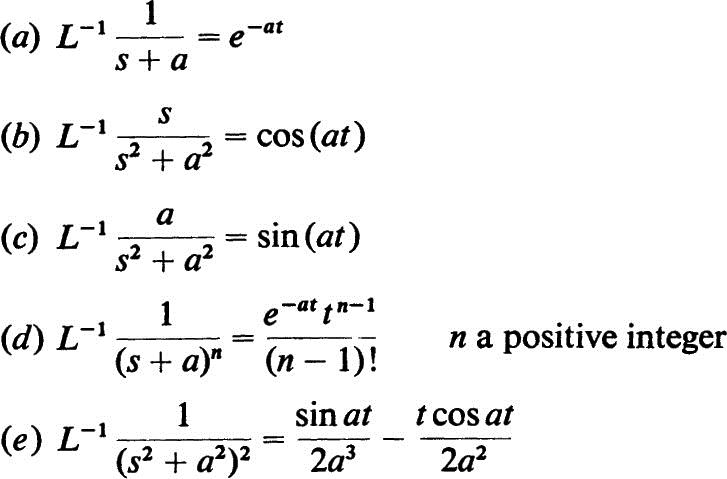
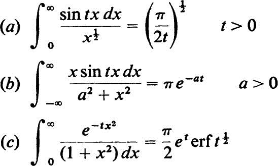
6. Using the complex line integral of the Fourier-Mellin transformation, show that the following inverse transforms have the indicated values:
7. Solve the transforms in Prob. 6 by use of the residue theorem.
![]()
by expanding the left side into a series of inverse powers of s and inverting term by term to obtain the series expansion for J0(at).
![]()
is the meander function given in Fig. 9.1.
10. Evaluate the following integrals operationally:
11. Evaluate the Laplace transforms of the following functions by direct integration of the transform integral:
![]()
12. Solve the following homogeneous equations:
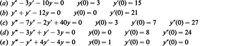
(Hochstadt, 1964, see reference in Chap. 2)
13. Solve the following differential equations:
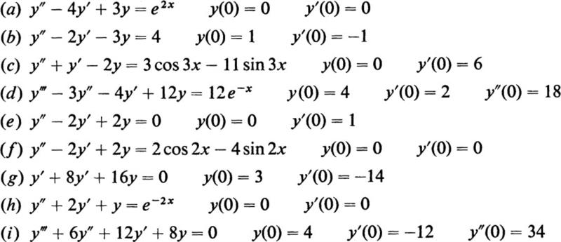
(Kreyszig, 1962, see reference in Chap. 2)
14. Following Theorem XIII, derive a relation for Ltÿ(t) when y(0) and ![]() are not zero.
are not zero.
1. Davis, H. T.: “The Theory of Linear Operators,” The Principia Press, Bloomington, Ind., 1936.
2. Whittaker, E. T.: Oliver Heaviside, Bulletin of the Calcutta Mathematical Society,vol. 20, p. 199, 1928–1929.
3. Laplace, P. S.: Sur les suites, oeuvres complètes, Mémoires de l’academie des sci., vol. 10, pp. 1–89, 1779.
4. Carson, J. R.: “Electric Circuit Theory and the Operational Calculus,” McGraw-Hill Book Company, New York, 1926.
5. Jeffreys, H.: “Operational Methods in Mathematical Physics,” Cambridge University Press, New York, 1931.
6. Carslaw, H. S., and J. C. Jaeger: “Operational Methods in Applied Mathematics,” Oxford University Press, New York, 1941.
7. McLachlan, N. W.: “Modern Operational Calculus,” The Macmillan Company, New York, 1948.
8. McLachlan, N. W.: “Complex Variable Theory and Transform Calculus,” Cambridge University Press, New York, 1953.
9. Gardner, M. S., and J. L. Barnes: “Transients in Linear Systems,” John Wiley & Sons, Inc., New York, 1942.
10. Thomson, W. T.: “Laplace Transformation Theory and Engineering Applications,” Prentice-Hall, Inc., New York, 1950.
11. van der Pol, B., and H. Bremmer: “Operational Calculus,” Cambridge University Press, New York, 1950.
12. Pipes, L. A.: The Operational Calculus, Journal of Applied Physics, vol. 10, nos. 3–5, 1939.
13. Denis-Papin, M., and A. Kaufmann: “Cours de calcul opérationnel,” Editions Albin Michel, Paris, 1950.
14. Doetsch, G.: “Theorie und Anwendung der Laplace-Transformation,” Springer- Verlag OHG, Berlin, 1947.
15. Wagner, K. W.: “Operatorenrechnung,” J. W. Edwards, Publisher, Inc., Ann Arbor, Mich., 1944.
16. Jaeger, J. C: “An Introduction to the Laplace Transformation,” John Wiley & Sons, Inc., New York, 1949.
17. Churchill, R. V.: “Modern Operational Mathematics in Engineering,” McGraw-Hill Book Company, Inc., New York, 1944.
18. van der Pol, B., and K. F. Niessen: Symbolic Calculus, Philosophical Magazine, vol. 13, pp. 537–577, March, 1932.
19. Sears, W. R.: Operational Methods in the Theory of Airfoils in Non-uniform Motion, Journal of the Franklin Institute, vol. 230, pp. 95–111, 1940.
20. Pipes, L. A.: The Analysis of Retarded Control Systems, Journal of Applied Physics, vol. 19, no. 7, pp. 617–623, 1948.
21. Gross, B.: On Creep and Relaxation, Journal of Applied Physics, vol. 18, no. 2, pp. 212–221, 257–264, 1947.
22. van der Pol, B.: Application of the Operational or Symbolic Calculus to the Theory of Prime Numbers, Philosophical Magazine, ser. 7, vol. 26, pp. 912–940, 1938.
23. Heaviside, Oliver: “Electromagnetic Theory,” Dover Publications, Inc., New York, 1950.
24. Pipes, L. A.: The Summation of Fourier Series by Operational Methods, Journal of Applied Physics, vol. 21, no. 4, pp. 298–301, 1950.
25. Jaeger, J. C: The Solution of Boundary Value Problems by a Double Laplace Transformation, Bulletin of the American Mathematical Society, vol. 46, p. 687, 1940.
26. Voelker D., and G. Doetsch: Die zweidimensionale Laplace-Transformation,” Verlag Virkhauser, Basel, 1950. [Contains an extensive table of two-dimensional Laplace transforms.]
27. Estrin, T. A., and T. J. Higgins: The Solution of Boundary Value Problems by Multiple a place Transformations, Journal of the Franklin Institute, vol. 252, no. 2, pp. 153–167, 1951.
28. Pipes, L. A.: An Operational Treatment of Nonlinear Dynamical Systems, Journal of he Acoustical Society of America, vol. 10, pp. 29–1, 1938.
29. Pipes, L. A.: Operational Analysis of Nonlinear Dynamical Systems, Journal of Applied Physics, vol. 13, no. 2, February, 1942.
30. Pipes, L. A.: The Reversion Method for Solving Nonlinear Differential Equations, Journal of Applied Physics, vol. 23, no. 2, pp. 202–207, 1952.
31. Pipes, L. A.: Operational Methods in Nonlinear Mechanics, Report 51–10, University of California, Los Angeles, 1951.
32. Pipes, L. A.: Applications of Integral Equations to the Solution of Nonlinear Electric Circuit Problems, Communication and Electronics, no. 8, pp. 445–450, September, 1953.
33. McLachlan, N. W., and P. Humbert: Formulaire pour le calcul symbolique, Memorial des sciences mathématiques, fasc. 100, 1941.
34. Erdelyi, A. (ed.): “Tables of Integral Transforms,” vol. I, McGraw-Hill Book Company, New York, 1954.
35. Fodor, G.: “Laplace Transforms in Engineering,” Akademiai Kiado, publishing house of the Hungarian Academy of Sciences, Budapest, 1965.
36. Roberts, G. E., and H. Kaufman: “Table of Laplace Transforms,” W. B. Saunders Company, Philadelphia, 1966.
37. Ryshik, I. M., and I. S. Gradstein: “Tables of Series, Products, and Integrals,” 2d ed., VEB Deutscher verlag der Wissenschaften, Berlin, 1963.
38. McCollum, P. A., and B. F. Brown: “Laplace Transform Tables and Theorems,” Holt, Rinehart and Winston, Inc., New York, 1965.
† In this chapter we shall deviate from our usual method of indicating references and denote them by bracketed numbers which are keyed to the references at the end of this chapter.
† A rigorous discussion and derivation of this theorem will be found in E. C. Titchmarsh “Introduction to the Theory of Fourier Integrals,” Oxford University Press, New York, 1937.
† The setting of this arbitrary constant to zero simply eliminates the second solution to the original equation.