It is fairly safe to state that the subject of complex variables is fundamental to the subject of applied mathematics. A solid background in this area is essential for the application of many useful methods of analysis to obtain solutions to a wide range of practical problems.
This chapter is intended as a review and brief summary of many of the useful results of complex function theory. It has been assumed by the authors that the reader has some familiarity with complex numbers.† A more thorough coverage of this topic can be found in any of the references at the end of this chapter.
From the basic theory of complex numbers it may be shown how the elementary transcendental functions, for example, sin x, cos x, ex, and so on, are defined for complex values of their arguments simply by allowing the variable in the power series expansions of these functions to take on complex values, for example, sin z, cos z, ez, and so on. Any function of the complex variable
is termed a complex function and is frequently expressed in the following form:
In this expression the functions u and υ are real functions of the real variables x and y. Just as x and y are the real and imaginary parts of z, u(x, y) and υ (x, y) are the real and imaginary parts of the complex function w(z) :
As specific examples consider the complex functions sin z and ez. The real and imaginary parts may be found as follows:
where use has been made of the well-known formulas
From (2.4) we find that
For ez we have
from which we find that
In deriving (2.7) we have made use of the first of the following three Euler formulas:
Let us now consider the expression
and determine what conditions it must satisfy in order that it may be a function of z. If we speak in the broadest sense of the word function, then w is always a function of z since if z is given then x and y are determined and it follows that u and υ are determined in terms of x and y.
This definition is too broad, and in the theory of functions of a complex variable it is restricted by demanding that the function w shall have a definite derivative for a given value of z.
It must be realized that if w(z) is one of the analytic elementary transcendental functions, such as zn, sin z, cosh z, ln z, etc., this condition is usually met since many of the operations used in the calculus of real variables to obtain the derivatives are still valid for the complex variable and hence the derivative is uniquely determined. We thus have
However, it will now be shown that the uniqueness of the derivative requires the functions u and υ to satisfy certain conditions.
In the theory of functions of a real variable, if the difference quotient
where F(x) is a real function of the real variable x, can be resolved into two terms in such a way that the first is independent of h and the second one is such that
then by definition it is possible to differentiate F(x), and F′(x) is called the derivative of F(x). Hence
This definition is transferred to complex functions as follows:
Fig. 3.1
where
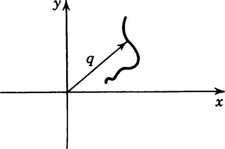
In this case, however, q represents a vector in the xy plane of Fig. 3.1. The end point of the vector representing the complex number q can converge toward the origin as q → 0 along any arbitrary curve. The derivative w′(z) is defined by
and must be independent of the manner in which q approaches zero in order to be unique.
In order to carry out the limiting process (3.6), let
and
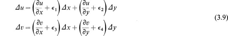
Now, since u and υ are functions of x and y, then, if u and υ have continuous partial derivatives of the first order, we have
where
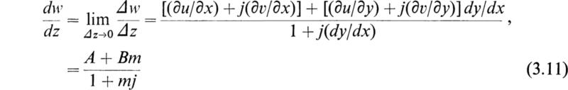
Substituting (3.7), (3.8), and (3.9) in (3.6), we have
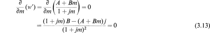
Now, if dw/dz is to be unique, it must be independent of the manner in which ∆z approaches zero and hence must be independent of m = dy/dx. If dw/dz = w′ is independent of m, we must have
Hence
or
Equating the coefficients of the real and imaginary terms of (3.15), we obtain (3.16)
and
Equations (3.16) and (3.17) are the conditions that the real and imaginary parts of w(z) must satisfy in order that w(z) may have a unique derivative w′(z). Such a function is said to be analytic at the point z. These equations are called the Cauchy-Riemann differential equations. We thus see that the real and imaginary parts of an analytic function satisfy Cauchy-Riemann differential equations. Conversely, it is easily verified that, if the real and imaginary parts have continuous first partial derivatives satisfying Cauchy-Riemann differential equations, then the function is analytic.
If we differentiate Eq. (3.16) with respect to y and Eq. (3.17) with respect to x and add the results, we obtain
Differentiating (3.17) with respect to y and (3.16) with respect to x and subtracting the results, we obtain
Thus we see that the real and imaginary parts of an analytic function w(z) of a complex variable are solutions of the two-dimensional Laplace equation. It is therefore true that w(z) is itself a solution to Laplace’s equation.
The functions u and υ that satisfy the Cauchy-Riemann equations (3.16) and (3.17) are called conjugate functions. It is also true that if one of these functions is known, the other may be found to within an arbitrary constant by integrating the Cauchy-Riemann equations. This implies that w(z) may be determined to within an arbitrary complex constant. As an example let us consider that u is given and it is desired to find the conjugate function υ. Assuming that
and integrating (3.17) yields
Now, if we integrate (3.16) we find
Comparing (3.21) and (3.22), it may be deduced that
where c" = a constant.
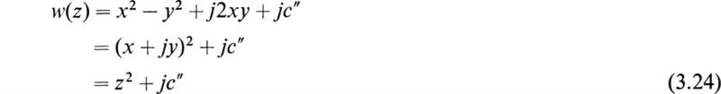
If Eqs. (3.20) and (3.23) are substituted into (2.2) there results
It should be mentioned at this point that once Eq. (3.21) has been obtained the result could have been substituted into Eq. (3.16) to yield a first-order differential equation for the undetermined function c(x). This method is more direct but requires the solution of a first-order differential equation.
In a large number of applications only the derivatives of w(z) are required and therefore the arbitrary constant may be dropped.
Substituting Eqs. (3.16) and (3.17) into (3.11) yields
The use of these functions in the solution of two-dimensional potential problems will be discussed in Chap. 9.
The concept of the line integral of a vector field is familiar to those who have had a brief introduction to vector algebra. In this chapter the concept of a line integral of a complex function will be developed.
Let w(z) be a complex function of the complex variable z defined in the region B (Fig. 4.1), and let C be a smooth curve in the region B having end point z0 and z. Let z1, z2, z3, . . , zn–1 be an arbitrary number of intermediate points on C and zn chosen to be the point z.
Let
represent chord vectors of the curve C. Let mr be a point on the curve C located between zr–1 and zr (this point may also coincide with zr–1 or with zr). Let the following summation be performed:
If the curve C is divided into smaller and smaller parts so that n→ ∞, |∆zr|0, and if the summation tends to a limit that is independent of the choice of the intermediate points and of the manner in which the division is performed, then the above limit Ln is called the definite integral of the complex
Fig. 4.1
function w(z) taken along the path C and between the limits z = z0 and z = z and is denoted by
As in the case of real quantities, it may be shown that the limit Ln exists if w(z) is continuous along the path of integration.
The value of this integral in general depends on w(z) and on the limits of the integral as well as on the form of the path C.
Let the curve C be a curve of finite length (rectifiable curve); then, if
where M represents a fixed real quantity throughout the curve C, the following estimation of the integral along the curve C exists,
where s is the length of the curve C from z0 to z.
To prove (4.5), we substitute (4.4) in Eq. (4.2) and obtain
However,
This proves Eq. (4.5).
If we decompose w(z) into its real and imaginary parts
and write
we have
where we now have two real line integrals.
Let the function w(z) be single-valued and continuous and possess a definite derivative throughout a region R; that is, let w(z) be analytic in R.
Cauchy’s integral theorem states that
where the above notation signifies that the line integral is taken along an arbitrary closed path lying inside the region R.
The proof of this theorem can be made to depend on Stokes’s theorem of Appendix E, Sec. 10. Stokes’s theorem states that, if we have a vector field A whose components possess the continuous partial derivatives involved in the calculation of ∇ × A, then
where the line integral is taken along the curves bounding the open surface s. If A is a two-dimensional vector field having the components Ax and Ay above, then (5.2) reduces to
where c is a closed curve lying in the xy plane and s is the surface bounded by this curve. As a consequence of (4.10) we may write
By means of (5.3) we may transform both the integrals of the right-hand member of (5.4) into surface integrals. To transform the first one, let
We thus obtain
However, as a consequence of the first Cauchy-Riemann equation (3.16), we have
Hence the first integral of the right-hand member of (5.4) vanishes. Using Eq. (5.3) to transform the second integral of the right-hand member of (5.4) and the second Cauchy-Riemann equation (3.16), this integral may be shown to vanish also. Hence Cauchy’s integral theorem (5.1) is proved.
Fig. 5.1
As a consequence of this theorem it follows that the path of the line integral, whether closed or between fixed limits, may be deformed without changing the value of the integral, provided that in the deformation no point is encountered at which w(z) ceases to be analytic.
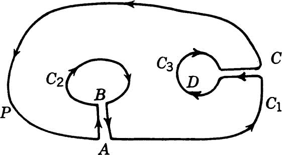
Cauchy’s integral theorem has been deduced under the assumption that the closed curve is the boundary of a simply connected region. However, as we shall see, the theorem still holds if the enclosed region is multiply connected. Consider the region of Fig. 5.1.
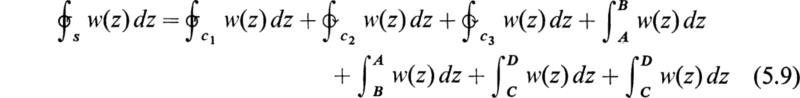
This region requires three curves c1, c2, and c3 to divide it into two separate parts and is therefore a triply connected region. By introducing the crosscuts AB and CD the region may be transformed into a simply connected region. We thus have
where the curve s includes the outer curve c1 traversed in the mathematically positive direction, the curves c2 and c3 traversed in the negative direction, and the crosscuts AB and CD. We thus have
Since the function is analytic along the crosscuts and the integral from A to B is traversed in the opposite direction from the integral B to A, etc., the integrals along the crosscuts cancel out in pairs. Using this fact and transposing, we obtain
where we have reversed the direction of integration along curves c2 and c3.
Fig. 5.2
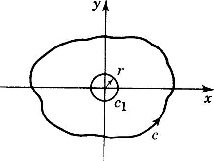
As an example of the use of Cauchy’s integral theorem, let it be required to compute the integral
where c is a simple closed curve.
The function w(z) = 1/z is analytic for any value of z except for z = 0. If, therefore, the simple closed curve c encloses the origin, let us draw an arc c1 of small radius r with center at the origin as shown in Fig. 5.2.
Since the function 1/z is analytic in the region between c1 and c, we have by Eq. (5.10)
Now on the circle c1 we have
Hence
We thus have the result
The implication of Cauchy’s integral theorem is that, provided no singularities are crossed, any contour integral may be deformed into any other. As seen in the example above, the contour c was deformed into the contour c1.
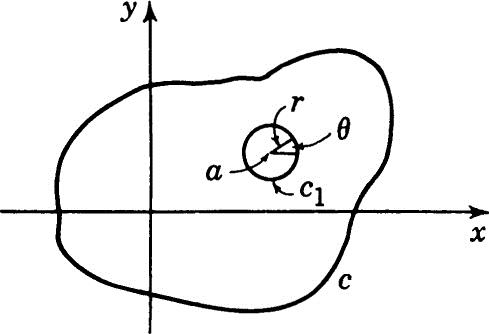
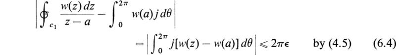
Let w(z) be analytic in a region including a point z = a and bounded by a curve c. Let us draw a small circle c1 of radius r and center at a, as shown in Fig. 6.1.
Fig. 6.1
Then, in the area bounded by the circle c1 and the curve c, the function
is analytic. Hence, by Cauchy’s theorem, we have
Now on the circle c1 we have
By continuity of w(z) we may make |w(z) — w(a)| < ![]() , for any given
, for any given ![]() > 0 making r sufficiently small. Hence
> 0 making r sufficiently small. Hence
Since by (5.10) the integral on the right may be evaluated on any circle enclosing a and since w(z) is continuous at a, it can be made arbitrarily small in magnitude. In other words,
Hence, from (6.4) and (6.2), we obtain
or
This is Cauchy’s integral formula; it is remarkable in that it enables one to compute the value of a function w(z) inside a region in which it is analytic from the values of the function on the boundary.
If we apply the formula to a circle with center at a of radius R, we have
and we obtain
This shows that the value of the function w(z) at the center of a circle is equal to the average value of its boundary values. If M denotes the maximum of the absolute value of w(z) on the boundary of the circle, then
Hence
Therefore the maximum of the absolute value of an analytic function cannot be situated inside a circular region.
It is of interest to note that since w(z) = u +jυ, the above relations derived for w(z), that is, Eqs. (6.9) and (6.10), also hold for u and v separately. Thus we may infer that solutions of Laplace’s equation must satisfy the stated relations. This means that the values of the solutions to Laplace’s equation may be computed by an integration over the boundary conditions via Eq. (6.7).
The feature that the value of a solution at the center of a circular region is the average of the boundary conditions has great significance for obtaining numerical solutions to Laplace’s equation which should be familiar to those with some background in numerical analysis.
Another form of Cauchy’s integral formula is obtained by replacing a by z and letting z = t in (6.7). We then have
where now z is held fixed in the integration and t traverses the curve c.
It may be shown that the integral (6.12) may be differentiated under the integral sign and that the result thus obtained may be differentiated in the same way. This will be assumed. Then we have
From this it follows that if a function is analytic all its derivatives exist. This is not necessarily true of a function of a real variable.
The Taylor’s series expansion of a function of a real variable should be quite familiar to those who have had only a slight background in differential calculus. By means of Cauchy’s integral formula we may develop the Taylor’s series expansion of a function of a complex variable. Let us consider the function w(z) and let z be replaced by z + h in Eq. (6.12), which yields
where we assume that w(z) is analytic in a circle R with the boundary c and that the points z and z + h are inside of this circle. Let us now expand 1/[t – (z + h)] into a power series in h in the form
Hence
Using (6.15) and (6.1), we have
where Rn+1 is the remainder after n + 1 terms and is given by
Now, by the estimation formula (4.5), it may be shown that
The series (7.4) converges inside of a circle with z as its center, the radius of the circle being equal to the distance from z to the nearest point z + h at which w(z + h) is no longer analytic. Series (7.4) may also be represented as follows:
where
Thus the coefficients may be obtained by means of integration.
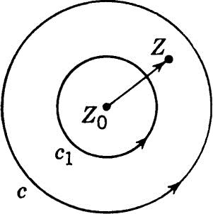
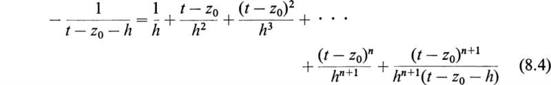
Let w(z) be an analytic function in the annular region of Fig. 8.1 including the boundary of the region. The annular region is formed by two concentric circles c and c1 whose center is z0. Let z0 + h = z be located inside the annular region. If we apply Cauchy’s integral theorem to this annular region, we have
The integration is carried out over the entire boundary of the annular region composed of the circles c and c 1 We thus have symbolically
where the integration over both circles must be taken in the positive direction. Each integral is calculated individually. Now, as in Eq. (7.2), we have
Fig. 8.1
If we interchange t – z0 and h, we have
If we now substitute these expansions in Eq. (8.2), we have
where
By Cauchy’s estimation formula (4.5) it is easy to show that
Hence we obtain the Laurent’s series
where the coefficients as are given by (8.6) and (8.7). It may be noted that if all the coefficients of negative index have the value zero, then (8.10) reduces to Taylor’s series.
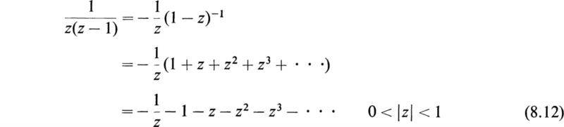
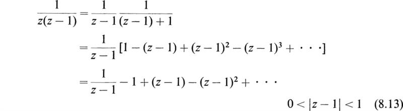
Consider the function
This function is analytic at all points of the z plane except at the points z = 0 and z = 1. Therefore it is possible to expand this function in a Laurent’s series in an annular region about z = 0 or z = 1.
To expand about z = 0, we have
To expand about z = 1, write
As another example, consider the function
This function may be expanded in any annular region enclosing the origin in the form
In this case all the terms of the Laurent’s series have a negative index.
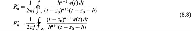
In the Laurent’s series (8.10) let
We then obtain
The coefficient a–1 is given by Eq. (8.7), and it is
where c1 is a curve surrounding the point z0. a–1 is in general a complex number and is called the residue of w(z) at the point z = z0. It is usually denoted by
It sometimes happens that the Laurent’s series for w(z) is known in the neighborhood of z = z0, or the series is easier to compute than the integral. In this case from a knowledge of a–1 we may compute the integral (9.3).
As a very simple example, consider the function w(z) = 1/z. In this case the Laurent’s series about the origin consists of only one term, and we have
Hence
where the integral is taken about a curve surrounding the origin. In the same manner we have
where the path of integration encloses the origin. This follows from the expansion of the function e1/z in the series (8.15): Hence we see that
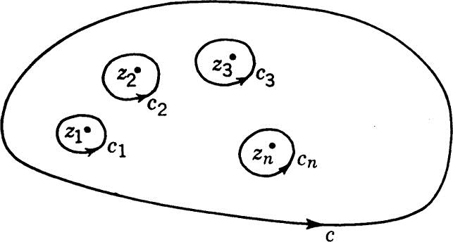
Let w(z) be an analytic function inside a region R at all points except at the points z1, z2, . . . , zn. Let w(z) be analytic at all points on the boundary c of the region R. Let us surround the points z1, z2, . . . , zn by the closed curves c1, c2, . . , cn. Then by Cauchy’s integral theorem of Sec. 5, we have (see Fig. 9.1)
Fig. 9.1
However, by (9.3), we have
Hence, substituting this in (9.9), we obtain
This is Cauchy’s residue theorem. It is of extreme importance in evaluating definite integrals and in the theory of functions in general. Applications of this theorem to the evaluation of definite integrals will be considered in a later section.
All the points of the z plane at which an analytic function does not have a unique derivative are said to be singular points. They are the points at which the function ceases to be analytic. If we concern ourselves only with single-valued functions of the complex variable w(z), then w(z) may have two types of singularities:
1. Poles, or nonessential singular points
2. Essential singular points
The distinction between these two types of singularities will now be explained.
Let z0 be a singular point of w(z). Let us expand w(z) in a Laurent’s series in powers of z – z0. This expansion will contain powers of z – z0 with negative exponents, for otherwise z = z0 would not be a singular point. Hence we have
There are two possibilities:
a. The expansion (10.1) has only a finite number of powers of z – z0 with negative exponents.
In this case w(z) is said to have a pole at z = z0. If m is the largest of the negative exponents and if the function
behaves regularly (is analytic) and is not zero at the point z0, m is called the order of the pole z0 and w(z) is said to have a pole of the mth order at the point z0.
The sum of the terms with negative exponents
is called the principal part of the function w(z) at z0.
b. The other possibility is that the Laurent’s expansion of the function w(z) about the point z0 will have an infinite number of negative powers of z – z0 and is of the form
In this case the point z = z0 is said to be an essential singular point, and w(z) is said to have an essential singularity at z = z0.
As examples of these possibilities, consider the function
This function has a pole of the second order at z = 2, a pole of the third order at z = 5, and a pole of the first order at z = 1.
has the Laurent’s series (8.15) in the neighborhood of the origin. Its Laurent’s-series expansion contains an infinite number of negative powers of z and has, therefore, an essential singularity at z = 0.
If a function w(z) has poles only in the finite part of the z plane, it is said to be a meromorphic function.
In the theory of the complex variable it is convenient to regard infinity as a single point. The behavior of w(z) “at infinity” is considered by making the substitution
and examining w(1/t) at t = 0. We then say that w(z) is analytic or has a pole or an essential singularity at infinity according as w(1/t) has the corresponding property at t = 0.
It may thus be shown that 1/z2 is analytic at infinity, z3 has a pole of the third order at infinity, and the function
has an essential singularity at infinity.
The residue of w(z) at infinity is defined as
where c is a large circle that encloses all the singularities of w(z) except at z =∞. The integration is taken around c in the negative sense, that is, negative with respect to the origin, provided that this integral has a definite value.
If we apply the transformation
to the integral (11.3), it becomes
where the integration is performed in a positive sense about a small circle whose center is at the origin. It follows that, if
has a definite value, then that value is the residue of w(z) at infinity.
For example, the function
behaves like 1/z for large values of z and is therefore analytic at z= ∞. However,
Hence the residue of w(z) at infinity is –1. We thus see that a function may be analytic at infinity and still have a residue there.
The calculation of the residues of a function w(z) at its poles may be performed in several ways. By the definition of the residue of the function w(z) at a simple pole z = z0 is meant the coefficient a–1 in the Laurent’s expansion of w(z) in the form
where z0 is a simple pole. If we now multiply Eq. (12.1) by z – z0 and take the limit z → z0, we have
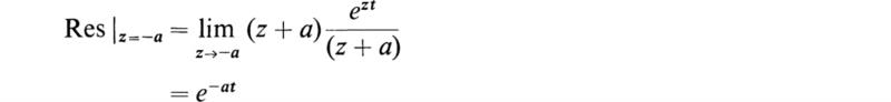
For example, the function
has two simple poles, one at z = ja and another at z = –ja. To evaluate the residue at z = ja, we form the limit
Similarly, the limit at z = –ja is —e–ja/2ja.
RESIDUES AT SIMPLE POLES OF w(z) = F(z)/G(z)
Frequently it is required to evaluate residues of a function w(z) that has the form
where G(z) has simple zeros and hence w(z) has simple poles. If z = z0 is a simple pole of w(z), then by (12.2) we have
Since z = z0 is a simple pole of w(z), we must have
so that expression (12.6) becomes 0/0. To evaluate it, we use L’Hospital’s rule and obtain
As an example of the use of this formula, let it be required to compute the residue of w(z) = ejz/(z2 + a2) at the simple pole z =ja. Using (12.8), we have
If the function w(z) has a multiple pole at z = z0 of order m, then the Laurent’s expansion of w(z) is
The residue at z = z0 is a–1, and to obtain it we multiply (12.10) by (z – z0)m and obtain
If we differentiate both sides of (l2.11), with respect to z, m – 1 times and place z = z0, we obtain
Hence the residue a–1 at the multiple pole is
For example, let it be required to find the residue of
at the third-order pole z = a. Applying (12.13), we have
A very interesting and useful theorem may be established by the aid of the notion of residues. Let w(z) be a function that is analytic at all points of the complex z plane and finite at infinity. Then, if a and b are any two distinct points, the only singularities of the function
are a and b and possibly infinity. However, since w(z) is by hypothesis finite at infinity, we have
Hence the residue of ø(z) is zero at infinity. However, in Sec. 11 we saw that the residue ø(z) at infinity is defined by
where c is a large circle that encloses all the singularities of ø(z) except the one at z = ∞ and the integration is performed in the negative sense. However, by Cauchy’s residue theorem, we have
Hence the sum of the residues of ø(z), including that at infinity, is zero. Now the residue of ø(z) at z = a is
and, similarly, the residue at z = b is w(b)/(b – a). Since the sum of the residues vanishes, we have
Hence
and since a and b are arbitrary points, w(z) is a constant. We have thus proved Liouville’s theorem, which states:
A function that is analytic at all points of the z plane and finite at infinity must be a constant.
As a corollary of this theorem, it follows that every function that is not a constant must have at least one singularity.
It also follows that if w(z) is a polynomial in z, the equation
has a root, because if it had not, the function l/w(z) would be finite and analytic for all values of z and would therefore be a constant; then w(z) would be a constant. This contradicts the original hypothesis. This is the fundamental theorem of algebra.
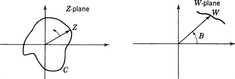
A theorem due to Cauchy will now be discussed. This theorem is very useful in determining the number of zeros and poles of a function W(z) within a closed contour by an inspection of the behavior of the function W(z) itself as the point z traverses the given contour. The results of the theorem can be applied to the problem of determining the approximate location of the roots of algebraic equations.
Consider the function W(z) that has both zeros and poles within some prescribed contour C of the z plane and no other singularities. Let
If we differentiate (13.9) with respect to z, we have
Now let z0 be either a zero of the nth order of W(z) or a pole of the nth order of 1/W. In such a case we can write
where the function g(z) is analytic and nonzero at z = z0 and n is a positive integer if z0 is a zero of W(z) or n is a negative integer if z0 is a pole of W(z).
Let (13.11) be differentiated with respect to z. We then have
Hence
Equation (13.13) shows that the function (1/W)(dW/dz) has a simple pole at z0 and the residue at this pole is n. Now consider the closed contour C and the integral (13.13):
Fig. 13.1
It is apparent from (13.12) and (13.13) that
where N is the total number of zeros and P the total number of poles of W(z) within the closed contour C, provided multiple zeros and poles are weighted according to their multiplicity. Now
Where ∆c ln W(z) is the change in ln W(z) as the closed contour C is traversed. But
by (13.9), where arg W(z) is the argument of W(z). But ln |W(z)| is a single-valued function. Hence
Combining the results of (13.15), (13.16), and (13.18), we get
or
where ∆cB indicates the change in B as the closed contour C is traversed. As the point z moves in the z plane and traces the contour C, the point W moves in the W plane, tracing another contour. B is the angle that the representative vector of the complex variable W(z) makes with the real axis of the complex W plane.
Equation (13.20) states that the number of revolutions that the representative vector in the W plane makes about the origin of the W plane as the point z traverses the contour C in the z plane is equal to N – P. This result may be summarized as follows:
If a function W(z) is analytic, except for possible poles within a contour C, then the number of times that the representative point of W(z) encircles the origin in the W(z) plane in the positive direction while the point z traverses the contour C in a positive direction in the z plane equals N – P. N is the number of zeros and P the number of poles lying within the contour C. Each zero and pole must be counted in accordance with its multiplicity.
In recent years this theorem has been applied extensively to the study of the stability of electrical and mechanical dynamical systems. In order that these systems shall be stable, it is necessary that their characteristic equations have roots whose real parts are negative (see Chap. 6). The above theorem provides a method of determining whether the roots of characteristic equations have positive real parts without solving the equations. An adaptation of this theorem due to Nyquist in the study of the stability of feedback amplifiers and servomechanisms is called Nyquist’s criterion in the literature.†
By the use of Cauchy’s residue theorem many definite integrals may be evaluated. It should be observed that a definite integral that can be evaluated by the use of Cauchy’s residue theorem may be evaluated by other methods, although not so easily. However, some simple integrals such as
![]()
cannot be evaluated by Cauchy’s method.
An integral of the type
where the integrand is a rational function of cos θ and sin θ that is finite in the range of integration, may be evaluated by the transformation
Since
the integral takes the form
where S(z) is a rational function of z, finite on the path of integration and c is a circle of unit radius and center at the origin.
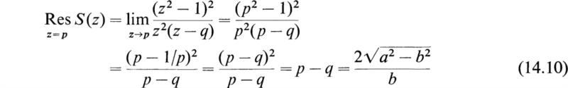
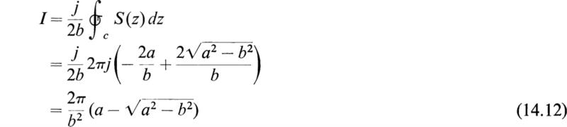
As an example of the general procedure, let it be required to prove that if a > b > 0
If we let ejθ = z, this becomes
where
These are the two roots of the quadratic
It is seen that p is the only simple pole of the integrand inside the unit circle c, and the origin is a pole of order 2. We must now compute the residues of
at the poles z = p and z = 0.
We do this by the methods of Sec. 12. The residue at z=p may be evaluated by formula (12.2). We thus obtain
The residue at the double pole z = 0 may be evaluated by Eq. (12.12); it is
Now, by Cauchy’s residue theorem (9.11), we have
This prove the result.
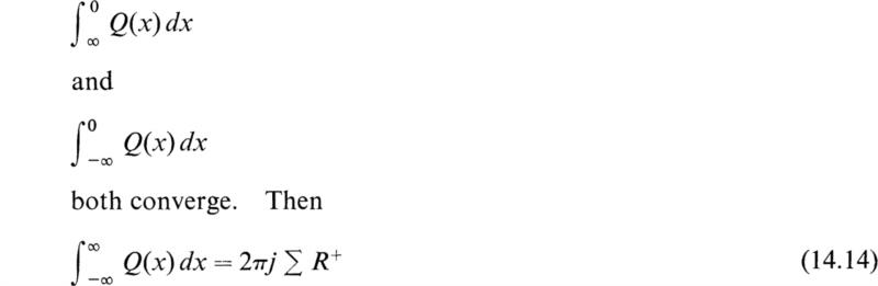
We shall now consider the evaluation of integrals of the type
where Q(z) is a function that satisfies the following restrictions:
1. It is analytic in the upper half plane except at a finite number of poles.
2. It has no poles on the real axis.
3. zQ(z) →0 uniformly as |z| → ∞ for ![]()
4. When x is real, xQ(x) → 0 as x → ±∞ in such a way that
where ∑ R+ denotes the sum of the residues of Q(z) at its poles in the upper half plane.
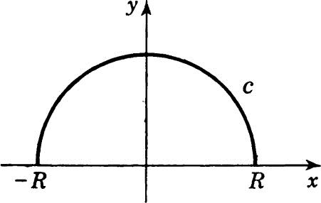
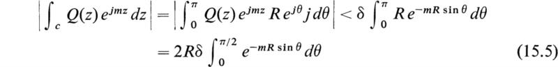
To prove this, choose as a contour a semicircle c with center at the origin and radius R in the upper half plane, as shown in Fig. 14.1. Then, by Cauchy’s residue theorem, we have
Now by condition 3, if R is large enough, we have
for all points on c, and so
Fig. 14.1
Hence as R → ∞, the integral around c tends to zero, and if (4) is satisfied, we have Eq. (14.14).
This theorem is particularly useful in the case when Q(x) is a rational function. As an example of this theorem, let it be required to prove that if a > 0
Consider
This function has simple poles at aeπj/4, ae3πj/4, ae5πj/4, ae7πj/4. Only the first two of these poles are in the upper half plane. The function Q(z) clearly satisfies the conditions of the theorem; therefore
By the methods of sec 12, we have
Hence
and
Therefore
Since the function Q(x) is an even function of x, we have
Hence
A very useful and important theorem will now be proved. It is usually known as Jordan’s lemma.
Let Q(z) be a function of the complex variable z that satisfies the following conditions:
1. It is analytic in the upper half plane except at a finite number of poles.
2. Q(z) → 0 uniformly as |z| → ∞ for 0 < arg z < π.
3. m is a positive number.
Then
where c is a semicircle with its center at the origin and radius R.
Proof. For all points on c we have
Now
By condition 2, if R is sufficiently large, we have for all points on c
Hence
It can be proved that sin θ/θ decreases steadily from 1 to 2/π as θ increases from 0 to π/2. Hence
Therefore
from which (15.1) follows.
By the use of Jordan’s lemma the following type of integrals may be evaluated: Let
where N(z) and D(z) are polynomials and D(z) has no real zeros. Then if (i) the degree of D(z) exceeds that of N(z) by at least 1, and (ii) m > 0, we have
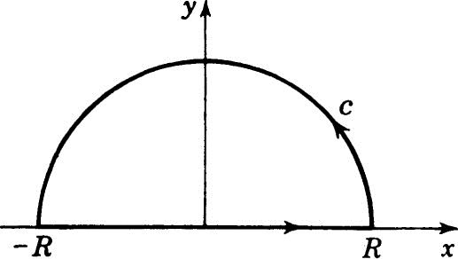
where ∑ R+ denotes the sum of the residues of Q(z)ejmz at its poles in the upper half plane. To prove this, integrate Q(z)ejmz around the closed contour of Fig. 15.1. We then have
Since Q(z)ejmz satisfies the conditions of Jordan’s lemma, we have on letting R →∞ the result (15.9) since the integral around the infinite semicircle vanishes. Taking the real and imaginary parts of (15.9), we can evaluate integrals of the type
As an example, let it be required to show that
Here we consider the function ejz/(z2 + a2), and since it satisfies the above conditions, we have
The only pole of the integrand in the upper half plane is at ja; the residue there is e–a/2ja. Hence
Fig. 15.1
Therefore, taking the real part of ejx, we have
Hence (15.12) follows.
By an extension of the above theorem it may be proved that
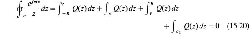
To prove this, let us consider the integral
taken about the contour of Fig. 15.2, where c1 is a semicircle of radius R and s is a semicircle of radius r.
We notice that the integrand
has a simple pole at z = 0 and none in the upper half plane. By Jordan’s lemma, we have
where c1 is a semicircle of radius R and center at the origin. Since the contour c does not enclose any singularities of the integrand, we have by Cauchy’s residue theorem
Fig. 15.2
Now, on the semicircle s, we have †
and
Letting R → ∞ and r → 0 in (15.20), we have
On equating real and imaginary parts we get
Hence, since the integrand of the second integral is an even function of x, we have
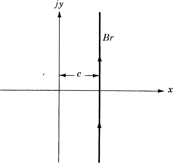
A particular type of contour integral that occurs with great frequency in mathematical analysis is the Bromwich contour integral, which is illustrated in Fig. 16.1. This contour extends from c – j∞ to c + j∞ where ![]() A typical integral involving the Bromwich integral is of the form
A typical integral involving the Bromwich integral is of the form
Fig. 16.1
Fig. 16.2
which is known as the inversion formula for Laplace transforms. The function f(t) is said to be the inverse Laplace transform of the function g(z).† The constant c is adjusted such that all of the singularities of g(z) lie to the left of the Bromwich contour. This requirement is necessary for the integral to exist.
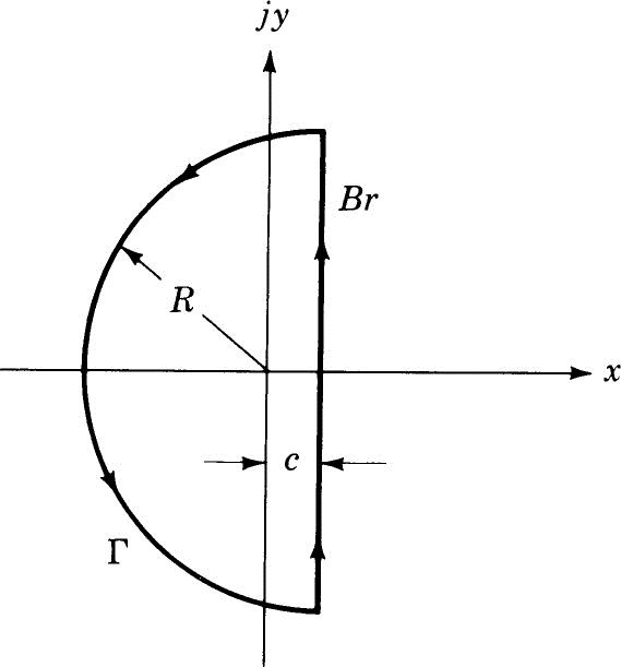
The evaluation of any integral involving the contour indicated by Eq. (16.1) is accomplished in the same manner as discussed in the previous sections. In most cases the Bromwich contour is closed by adding a semicircular path Γ on the left, as illustrated in Fig. 16.2. Jordan’s lemma can be applied in this case to obtain conditions on g(z) such that
and hence by Cauchy’s residue theorem
Comparing this expression with (16.1) leads to the result that
To illustrate the procedure we shall find f(t) corresponding to the complex function g(z) = 1/(z + a), where a is a real positive constant. From (16.1) we have
By (16.4) we may see that f(t) = ∑ Res in (Br +Γ) since it may be easily shown that the contribution of ezt/(z + a) around Γ vanishes as R → ∞ provided c = 0. The setting of c to zero does not affect the problem since in moving the contour Br to coincide with the imaginary axis no singularities of g(z) were crossed.
The only singularity of g(z) occurs at z = – a; therefore, according to Sec. 12, the residue is
Thus, the solution of (16.5) is
As a second example consider the function
Again it may be easily verified that g(z) satisfies the conditions of Jordan’s lemma, and hence it may be stated that
or by (16.4)
By inspection of (16.7) it is easily seen that g(z) has two double poles, one at z = jw and the other at z = –jw. Since these poles lie on the imaginary axis, the positive constant c in the Bromwich contour integral must be chosen such that c > 0, or else the contour will cross the singularities.
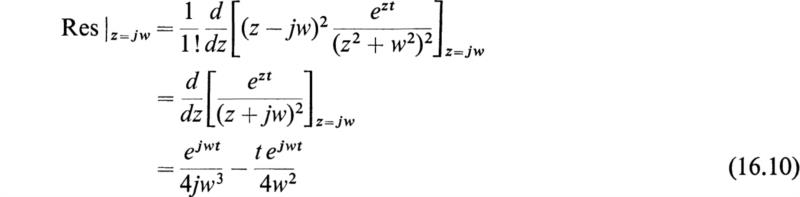
All that remains now is to evaluate the residues of ezt/(z2 + w2)2 at the two double poles. To do this we shall employ the residue formula given by (12.13). For the double pole at z = jw we have
To evaluate the residue at z = –jw, simply take the complex conjugate of (16.10); that is, set j = –j. Performing this operation yields
Adding the results of (16.10) and (16.11) gives the sum of both residues and hence by (16.9)
This expression is easily reduced by applying the Euler formulas (2.9). The final result is
Frequently integrals of the following type are encountered:
where a is not an integer. These integrals may be evaluated by contour integration; however, since za–1 is a multiple-valued function, it is necessary to introduce a barrier or cut in the z plane. The reason for this may be illustrated in the following manner.
As seen in Sec. 5, any contour integral over a closed contour containing a finite number of singularities may be reduced to a series of closed contour integrals, one around each singularity. Hence no loss in generality will occur if we consider a contour integral about the origin containing a single singular point at the origin, viz.,
where C is a closed contour enclosing the origin.
Now let us examine the function w(z) = z–b which comprises the integrand of (17.2). If z = rejθ, then it is easy to see that
Hence, if a point on the contour C makes one complete circuit of the origin, then the change in the argument of w(z) is
Now if b is an integer, then w(z) returns to the same value it had prior to circumnavigating the origin. However, if b is not an integer, then w(z) does not return to its original value.
If ![]() then two complete circuits of the origin would be required in order to return w(z) to its initial value. Because of this peculiarity, the function w(z) is said to have a branch point at the origin. The function w(z) is said to have as many branches as the number of complete circuits around the branch point required to return the function to its original value. The number of branches may also be easily identified from b because if b is of the form 1/n, where n is an integer, then the function w(z) has n branches. In the example the function
then two complete circuits of the origin would be required in order to return w(z) to its initial value. Because of this peculiarity, the function w(z) is said to have a branch point at the origin. The function w(z) is said to have as many branches as the number of complete circuits around the branch point required to return the function to its original value. The number of branches may also be easily identified from b because if b is of the form 1/n, where n is an integer, then the function w(z) has n branches. In the example the function ![]() has two branches, one corresponding to
has two branches, one corresponding to ![]() and the other to
and the other to ![]() .
.
In order to avoid the problem of determining which branch the function is on when performing a contour integration about the origin, a branch cut is introduced into the complex z plane. This cut restricts the argument of w(z) to a range of only 2π. This is accomplished by simply following the rule that once a branch cut has been introduced into the z plane, any contour of integration may not cross it. This artifice of an impassable cut in the z plane automatically restricts w(z) to remain on only one of its branches.
Branch cuts always start at the branch point and terminate either at infinity or at another branch point.†
Returning to our original problem, Eq. (17.1), one method of evaluating integrals of this type is to use a contour consisting of a large circle C with center at the origin and radius R. The plane must be cut along the real axis from 0 to ∞ and the branch point at z = 0 enclosed by a small circle s of radius r, as shown in Fig. 17.1.
Now let Q(x) be a rational function of x with no poles on the positive real axis. Let us write
Fig. 17.1
and
We then get the integral around C tending to zero as R →∞ and the integral around s tending to zero as r → 0. Hence, on making R → ∞ and r → 0, we get
where ∑ R is the sum of the residues of w(z) inside the contour. It must be noticed that the values of xa–1 at points on the upper and lower sides of the cut are not the same. This may be seen as follows.
If z = rejθ, we have
and the values on the upper side of the cut correspond to |z| = x and θ = 0, and at the lower side they correspond to |z| =x and θ = 2π. Since
we get
As an example of this method of integration, let us evaluate the integral
This integral is of importance in the theory of gamma functions discussed in Appendix B, Sec. 27.
In this case we have
Hence, if 0 < a < 1, conditions (17.6) and (17.7) are satisfied. w(z) has a pole at z = – 1. The residue at z = – 1 is
Hence, by (17.11), we have
In this section we shall consider two more examples of Bromwich contour integrals of functions containing branch points.
The first example is a contour integral which is of importance in solving problems in heat conduction.
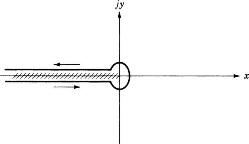
The integrand of (18.1) has a branch point at the origin. Because there are no other singularities in the z plane, the Bromwich contour may be deformed into the one shown in Fig. 18.1, in which the arrows indicate the direction of integration.
It will be convenient to break the integration into three parts:
I1 = the contour below the branch cut on which z = re–jπ
I2 = the contour around the small circle at the origin on which z = ![]() ejθ
ejθ
I3 = the contour above the branch cut on which z = rejπ
Thus we may write
Fig. 18.1
Examining I2, the limit and integral may be interchanged. Performing this and the indicated operations yields the result ![]() Since I1 and I3 involve
Since I1 and I3 involve ![]() only in the limits of integration,
only in the limits of integration, ![]() may be set directly to 0 and (18.2) and (18.4) combined to give
may be set directly to 0 and (18.2) and (18.4) combined to give
Expanding the sine function in a Taylor’s series

and integrating (18.6) term by term results in
where ![]()
The series in (18.7) is an expansion of the function known as the error function, that is, ![]() which permits (18.7) to be expressed in the following form:
which permits (18.7) to be expressed in the following form:
Combining all the components of the integral given in (18.1) and represented by (18.5) yields†
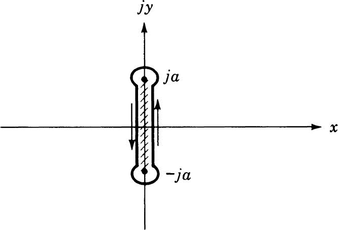
Our second example involves two branch points that are located at z = ±ja. In this example we have
To evaluate this integral the Bromwich contour will be deformed into the dumbbell contour shown in Fig. 18.2. A branch cut is introduced between
Fig. 18.2
z = ±ja since the integrand has two branch points, one at each of the designated points.
The evaluation of f(t) is accomplished by breaking the integral into four parts:
If we now take the limit ![]() → 0 we find I2 and I4 both vanish. This leaves us with the result
→ 0 we find I2 and I4 both vanish. This leaves us with the result
This latter expression may be reduced to
To evaluate (18.13) we introduce the transformation y = a sin θ and we find the following integral:
This expression is a standard form for the representation of the Bessel function of the zeroth order, that is,
At various times in mathematical analysis it becomes convenient to make use of many of the properties of complex conjugates; it is the purpose of this section to introduce a few of the interesting properties that result from the study of conjugates. It is well known that the complex variable z and its conjugate are defined by
Now if we consider a function ø which is a function of z and ![]() that is,
that is, ![]() its derivatives with respect to x and y are
its derivatives with respect to x and y are
Now defining the operators
we may rewrite Eqs. (19.2) and (19.3) as
or
From (19.7) we may readily obtain
Hence we see that the Laplace operator may be expressed in the form
The expression of the Laplacian operator in the form of (19.9) allows us to obtain a class of solutions quite easily. Using the notation introduced, Laplace’s equation becomes
which implies that Laplace’s equation may be written as
To obtain a solution to this equation we need only to integrate with respect to z first and then z as follows:

or
This equation is known in classical literature as D’Alembert’s solution.
As a second topic let us consider Green’s theorem in two dimensions, which, from Appendix E, is
Using our notation, we have
If we now consider the double integral
But from (19.13) we have
If we now let Q = F and –P = jF, then (19.16) becomes
However,

and
![]()
Therefore (19.17) may be written in the form

or
which is known as the complex form of Green’s theorem.
As examples of the application of the complex form of Green’s theorem, we may consider the evaluation of area integrals. To accomplish this let

Then (19.18) becomes
and since
![]()
we find that
As a specific example, consider a circle defined by z = rejθ. We thus have the relations
![]()
from which we quickly find that

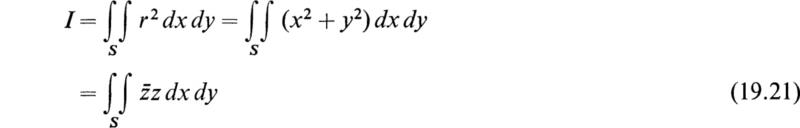
Another application of the complex form of Green’s theorem is the computation of moments of inertia of plane areas about the origin, or the polar moments of inertia. Consider an area S in the xy plane bounded by a simply connected contour C. By definition the polar moment of inertia is given by
However, from (19.18) we have
To apply (19.22) let
Substituting into (19.22) yields the complex form for the polar moment of inertia.
Complex notation is also convenient for deriving Cauchy’s integral theorem. Let us again consider Eq. (19.18):
If we let F = w, we have
Now if ![]() inside and on C we have
inside and on C we have
![]()
But
However,

and hence
which are the Cauchy-Riemann equations. This implies that the condition ![]() is the same as the Cauchy-Riemann equations and hence w is analytic whenever this condition is fulfilled. Thus if w is analytic then
is the same as the Cauchy-Riemann equations and hence w is analytic whenever this condition is fulfilled. Thus if w is analytic then ![]() and by (19.26)
and by (19.26)
which is Cauchy’s integral theorem.
Morera’s theorem, which states that if (19.29) is true then ![]() and w is analytic also follows easily from the complex form of Green’s theorem.
and w is analytic also follows easily from the complex form of Green’s theorem.
Other interesting items using the complex conjugate notation are the relations between u(x,y), v(x,y), and w(z). To develop these relations let us consider
If we let y = 0, then
Placing x = z in (19.31) yields
Equation (19.32) states that the functional form of w(z) may be formulated directly from u(x,y) and v(x,y). As an example, let us consider the functions
Setting y = 0 gives
![]()
and hence from (19.32) we have
The above result may easily be verified.
As a final item we will derive a method using the properties of complex conjugates for determining w(z) when either u(x,y) or v(x,y) are given. First let us consider the case when u(x,y) is known and it is desired to determine w(z). We have
![]()
hence
or
by making use of the Cauchy-Riemann relation. Now if we place y = 0 in (19.36)
![]()
Setting x = z in this relation yields
![]()
and therefore
In a similar fashion if v(x,y) is known, then we may derive the relation
As an example let us consider the problem where
![]()
Now
![]()
and hence
![]()
From (19.37) we have
As a further example consider
![]()
from which
![]()
and from (19.38)
1. Show that the function w(z) = |z|2 has a unique derivative at the origin but nowhere else.
2. Show that the real and imaginary parts of sin z satisfy Laplace’s equation in two dimensions.
3. Find the residues of w(z) = ez/(z2 + a2) at its poles.
4. Find the poles of the function w(z) = ez/sinz.
5. Find the sum of the residues of the function w(z) = ez/(z cosh mz) at its poles.
6. Prove that

7. Prove that

HINT: Integrate eaz/sinh πz around the rectangle of sides y = 0, y = 1,x = ±R, indented at the origin and at j.
8. Show that, if m and n are positive integers and m<n,

9. Show that, if m > 0, a > 0,


HINT: Integrate ejz/(z – ja) over a suitable contour.

13. Show that, if -π < a < π,

HINT: Integrate eaz/cosh πz around the rectangle of sides x = ±R, y = 0, y = 1.

15. By integrating ![]() around a suitable contour show that
around a suitable contour show that

16. By integrating ![]() along a suitable path show that
along a suitable path show that

17. By taking as a contour a square whose corners are ±N, ±N+ 2Nj, where N is an integer, and letting N →∞, prove that


22. Compute the first terms of ![]() i, i= 1, 2, 3, 4, in (3.9).
i, i= 1, 2, 3, 4, in (3.9).
23. Derive (3.11).
24. Find u(x,y) and v(x,y)for (a) w = z2; (b) w = ez; (c) w = 1/z; (d) w = cosz; and (e) w = sinhz.
25. Given u(x,y) = –cosx sinh y, find u(x,y) and w(z).
26. Given u(x,y) = ln ![]() , find v(x,y) and w(z).
, find v(x,y) and w(z).
27. Rewrite (7.7) and (7.8) to represent a Taylor’s series expansion about the origin.
28. Show that (7.6) is correct.
29. Show that the expansion of (8.15) is correct by applying (8.6) and (8.7) to the first few terms.
30. Derive (9.3) by integrating (9.2) around a unit circle centered at z = z0.
HINT: Show that the only nonzero contribution of this integration is the result given by Eq.(9.3).
31. Rewrite the conditions in Jordan’s lemma to apply to g(z) in (16.2).
32. Derive the solution given by (16.14) by shrinking the contour (Br + Γ) to unit circles around each of the singularities and performing each of the integrations.
33. Evaluate

34. Evaluate each of the following integrals by enclosing all the singularities in the finite plane with a closed contour (the constants a and b may be real or complex) :

(McLachlan, 1955, p. 320)

for ![]()
36. Derive Eqs. (6.13) and (6.14) by the method stated.
37. Verify Eq. (8.9).
38. Equation (8.12) yields an expansion of 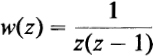 about the origin which is valid in the interval 0 < z < 1. Obtain an expansion for w(z) about z = 0 that is valid in the interval z > 1.
39. Compute the polar moment of inertia of a circle of radius a about the origin.
40. Compute the polar moment of inertia of a square centered at the origin and side a.
41. Derive a formula for the moment of inertia of a plane area about the y axis in complex form:

42. Derive (19.38).
43. Given u(x,y) = ex cos y, find w(z) by the complex conjugate method.
![]()
find w(z) by the complex conjugate method.
45. Evaluate the contour integral

1927. Whittaker, E. T., and G. N. Watson: “A Course in Modern Analysis,” Cambridge University Press, New York.
1933. MacRobert, T. M.: “Functions of a Complex Variable,” The Macmillan Company, New York.
1933. Rothe, R., F. Ollendorf, and K. Pohlhausen: “Theory of Functions as Applied to Engineering Problems,” M.I.T. Press, Cambridge, Mass.
1955. McLachlan, N. W.: “Complex Variable and Operational Calculus,” Cambridge University Press, New York.
1958. Pipes, L. A.: “Applied Mathematics for Engineers and Physicists,” McGraw-Hill Book Company, New York.
† Readers who would like a brief review of complex numbers are referred to Pipes, 1958, chap. 2 (see References at the end of this chapter).
† H. Nyquist, Regeneration Theory, Bell System Technical Journal, p. 126, January, 1932.
† A very useful fact to remember is that an integral over a small semicircular contour centered at a simple pole is always equal to half the residue of the simple pole.
† In standard transform literature the complex variable z is replaced by s.
† See McLachlan, 1955, p. 70 ff., for several examples of branch cuts (see References).
† The notation erfc denotes the complementary error function which is defined in terms of erf as in (18.8) above. The function erf x has the following integral representation: