The equations of applied mathematics express relations between quantities that are capable of measurement in terms of certain defined units. The simplest types of physical quantities are completely defined by a certain simple number. Examples of such quantities are mass, temperature, length. Such quantities are called scalars.
There are, however, other physical quantities that are not scalars. Such quantities as the displacement of a point, the velocity of a particle, a mechanical force require three numbers to specify them completely. The three numbers that are required to specify the quantities are scalars and could be, for example, the components of the displacement of the particle with respect to an arbitrary cartesian coordinate reference frame.
We could carry out the various mathematical operations with these scalar quantities, but we would be neglecting the fact that from a physical point of view a displacement, for example, is one entity, and also we are introducing a foreign element into the question, that is, the coordinate system.
Accordingly it has been found convenient to introduce a mathematical discipline that enables us to study quantities of this type without recourse to a definite coordinate system.
It is only when we come to evaluate formulas numerically that it will be necessary to introduce a definite coordinate system. The mathematical technique that enables us to do this is vector analysis.
A physical quantity possessing both magnitude (length) and direction is called a vector. Typical examples are force, velocity, acceleration, momentum. It is customary to represent vectors by letters in boldface type and scalars in lightface italics.
A vector may be indicated graphically by an arrow drawn between two points. It is thus evident that rectilinear displacements of a point and all physical quantities that can be represented by such displacements in the same manner that a scalar can be represented by the points of a straight line are vectors.
A vector having been defined as an entity that behaves in the same manner as the rectilinear displacement of a point, vector addition is reduced to a composition of linear displacements.
Consider two vectors A and B, as shown in Fig. 3.1. The vector C, which is obtained by moving a point along A and then along B, is called the resultant, or sum, of the vectors A and B, and we write
From the nature of the definition of vector addition it is apparent that
and that therefore vector addition is commutative. If the vectors A and B are situated as shown in Fig. 3.2, then the resultant vector C is obtained by completing the parallelogram formed by the two vectors.
Fig. 3.1
Fig. 3.2
In general, the sum of the vectors A and B is obtained by placing the origin of B at the terminus of A. Then the vector C extending from the origin of A to the terminus of B is defined as the sum, or resultant, of A and B.
To add several vectors A, B, and C, first find the sum of A and B and the sum of A + B and C. It is seen that the result is the same as finding the sum of B and C first and then the sum of A and B + C. Thus vector addition is associative.
![]()
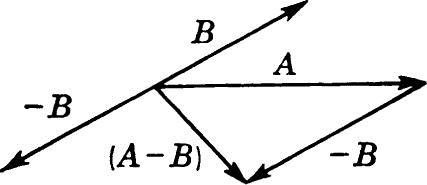
To subtract B from A, add –B to A, as shown in Fig. 3.3.
Two vectors are said to be equal if they have the same magnitude and the same direction.
By the product of a vector a by a scalar n we understand a vector whose magnitude is equal to the magnitude of the product of the magnitudes of a and n and has the same direction as a or the opposite direction, depending on whether the scalar n is positive or negative. We thus write
to denote this new vector.
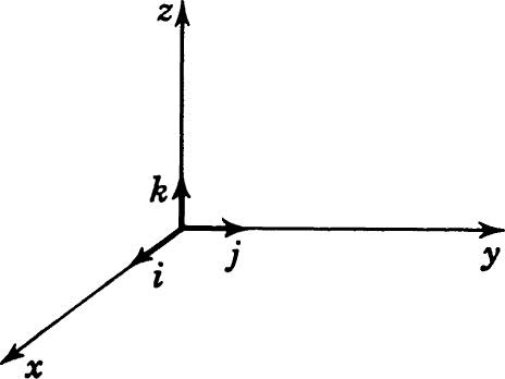
A vector having unit magnitude is called a unit vector. The most common unit vectors are those which have the directions of a right-handed cartesian coordinate system as shown in Fig. 3.4. The vector i is a unit vector having the x direction of the coordinate system; the unit vector j has the y direction; and the unit vector k has the z direction.
The components of a vector A are any vectors whose sum is A. The components most frequently used are those parallel to the axes x, y, and z. These
Fig. 3.3
Fig. 3.4
are called the rectangular components of the vector. If Ax, Ay, and Az are the projections of A on the axes x, y, z, respectively, we may write
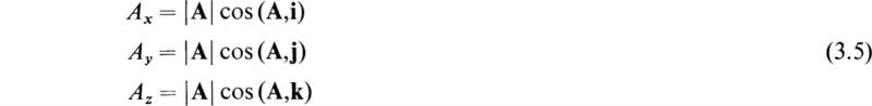
If a vector A is given in magnitude and direction, then its components along the three axes of a cartesian reference frame are given by
where |A| denotes the magnitude of the vector. If, conversely, the three components of the vector are assigned, the vector A is uniquely specified as the diagonal of the rectangular parallelepiped whose edges are the vectors iAx, jAy and kAz. Its magnitude is
and its direction is given by the three cosines which can be found from (3.5) and (3.6).
The scalar, or dot, product of two vectors is defined as a scalar quantity equal in magnitude to the product of the magnitudes of the two given vectors and the cosine of the angle between them. The scalar product of the two vectors A and B is thus given by the equation
The cosine of the angle between the directions of the two vectors becomes +1 when the directions are the same, –1 when they are opposite, and 0 when they are perpendicular.
It is clear from the definition of the dot product that the commutative law of multiplication holds, that is,
The fact that the distributive law of multiplication holds can be seen with the aid of Fig. 4.1. We have from the figure
From the fundamental unit vectors we can form the following scalar products:
Fig. 4.1
As a consequence of these results, we obtain
We may also write
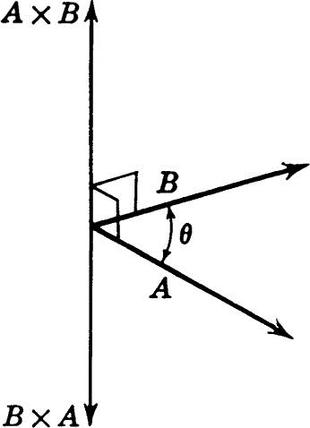
The vector, or cross, product of two vectors is defined to be a vector perpendicular to the plane of the two given vectors in the sense of advance of a right-handed screw rotated from the first to the second of the given vectors through the smaller angle between their positive directions.
The meaning of this definition is made clear in Fig. 5.1. The magnitude of this vector is equal to the product of the magnitudes of the two given vectors times the sine of the angle between them.
The vector, or cross, product is denoted by A × B. As is clear from the definition and the figure, the commutative law does not hold for this type of multiplication; instead we have
Also we have
It follows from the definition that if the vector product of two vectors vanishes, the vectors are parallel provided neither vector is zero.
Fig. 5.1
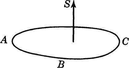
Let us consider a plane surface such as shown in Fig. 5.2. Since this surface has a magnitude represented by its area and a direction specified by its normal, it is a vector quantity. A certain ambiguity exists as to the positive sense of the normal. In order to remove this ambiguity, the following conventions are adopted:
If the surface is part of a closed surface, the outward-drawn normal is taken as positive.
If the surface is not part of a closed surface, the positive sense in describing the periphery is connected with the positive direction of the normal by the rule that a right-handed screw rotated in the plane of the surface in the positive sense of describing the periphery advances along the positive normal. For example, in Fig. 5.2, if the periphery of the surface is described in the sense ABC, the positive sense of the normal, and therefore the direction of the vector S representing the surface, is upward.
If a surface is not plane, it may be divided into a number of elementary surfaces each of which is plane to any desired degree of approximation. In this case the vector representative of the entire surface is the sum of the vectors representing its elements. Two surfaces, considered as vectors, are equal if the representative vectors are equal. Therefore two plane surfaces are equal if they have equal areas and are normal in the same direction even if they have different shapes.
A curved surface may be replaced by a plane surface perpendicular to its representative vector having an area equal to the magnitude of this vector. The vector representing a closed surface is zero because the projection of the entire surface on any plane is zero; since as much of the projected area is negative as positive, it therefore follows that the vector representing the entire surface has zero components along the three axes x, y, z, and consequently it equals zero.
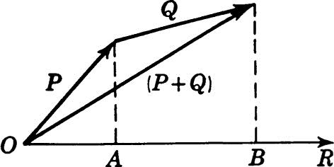
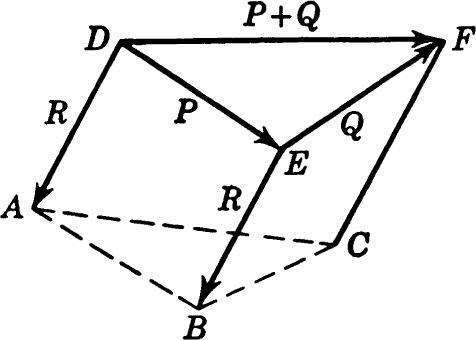
To prove that the distributive law of multiplication holds for the vector product, consider the prism of Fig. 5.3. The edges of this prism are the vectors P, Q,
Fig. 5.2
Fig. 5.3
P + Q, and R. The vectors representing the faces of the closed prism are
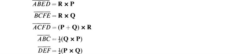
Therefore the representative vector for the entire polyhedral surface is
or
By the definition of the vector product we have the following relations for the unit vectors:
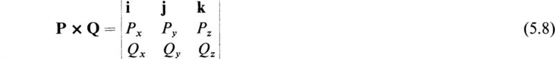
If we write the vectors P and Q in terms of their rectangular components,
and realize that the distributive law holds for a vector product, we obtain
in view of the properties of the unit vectors expressed by (5.5). This expression can be represented in a compact fashion by the determinant
There are several types of multiple products used in vector analysis, and in this section the most important types will be considered.
Here B·C is a scalar so that A(B·C) is a vector parallel to A and is of course an entirely different vector from (A·B)C.
Consider A·B × C. In this case we have the important relation
The proof of this relation follows from the fact that each of these expressions represents the volume of the parallelepiped whose edges are A, B, C. Furthermore, all three expressions give this volume with the positive sign provided the vectors A, B, C, in that order, form a right-handed system.
Consider the product
By the definition of a cross product q is perpendicular to the vector a and also to the vector b × c. Accordingly the vector q lies in the plane of b and c and may be expressed in the form
where u and υ are scalar multipliers.
Now we have
or
Hence
Now let
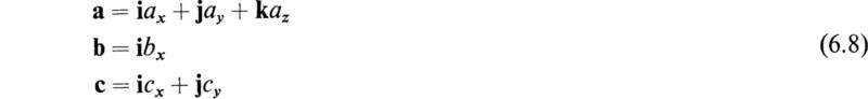
where n is some scalar. To find the magnitude of n, consider a set of cartesian coordinate axes oriented so that the vectors a, b, and c have the following components in terms of these axes:
Hence, comparing (6.9) and (6.10), it is seen that the constant n is equal to 1.
The differential coefficient or derivative of a vector A with respect to a scalar variable t, say, the time, is defined as a limit by the equation
Since division by a scalar does not alter vectorial properties, the derivative of a vector with respect to a scalar variable is itself a vector.
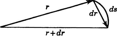
As an example of differentiation of a vector with respect to a scalar, consider a particle p moving along a curve c, as shown in Fig. 7.1. Let the position of the particle with respect to the origin of a cartesian reference frame be denoted by r. In that case the velocity of the particle is given by
where ds is a differential of arc measured along the curve, as shown in Fig. 7.2. Now
Fig. 7.1
Fig. 7.2
where T is a unit vector tangent to the curve defining the path of the particle. Hence we have
The quantity ds/dt is the speed of the particle. The acceleration of the particle is defined as the time derivative of the velocity. We thus have
Now
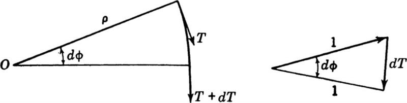
Consider Fig. 7.3.
We may write
Substituting these expressions into (7.6), we obtain
Substituting this into (7.5), we finally obtain
We thus see that the acceleration of the particle consists of two terms. The first term depends upon the rate of change of speed of the particle and is directed along the tangent to the particle; the second term is the centripetal
Fig. 7.3
acceleration of the particle and depends on the radius of curvature ρ of the particle and the square of the speed. This acceleration is directed in a direction normal to the curve and toward the center of curvature.
Since the derivatives of vectors with respect to a scalar variable are deduced by a limiting process from subtraction of vectors and division by scalars, which are operations subject to the rules of ordinary algebra, it follows that the rules of the differential calculus can be extended at once to the differentiation of a sum of vectors,
or the product of a scalar and a vector,
And, similarly,
An interesting application of vector differentiation of importance to mechanics will now be discussed. Consider a small insect on a rotating plane sheet of cardboard. The cardboard will be assumed to be rotating about a fixed point O with a uniform angular evlocity w. It will be supposed that the insect may move with respect to the cardboard. In order to describe the velocity and acceleration of the moving insect, let a cartesian coordinate system x, y be drawn on the rotating cardboard with the center of rotation as the origin. Let the position vector of the insect be
where i and j are unit vectors in the x and y directions that rotate with the cardboard. The velocity of the insect v relative to fixed space is
Now, since i and j are unit vectors rotating with angular velocity w, it is easy to show by the reasoning of Eqs. (7.6) and (7.10) that
Hence (7.17) may be written in the form
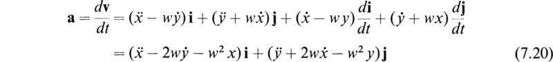
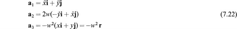
where the dots indicate differentiation with respect to the time in the usual manner. The acceleration a of the insect is given by
Equation (7.20) indicates that the acceleration of the insect consists of three separate terms of the form
where
a1 is the acceleration of the insect with respect to the rotating coordinate system. If the angular velocity w were zero and the card were stationary, this would be the only acceleration. a2 is the so-called Coriolis’ acceleration. It depends on the angular velocity w of the rotating card and on the velocity of the particle relative to the rotating coordinate axis. This relative velocity vr is given by
If the scalar product of the relative velocity vr and the Coriolis’ acceleration a2 is taken, the following result is obtained:
This indicates that the Coriolis’ acceleration is perpendicular to the relative velocity.
The acceleration a3 is the centripetal acceleration. Its magnitude is proportional to the square of the angular velocity w of the frame of reference and to the distance of the particle from the center of rotation. It is directed radially toward the center of rotation. Equation (7.20) may be generalized, and the acceleration of a particle in a rotating reference plane such as the earth can be computed. The Coriolis’ acceleration causes deviation of falling bodies and projectiles and explains the motion of Foucault’s pendulum.†
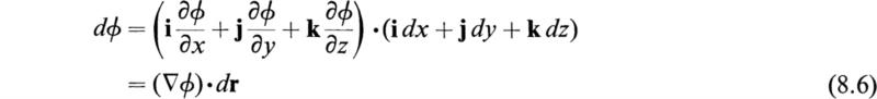
Let ϕ(x,y,z) be a scalar function of position in space, that is, of the coordinates x, y, z. If the coordinates x, y, z are increased by dx, dy, dz, respectively, we have
If we denote by dr the vector representing the displacement specified by dx, dy, dz, then
In vector analysis a certain vector differential operator ∇ (read “del”) defined by
plays a very prominent role. The gradient of a scalar function ϕ(x,y,z) is defined by
Operating with ∇ on the scalar function ϕ(x,y,z), we get
This is just the expression (8.4) defined as the gradient of ϕ. Now, from (8.1) and (8.2), we have
The equation
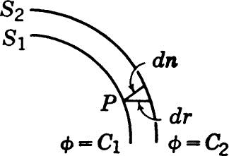
represents a certain surface, and as we change the value of the constant, we obtain a family of surfaces.
Consider the surfaces of Fig. 8.1. If dn denotes the distance along the normal from the point P to the surface S2, we may write
where n is the unit normal to the surface S1 at P. We have
Fig. 8.1
and, in particular, if dr lies in the surface S1 we have
showing that the vector ∇ϕ is normal to the surface ϕ = const. Since the vector dr is arbitrary, we have from (8.9)
Hence ∇ϕ is a vector whose magnitude is equal to the maximum rate of change of ϕ with respect to the space variables and has the direction of that change.
The scalar product of the vector operator ∇ and a vector A gives a scalar that is called the divergence of A; that is,
This quantity has an important application in hydrodynamics.
Consider a fluid of density ρ(x,y,z,t) and velocity v = v(x,y,z,t), and let
If S is the representative vector of the area of a plane surface, then V·S is the mass of fluid flowing through the surface S in a unit time.
Consider a small fixed rectangular parallelepiped of dimensions dx, dy, dz, as shown in Fig. 9.1. The mass of fluid flowing in through face F1 per unit time is
and that flowing out through face F2 is
Hence the net increase of mass of fluid inside the parallelepiped per unit time is
Fig. 9.1
Considering the net increase of mass of fluid per unit time entering through the other two pairs of faces, we obtain
as the total increase in mass in the parallelepiped per unit time.
But by the principle of conservation of matter, this must be equal to the time rate of increase of density multiplied by the volume of the parallelepiped. Hence
or
This is known in hydrodynamics as the equation of continuity. If the fluid is incompressible, then
The name divergence originated in this interpretation of ∇·V. For since – ∇·V represents the excess of the inward over the outward flow, or the convergence of the fluid, so ∇·V represents the excess of the outward over the inward flow, or the divergence of the fluid.
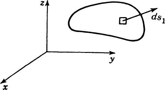
Consider a surface s as shown in Fig. 9.2. Divide the surface into the representative vectors ds1, ds2, . . . , etc. Let Vi be the value of the vector function of position Vi(x,y,z) at dsi. Then
Fig. 9.2
is known as the surface integral of V over the surface s. The sign of the integral depends on which face of the surface is taken as positive. If the surface is closed, the outward normal is taken as positive.
Since
we have
The surface integral of a vector V is called the flux of V throughout the surface.
This is one of the most important theorems of vector analysis. It states that the volume integral of the divergence of a vector field A taken over any volume V is equal to the surface integral of A taken over the closed surface surrounding the volume V; that is,
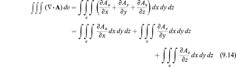
To prove Gauss’s theorem, let us expand the left-hand side of Eq. (9.13). We then have
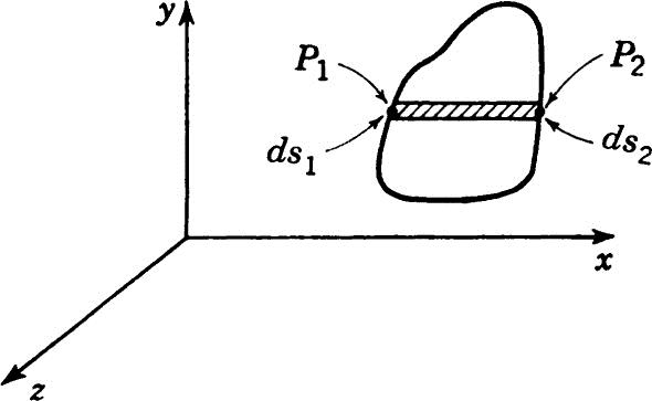
Let us consider the first integral on the right. Integrate with respect to x, that is, along a strip of cross section dydz extending from P1 to P2 of Fig. 9.3. We thus obtain
Fig. 9.3
Here (x1, y, z) are the coordinates of P1 and (x2y,z) are the coordinates of P2. Now at P1 we have
At P2 we have
Therefore
where the surface integral on the right is evaluated over the entire surface. In the same manner we obtain
If we now add (9.18), (9.19), and (9.20), we obtain Gauss’s theorem:
By the use of Gauss’s theorem we are able to make some important transformations. Consider
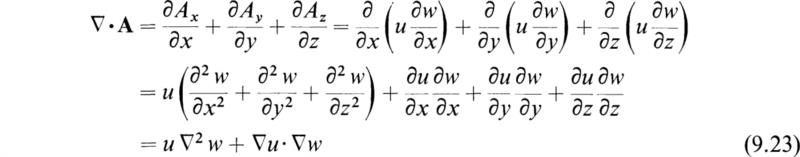
that is, let the vector field A be the product of a scalar function u and the gradient of another scalar function w. Consider
If we place this value of ∇·A in the left-hand side of Gauss’s theorem (9.21), we obtain
This transformation is referred to as the first form of Green’s theorem.
In (9.24) if we interchange the functions u and w, we obtain
If we now subtract Eq. (9.25) from Eq. (9.24), we obtain
This transformation is referred to as the second form of Green’s theorem. The transformations (9.24) and (9.26) are of extreme importance in the fields of electrodynamics and hydrodynamics.
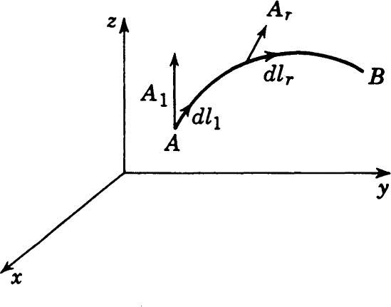
Let A be a vector field in space and AB (Fig. 10.1) a curve described in the sense A to B. Let the continuous curve AB be subdivided into infinitesimal vector elements dI1, dI2,. . . , dIn. Take the scalar products A1·dI1,
Fig. 10.1
A2·dI2, . . . , An·dIn, where A1, A2, . . . , An are the values that the vector field A takes at the junction points of the vectors dI1, dI2, . . . , dIn. The sum of these scalar products, that is,
summed up along the entire length of the curve, is known as the line integral of A along the curve AB. It is obvious that the line integral from B to A is the negative of that from A to B.
In terms of cartesian components we can write
If F represents the force on a moving particle, then the line integral of F over the path described by the particle is the work done by the force.
Let A be the gradient ∇ϕ of a scalar function of position; that is,
Then
But we have
the total differential of ϕ. We thus have
where ϕB and ϕA are the values of ϕ at the points B and A, respectively. It follows from this that the line integral of the gradient of any scalar function of position ϕ around a closed curve vanishes, because if the curve is closed, the points A and B are coincident and the line integral is equal to ϕA –ϕA, which is zero. The line integral around a closed curve is denoted by an integral sign with a circle around it, as follows:
![]()
Let us suppose that the line integral of A vanishes about every closed path in space. If we denote the path of integration by a subscript under the integral sign (Fig. 10.2),
Fig. 10.2
and therefore
This shows that the line integral of A from A to B is independent of the path followed. It is apparent, therefore, that it can depend only upon the initial point A and the final point B of the path, that is,
Now if we take the two points A and B very close together, we have
or
As this is true for all directions, the vector A – ∇ϕ can have no component in any direction, and hence it must vanish. Therefore
That is, if the line integral of A vanishes about every closed path, A must be the gradient of some scalar function ϕ.
THE CURL OF A VECTOR FIELD
If A is a vector field, the curl, or rotation, of A is defined as the vector function of space obtained by taking the vector product of the operator ∇ and A. That is,
curl A = ∇ × A
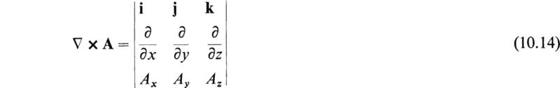
This may be written conveniently in the following determinantal form:
If A = ∇ϕ,
It thus follows that if A is the gradient of a scalar, the curl of A vanishes.
To show the connection between the line integral and the curl of a vector field, let us compute the line integral of a vector field A around an infinitesimal rectangle of side Δx and Δy lying in the xy plane, as shown in Fig. 10.3. That is, we shall compute A·dI around this rectangle. We may write down the various contributions to this integral as follows:
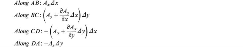
where we have made use of the fact that Δx and Δy are infinitesimals. Adding the various contributions, we obtain
In view of (10.13), this may be written in the form
where ∇× Az is the z component of the curl of A and dsxy is the area of the rectangle ABCD.
Consider now a closed curve in the xy plane, as shown in Fig. 10.4. Divide the space inside C by a network of lines joining a network of infinitesimal rectangles.
Fig. 10.3
Fig. 10.4
If we take the sum of the line integrals around the various meshes, we obtain
Now it is easily seen that the contributions to the line integrals of adjoining meshes neutralize each other because they are traversed in opposite directions; the only contributions which are not neutralized are those on the periphery of the surface. Hence
where the line integral on the right is taken along the boundary curve C in the positive sense.
Now the sum on the right of (10.18) reduces to the following integral:
Hence, substituting this into (10.18), we obtain
That is, the line integral of a vector field A about the contour C of a plane surface S is equal to the surface integral of the normal component of the curl of A to the surface throughout the surface s.
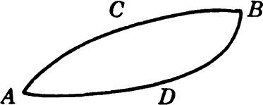
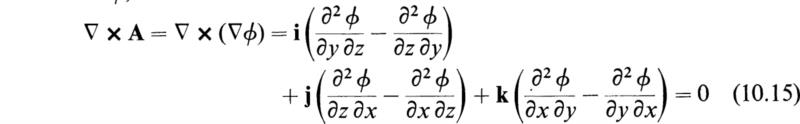
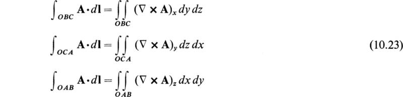
Consider now the triangular surface of Fig. 10.5. It is easy to see that
Fig. 10.5
since the contribution along the lines OA, OB, and OC cancel each other. However, as a consequence of (10.21), we have
If we add these equations and make use of (10.22), we obtain
Now we may write
for the projections of the representative surface vector s of the plane ABC to the yz, xz, and xy planes. Using this notation, (10.24) becomes
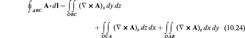
Consider now the open surface of Fig. 10.6. We can regard the surface s of this open surface as being made up of an infinite number of elementary triangular surfaces. If we label r the typical triangle, we have from (10.26)
Now the sum of the line integrals of the elementary triangles reduces to a line integration about the periphery C of the closed surface S since the
Fig. 10.6
line integrations along adjacent triangles are described in opposite senses and hence cancel. We therefore have
In the limit the summation on the right of (10.27) reduces to an integral, and we have
As a consequence of (10.19), we then have
This relation is known as Stokes’s theorem. It states that the surface integral of the curl of a vector field A taken over any surface S is equal to the line integral of A around the periphery of the surface.
If the surface to which Stokes’s theorem is applied is a closed surface, the length of the periphery is zero and then
By the use of Stokes’s theorem we see that, if ∇ × A = 0 everywhere, A is the gradient of a scalar function, because if ∇ × A = 0, then the line integral of A around any closed curve vanishes. This is just the condition that A should be the gradient of a scalar function.
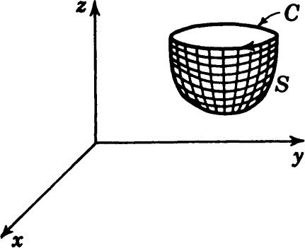
It frequently happens in various applications of vector analysis that we must operate successively with the operator ∇. For example, since the curl of a vector field A, ∇ × A, is a vector field B, it is possible to take the curl of B, that is,
If we expand this equation in terms of the cartesian coordinates of A.we obtain
In the same manner the following vector identities may be established by expanding V and the other vectors concerned in terms of their components:
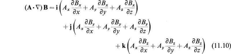
In the above set of equations the symbol (A ∇)B stands for the vector
The above formulas are very useful in applications of vector analysis to various branches of engineering and physics.
Many calculations in applied mathematics can be simplified by choosing instead of a cartesian coordinate system another kind of system that takes advantage of the relations of symmetry involved in the particular problem under consideration.
Let these new coordinates be denoted by u1, u2, u3. These are defined by specifying the cartesian coordinates x, y, z as functions of u1, u2, u3, as follows:
We shall confine ourselves to the case when the three families of surfaces u1 = const, u2 = const, u3 = const are orthogonal to one another. In this case the line element ds is given by
where h1, h2, h3 may be functions of u1, u2, u3. We shall also adopt the convention that the new coordinate system shall be right-handed like the old.
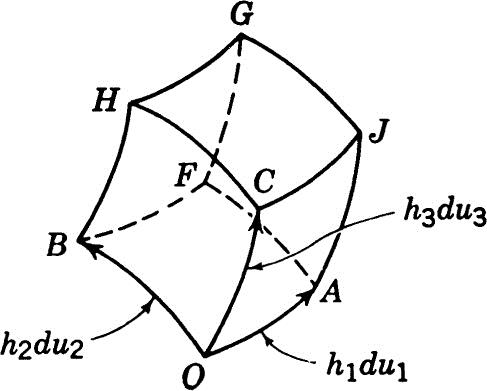
Consider now the infinitesimal parallelepiped whose diagonal is the line element ds and whose faces coincide with the planes u1 or u2 or u3 = const (see Fig. 12.1).
The lengths of its edges are h1 du1, h2 du2, h3du3, and its volume is h1 h2 h3 du1du2du3 Furthermore let ϕ(u1, u2, u3) be a scalar function and A be a vector field with components A1, A2, A3 in the three directions in which the coordinates u1 u2, u3 increase. The u1 component of the gradient of ϕ we can compute at once since by definition
We also have similar relations for the directions 2 and 3.
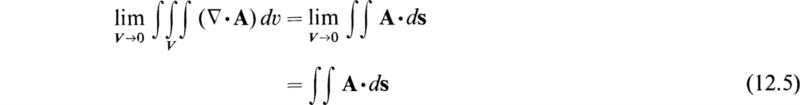
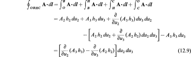
In order to calculate the divergence of a vector field A, we use Gauss’s theorem:
The contribution to the integral ![]() through the area OBHC, taken in the direction of the outward normal, is —A1h2h3du2d3, while that through the area AFGJ is
through the area OBHC, taken in the direction of the outward normal, is —A1h2h3du2d3, while that through the area AFGJ is
![]()
From these and the corresponding expressions for the other two pairs of surfaces, we have by (12.4)
Fig. 12.1
We thus obtain
If A = ∇ϕ,
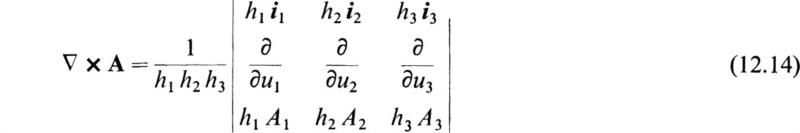
The components of the curl of A may be found by Stokes’s theorem,
For example, the component 1 of the curl of A is obtained by applying Stokes’s theorem to the surface OBHC. We calculate
By Stokes’s theorem this equals the 1 component of the curl of A, (∇ × A)1, multiplied by the area of the face OBHC. That is,
Hence
By a cyclic change of the indices we obtain
If we introduce unit vectors i1, i2, i3 along the directions 1, 2, and 3, we may write symbolically
In the case of cartesian coordinates we have u1 = x, u2= y, u3 = z, h1= h2= h3 = 1, and i1 = i, i2 = j, j3 = k. In this case (12.14) reduces to (10.14). We shall now apply these general formulas to two special cases that are particularly important in applications.
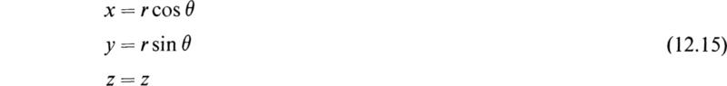
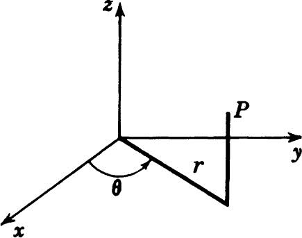
The position of a point in space may be determined by the cylindrical coordinate system of Fig. 12.2. In this case we have
We have, therefore, in this case,
By (12.3) we obtain
By (12.6) we have
Fig. 12.2
The Laplacian operator as given by (12.7) gives
We obtain the components of the curl of A by (12.11), (12.12), and (12.13):
Another very important coordinate system is that of spherical polar coordinates, as shown in Fig. 12.3. In this case we have
We have therefore
Fig. 12.3
Consider a region of space containing a fluid of density ρ(x,y,z,t). Let V be the volume inside an arbitrary closed surface s located in this region. Let Q(t) be the mass of fluid inside the volume Fat any instant. Then
If υ denotes the velocity of a typical particle of the fluid, the rate at which the mass of fluid inside V is increasing is
Now, if we differentiate (13.1) with respect to time and equate the result to (13.2), we have
But, by Gauss’s theorem, we have
Substituting this into (13.3) and transposing, we obtain
Now since the integrand is continuous and the volume V is arbitrary, we conclude that
This is the basic equation of hydrodynamics and is known as the equation of continuity.
If the fluid is incompressible, then ρ is a constant and we have
If the flow is irrotational, then we have
and we know from Sec. 10 that there exists a scalar function ϕ such that
If the fluid is incompressible, then from (13.7) we have
and hence ϕ, called the velocity potential, satisfies the equation
On a fixed boundary of the fluid, the velocity has no normal component, and if ∂/∂n denotes differentiation with respect to the normal direction of the boundary, we must have
as a consequence of (13.9) .
Let us denote any general property of a particle of the fluid, such as its pressure, density, etc., by the function H(x,y,z,t). Then by ∂H/∂t is meant the variation of H at a particular point in space as a function of the time t. If we take the total differential of H(x,y,z,t), we obtain
The quantity dH/dt is the variation of H when we fix our attention on the same particle of fluid.
The velocity of the particle is given by
By definition we have
To obtain the equation of motion of a frictionless fluid, we consider the forces acting on an element of fluid whose volume is dx dy dz and whose mass is ρ dx dy dz. As a consequence of the pressure of the fluid, p, there will be a force in the x direction on the element of fluid under consideration, of magnitude
Let us also consider the action of an external force F acting on unit mass of fluid. The external force acting on the element under consideration in the x direction is Fxρ dx dy dz. The acceleration of the element in the x direction is ![]() Hence, by Newton’s second law of motion, we have
Hence, by Newton’s second law of motion, we have
By this reasoning, and considering the y and z directions, we obtain Euler’s equations of motion:
These three scalar equations may be combined into the single vector equation
As a consequence of Eq. (13.18), we have
Now by the vector identity (11.6), we have
Hence, by the use of the two equations above, we may write Euler’s equation of motion in the following form:
If the external force is conservative, it has a potential V and we have
If the motion of the fluid is irrotational, ∇ × v = 0 and v = ∇ϕ. In this case Eq. (13.25) becomes
or
where
Now if dr denotes an arbitrary path in the fluid at any instant, we have
Let us form the scalar product of ∇w and dr We then obtain
as a consequence of Eq. (13.28). Hence
where β(t) is an arbitrary function of time, since we have integrated along an arbitrary path in the fluid at any instant. That is, we have
Equation (13.32) is known as Bernoulli’s equation.
In the special case where p is constant and the motion is steady so that ∂ϕ/ϕt = 0, this equation takes the form
where β is now a constant. This equation states that, per unit mass of fluid, the sum of the kinetic energy, the potential energy V, and the pressure energy p/ρ has a constant value β for all points of the fluid.
Usually in aerodynamics the variations in V are so small that they can be neglected so that we can write
where p0 is the pressure when the fluid is at rest. It can be seen from this that in this case the pressure diminishes as the velocity increases in the form
Airplanes are equipped with instruments for measuring p and p0 so that the velocity of the machine relative to the air can be determined by the equation
Consider a region inside a solid body such as a large block of metal. Let a closed surface s be situated inside this region. Let the volume inside the surface s be denoted by V.
In suitable units the amount of heat H inside the volume V of this body is given by
where u = u(x,y,z,t) = temperature of body
c = specific heat of body
ρ = density of body
It is an empirical fact that the rate of flow of heat into the volume V may be expressed in the following form:
where k is a constant known as the thermal conductivity and ∂u/∂n is the derivative of the temperature with respect to the outward drawn normal to the surface s.
If we differentiate (14.1) with respect to t and equate the result to (14.2), we obtain
If dn is a vector drawn in the direction of the outward drawn normal to the surface s, we have
where du is the total derivative of the temperature and represents the change in temperature as one moves through the distance dn. If we divide both sides of (14.4) by the differential dn, we obtain
where n represents a unit vector in the normal direction. We then have
If we let
we have, in view of (14.3) and (14.6),
where we have used Gauss’s theorem to transform the last integral. Transposing, we may write
Since the integral is continuous and the volume V is arbitrary, the integrand must vanish and we obtain
or
If k is a constant, we have
where
Equation (14.13) was derived by Fourier in 1822 and is sometimes called the heat-flow, or diffusion, equation.
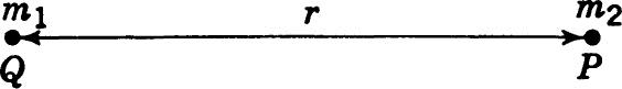
Consider two particles at Q and P of masses m1 and m2, respectively. Then, according to the Newtonian law of gravitation, there is a force of attraction between them given in magnitude by the equation
where k is a constant depending upon the units and r is the distance between the particles as shown in Fig. 15.1.
If we choose the unit of mass as that of a particle which, placed at a unit distance from one of equal mass, attracts it with unit force, Eq. (15.1) becomes
If we denote the vector QP by r, we may express the force per unit mass at P due to the attracting particle at Q by
F is called the intensity of force or the gravitational field of force at the point P, and we note that it may be expressed as the gradient of the scalar m/r. It follows therefore that F satisfies the equation
and is therefore a conservative field of force.
Let us suppose that the particle m is stationary at Q and that another of unit mass moves under the attraction of the former from infinity up to P
Fig. 15.1
along any path. The work done by the force of attraction during an infinitesimal displacement dr of the unit mass is F·dr. The total work done by the force while the unit particle moves from infinity up to P is
This is independent of the path by which the particle comes to P and is called the potential at P due to the particle of mass at Q. Let us denote it by V. We then have
while the intensity of force at P due to it is
That is, the intensity at any point is equal to the gradient of the potential.
If we now suppose that there are n particles of masses m1, m2, . . ,mn, relative to which P has position vectors r1, . . . , rn, respectively, then the force of attraction per unit mass at P due to the system is the vector sum of the intensities due to each, that is,
Now, by the same argument as before, the work done by the attracting forces on a particle of unit mass while it moves from infinity up to P is
Therefore the potential at P due to a system of particles is the sum of the potentials due to each. The potential V is a scalar function of position and, except at the points Qs where the masses are situated, it satisfies
which is Laplace’s equation. Since F = ∇V, this means that at points excluding matter we must have
Let us now suppose that the attracting matter forms a continuous body filling the space bounded by the closed surface s. We divide the body into an infinite number of elements of mass ρdV, where ρ is the density of the body and dV is the element of volume of the body, as shown in Fig. 15.2.
If P is outside the body, the sum in Eq. (15.9) passes into the integral
where r is the distance from the element of volume dV to the point P. gives the point P. This potential at P due to the entire body.
If the point P is inside the body, the integrand (15.12) becomes infinite. In this case we define the potential in the following manner: Surround the point P by a closed spherical surface s0, and consider the potential due to the matter in the space between s0 and s. The integrand is finite everywhere, since P is outside the region. Now let the surface s0 decrease indefinitely, converging to the point P as a limit.
We then consider
Since the volume of s0 is of the same order as r3, where r is the radius of the sphere s0, while the integrand becomes infinite like 1/r if ρ is finite, the value of the above integral tends to a definite limit, which is called the potential at P due to the whole body.
We have seen that the potential function satisfies ∇2V = 0, or Laplace’s equation, in the region outside matter. Let us now consider the equation satisfied by the potential in a region inside matter. Consider a point P inside a body of density ρ. Surround the point P by a sphere s0 of radius a, as shown in Fig. 15.3.
The gravitational field at the point P is the vector sum of the gravitational field F0 produced by the matter outside s0 and Fi produced by the matter inside s0. That is, we write
Fig. 15.2
Fig. 15.3
Now let us calculate ∇·FP, that is,
But since F0 is produced by matter outside s0, we have from (15.11)
Hence we have
Consider the sphere of radius a; its mass is therefore equal to
Now as a tends to zero, the intensity at the surface of this sphere is equal to
in magnitude and in the direction of the inwardly drawn normal to the surface. By Gauss’s theorem we then have
Hence
But
![]()
Hence by (15.21) the equation satisfied by the potential in a region containing matter is
This relation is known as Poisson’s equation. In view of (15.13) we see that we may take
as a solution of Poisson’s equation.†
As a consequence of Poisson’s equation we may prove that the surface integral of the gravitational force F over a closed surface s drawn in the field is equal to –4π times the total mass enclosed by the surface.
To establish this, apply Gauss’s theorem to Eq. (15.22); we then have
But ∫ ∫ ∫ ρ dv is the total mass enclosed by the surface s. This theorem has many applications in potential theory and in the theory of electrostatics.
The study of electrodynamics affords one of the most important applications of vector analysis. According to the modern point of view, by an electromagnetic field is understood the domain of the five vectors E, B, D, H, and J. These vectors satisfy the differential equations
and in a homogeneous isotropic medium we have the additional relations
The above set of differential equations are the fundamental equations of Maxwell written in a rationalized mks system of units. In this system of units we have
E = electric intensity, volts per m
B = magnetic induction, webers per m
D = electric displacement, coulombs per m2
H = magnetic intensity, amp per m
J = current density, amp per m2
σ = electric conductivity, 1/ohm-m
K= KrK0 = electric inductive capacity of medium
μ = μrμ0 = magnetic inductive capacity of medium
Kr = dielectric constant
μr = permeability
K0 = 8.854 × 10¹² farad per m
μ0 = 4π× 10–7 = 1.257 × 10⁻⁶ henry per m
ρ = charge density, coulombs per m3
c = ![]() = 2.998 × 10⁸ m per sec
= 2.998 × 10⁸ m per sec
The solution of electrodynamic problems depends on the solution of these equations in special cases. For example, we may discuss briefly the following special cases.
In the case that the field vectors are independent of the time and in a region where J = 0, we see that all the terms involving partial derivatives with respect to time vanish and the electric vectors and magnetic vectors become independent of each other. We then have
and
Since the curls of E and H vanish, we see that both these fields may be derived from potential functions. It is conventional to write
where VE and VM are the electric and magnetic scalar potentials, respectively.
In view of (16.9) and (16.12) we see that these potentials satisfy the equations
and
That is, the electric potential satisfies Poisson’s equation, and the magnetic potential satisfies Laplace’s equation. If the charge density ρ vanishes, then both VE and VM satisfy Laplace’s equation and the solution of electrostatic and magnetostatic problems reduces to the solution of this equation subject to the proper boundary conditions.
Let us eliminate the magnetic-intensity vector H from the Maxwell field equations. To do this, let us take the curl of both sides of Eq. (16.1); we then have
in view of the fact that B = μH and that the operators ∇ × and ∂/∂t commute.
Equation (16.2) may be written in the form
Substituting this into (17.1) and making use of the identity
we obtain
Now, in view of (16.4), we have
and it may be shown that in free space or in a conducting medium ρ is independent of the field distribution and may be taken to be equal to zero. Accordingly, Eq. (17.4) becomes
As a consequence of (16.7) we also have
Eliminating E from the Maxwell equations, we also obtain
It is thus seen that the three vectors H, E, and J satisfy equations of the same form.
In free space we have the conductivity σ = 0 and μr = Kr = 1; we then obtain
and
If we let
We may write (17.9) in the form
This equation is the general wave equation in vector form and is discussed in Chap. 12. It is there shown that this equation governs the propagation of various entities, such as electric waves, displacements of tightly stretched strings, deflections of membranes, etc. It will be shown that such disturbances are propagated with a velocity equal to c.
Equations (17.9) and (17.10) are taken as the starting point in the theory of electromagnetic waves. In this case, c is the velocity of light in free space and is approximately 3 × 10⁸ m per sec.
In metals σ is of the order of 107(l/ohm-m) and ![]() r ≈ 1, and it may be seen that the term involving the second derivative in (17.7) may be neglected for frequencies of the order of 1010 cycles per sec and lower. In such a case this equation reduces to
r ≈ 1, and it may be seen that the term involving the second derivative in (17.7) may be neglected for frequencies of the order of 1010 cycles per sec and lower. In such a case this equation reduces to
We thus see that the current density in metals satisfies an equation of the same form as is satisfied by the equation of heat flow in solids as given in Sec. 14. In the electrical-engineering literature this equation is called the skin-effect equation. The solution of this equation in various special cases is considered in Chap. 11.
In many physical problems vector notation is not sufficiently general to express the relations between the quantities involved. For example, in electrostatics, if a dielectric medium is isotropic, the relation between the electric-displacement vector D and the electric-intensity vector E is given by the vector equation
where the scalar K is the electric inductive capacity of the medium (see Sec. 16). If, however, the dielectric medium is not isotropic, the electric-displacement vector D does not have the same direction as the vector E, so that the scalar K must be replaced by a more general quantity to effect the required change in direction and magnitude. Such a quantity is called a tensor.
A similar situation arises in the formulation of elastic problems. If F is the stress vector in an isotropic medium and X is the strain vector, then the relation
where k is a scalar, exists. If the medium is not isotropic, F and X are no longer in the same direction and Eq. (19.2) takes on a more general form in which k is a tensor.
After this qualitative introduction, the simpler analytical properties of tensors will be discussed in the following sections.
The fundamental definitions involved in the calculus of tensors or tensor analysis are intimately connected with the subject of coordinate transformations. In this section some of the fundamental properties of these transformations will be discussed.
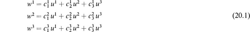
Consider a set of variables (u1,u2,u3) related to another set of variables (w1,w2,w3). (The superscripts denote different variables and not the powers of the variables involved.) Let the relation between the two sets of variables be of the form
where the coefficients ![]() are constants. In this case the variables (u1,u2,u3) are related to the variables (w1,w2,w3) by a linear transformation. This transformation may be expressed by the equation
are constants. In this case the variables (u1,u2,u3) are related to the variables (w1,w2,w3) by a linear transformation. This transformation may be expressed by the equation
For convenience, in tensor analysis, the following summation convention has been adopted:
The repetition of an index in a term once as a subscript and once as a superscript will denote a summation with respect to that index over its range. In (20.2) the range of n is from 1 to 3, so that, by the above summation convention, (20.2) may be written in the form
The determinant ![]() is the determinant of the linear transformation (20.1). If C≠0, the transformation will have an inverse. Let
is the determinant of the linear transformation (20.1). If C≠0, the transformation will have an inverse. Let ![]() be the cofactor of
be the cofactor of ![]() in the determinant C, divided by C. Then, by Chap. 2, Eq. (4.8), we have
in the determinant C, divided by C. Then, by Chap. 2, Eq. (4.8), we have
The symbol ![]() is called a Kronecker delta and has the values indicated in (20.4). In order to solve the system of Eqs. (20.1), multiply both sides by b\ and obtain
is called a Kronecker delta and has the values indicated in (20.4). In order to solve the system of Eqs. (20.1), multiply both sides by b\ and obtain
Therefore the solution of the system (20.3) is
and therefore the transformation (20.1) is reversible.
Consider the two linear transformations
and
where all the indices range from 1 to n. If (20.7) is substituted into (20.8), the result is
where
is the transformation matrix of the linear transformation (20.9). These linear transformations may also be expressed by means of the matrix notation of Chap. 3 in the following form:
Therefore
where the matrices (x), (y), (z) are column matrices of order n and the matrices [a], [b], and [c] are square matrices of order n.
Consider a three-dimensional Euclidean space. The position of a point P in this space can be specified by its coordinates referred to an orthogonal cartesian system of axes. Let (y1,y2,y3) denote such a system of coordinates. Let
be a transformation of coordinates from the rectangular cartesian coordinates (y1,y2,y3) to some general coordinates (x1,x2,x3), not necessarily rectangular cartesian coordinates. For example, (x1,x2, x3) may be spherical coordinates. The inverse of the transformation of coordinates (20.13) is the transformation that takes one from the coordinates (x1,x2,x3) to the rectangular cartesian coordinates (y1,y2,y3). Let
be the inverse of the coordinate transformation (20.13). When this transformation exists, it is seen that to each set of values yr there is a unique set of values of xr, and vice versa. Hence the variables xr determine a point in space uniquely and they are called curvilinear coordinates.
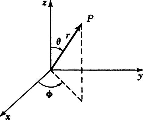
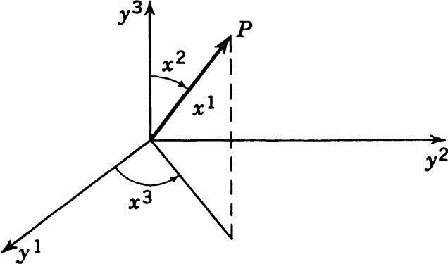
The spherical polar coordinates of Sec. 12 may be taken as a special example of the general transformations (20.13) and (20.14). In this notation, consider the spherical polar coordinates of Fig. 20.1. In this figure y1, y2, y3 are the cartesian coordinates of a point P, and x1, x2, x3 are the spherical polar coordinates of P. x1 is the radius vector from the origin to the point P, and
Fig. 20.1
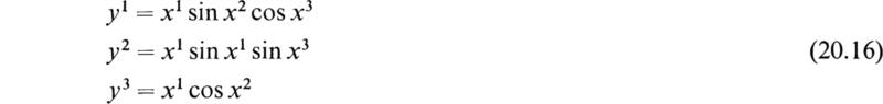
x2 and x3 are the angles shown in Fig. 20.1. In this special case the transformation (20.13) takes the form
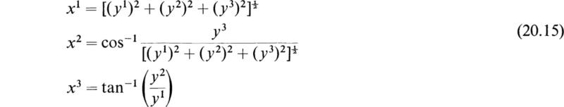
The inverse transformation (20.14) in this case takes the following form:
The fundamental types of tensors will now be defined with respect to functional transformations from one set of curvilinear coordinates to another. The discussion of tensors with respect to general functional transformations follows the same fundamental principles and may be carried out by considering a space of n dimensions.
Let a Euclidean space be specified by the curvilinear coordinates (x1,x2,x3). Let new curvilinear coordinates ![]() be introduced by the transformation
be introduced by the transformation
Let a quantity have the value N in the old variables xr and the value ![]() in the new variables
in the new variables ![]() . Then, if the quantity has the same value in both sets of variables so that
. Then, if the quantity has the same value in both sets of variables so that
the quantity N is called a scalar, or an invariant, or a tensor of order zero.
b CONTRAVARIANT VECTORS
Let three quantities have the values (A1,A2,A3) when expressed in terms of the coordinates (x1,x2,x3), and let these quantities have the values ![]() when expressed in the coordinates
when expressed in the coordinates ![]() If
If
then the quantities (A1,A2,A3) are said to be the components of a contra-variant vector or a contravariant tensor of the first rank with respect to the transformation (21.1).
Taking differentials on both sides of (21.1),
Since the components of an ordinary vector in three-dimensional space transform as the differentials of the coordinates, it is seen that the components of an ordinary vector are actually the components of a contravariant tensor of rank 1.
If three quantities have the values (A1,A2,A3) in the system of coordinates (x1,x2,x3) and the values ![]() in the system of coordinates
in the system of coordinates ![]() and if
and if
then (A1A2,A3) are the components of a covariant vector or a covariant tensor of rank 1.
In the above three classes of quantities, scalars or invariants, contravariant and covariant vectors, there exist components in any two coordinate systems, and the components in any two coordinate systems are related by the defining laws of transformation. There are other quantities whose components in any two coordinate systems are related by characteristic laws of transformation. These laws of transformation are involved in the definitions of tensors of higher ranks. There are three varieties of second-rank tensors:
The A’s with the bars denote components in the coordinates ![]() and those without the bars denote components in the coordinates (x1,x2,x3).
and those without the bars denote components in the coordinates (x1,x2,x3).
Tensors of higher rank are defined by similar laws; for example, a mixed tensor of rank 4 is
A very useful mixed tensor of the second rank is the Kronecker delta ![]() This is defined by the equation
This is defined by the equation
To determine whether ![]() is a mixed tensor of the second rank, we investigate whether it satisfies the definition (21.8).
is a mixed tensor of the second rank, we investigate whether it satisfies the definition (21.8).
But
since ![]() and
and ![]() are independent variables. Hence
are independent variables. Hence
We thus see that ![]() has the same components in all coordinate systems. The relation
has the same components in all coordinate systems. The relation
is a very useful one.
It can be easily shown that the sum or difference of two or more tensors of the same rank and type is a tensor of the same rank and type. For example, if
it follows from (22.1) that Cmn is a contravariant tensor of the second rank.
If the contravariant tensor Am is multiplied by the covariant tensor Bn, the product is the following mixed tensor of the second rank:
It is easy to see that ![]() transforms like (21.8). The product (22.2) is called the outer product. It may be obtained with tensors of any rank or type. For example, the tensor
transforms like (21.8). The product (22.2) is called the outer product. It may be obtained with tensors of any rank or type. For example, the tensor ![]() may be multiplied by the tensor Bpq to obtain the following outer product:
may be multiplied by the tensor Bpq to obtain the following outer product:
Consider the mixed tensor ![]() and let the index m be set equal to n so that m = n. The law of transformation (21.8) now gives the result
and let the index m be set equal to n so that m = n. The law of transformation (21.8) now gives the result
and hence ![]() is a scalar. This process of summing over a pair of contra-variant and covariant indices is called contraction. As another example, consider the mixed tensor
is a scalar. This process of summing over a pair of contra-variant and covariant indices is called contraction. As another example, consider the mixed tensor ![]() and let m = q. Let Bnp =
and let m = q. Let Bnp = ![]() The law of transformation now gives
The law of transformation now gives
Therefore ![]() is a covariant tensor of rank 2. The process of contraction always reduces the rank of a mixed tensor by 2.
is a covariant tensor of rank 2. The process of contraction always reduces the rank of a mixed tensor by 2.
If two tensors are multiplied together and then contracted, the result is called the inner product. For example, the inner product is
The inner product of Amn and Brpq is
The product Am Bm is equivalent to the scalar product of two vectors in rectangular coordinates. In tensor analysis the length L of the tensor Am or Am is defined by the equation
The scalar product of the two vectors Am and Bm is
where θ is the angle between the vectors Am and Bm. Hence
If Am and Bm are orthogonal, then
It can be shown by applying the law of transformation of tensors that, if the following relation exists,
where Cr is known to be a tensor and Bst is a known arbitrary tensor, then A(r,s,t) is a tensor of the rank
This law is of importance in recognizing tensors.
Let the cartesian coordinates of the point P be yr. The element of length dS of such a coordinate system is given by
Since the cartesian coordinates are related to the general coordinates xi by the functional relations
we have
It therefore can be seen that
where
This equation shows that gmn is symmetric, and since dS is an invariant for arbitrary values of the contravariant vector dxm, it follows from the quotient law that gmn is a double covariant tensor. The tensor gmn is called the fundamental, or metric, tensor. Let g denote the determinant |gmn| and Gmn denote the cofactor of gmn in g. We now define the quantity gmn by the equation
Now, from the theory of determinants [see Chap. 2] we have
Hence by the quotient law it can be seen that gmn is a double contravariant tensor of rank 2.
Two vectors related by the following equations,
and
are called associated vectors. In the literature of tensor analysis it is sometimes said that Am and Am are the same vector, Am being the contravariant components and Am the covariant ones. Besides the fundamental, or metric, tensor gmn and the second fundamental tensor gmn there is the third associated tensor, ![]() defined by the equation
defined by the equation
This relation follows from (23.9).
Associated tensors of any rank may be obtained in the same manner as (23.10) and (23.11). For example,
If we are given a contravariant vector Ar, we can form an invariant A by means of the equation
A is called the magnitude of the vector A. In the same manner the magnitude B of the covariant vector Bm is defined by the equation
A unit vector is one whose magnitude is unity. If (23.6) is divided by ![]() we have
we have
From this it can be concluded that dxm/dS is a unit vector. By the use of (22.9) and (23.11) it can be shown that the angle θ between the vectors Am and Bm may be expressed in the form
Let ϕ be an invariant function of a parameter t; then, in the new variables ![]() we have
we have ![]() and it can be shown that
and it can be shown that
so that dϕ/dt is also an invariant. If ϕ is an invariant function of xr, we have
This shows that ∂ϕ/∂xr is a covariant vector since it transforms like one.
In Sec. 24 it has been shown that the derivative of a scalar point function is a covariant vector. However, the derivative of a covariant vector is not a tensor, for if
the derivative of Ām with respect to ![]() is
is
The presence of the second derivative shows that ∂Am/∂xn does not transform like a tensor.
In order to define “derivatives” of tensors that preserve the proper tensor character, it is necessary to introduce the following notation:†
and
The quantity [mn,p] is called the Christoffel symbol of the first kind, and ![]() is called the Christoffel symbol of the second kind.
is called the Christoffel symbol of the second kind.
It can be shown that the quantity
is a contravariant vector. This vector is defined to be the intrinsic derivative of the vector Ar with respect to the parameter t.
The quantity
can be shown to be a covariant vector and is defined to be the intrinsic derivative of Ar with respect to the parameter t.
The covariant derivative of the contravariant vector Ar with respect to the coordinate xs is defined by the equation
This quantity can be shown to be a mixed tensor contravariant in r and covariant in s. The covariant derivative of the covariant vector Ar with respect to the coordinate xs is defined by the equation
This quantity can be shown to be a tensor covariant in both r and s.
The intrinsic derivative of the tensor ![]() with respect to the parameter t is defined by the equation
with respect to the parameter t is defined by the equation
It can be shown that this quantity is a tensor of the type ![]()
The covariant derivative of the tensor ![]() with respect to the variable xn is defined by the equation
with respect to the variable xn is defined by the equation
This is a tensor with one covariant index more than ![]() The definitions of the intrinsic and covariant derivatives are quite general. Terms of the forms (25.5) and (25.7) appear in the derivatives of a mixed tensor for each contravariant index, and terms of the forms (25.6) and (25.8) appear in the derivatives of mixed tensors for each covariant index.
The definitions of the intrinsic and covariant derivatives are quite general. Terms of the forms (25.5) and (25.7) appear in the derivatives of a mixed tensor for each contravariant index, and terms of the forms (25.6) and (25.8) appear in the derivatives of mixed tensors for each covariant index.
If the coordinate system is a rectangular cartesian one, the gmn quantities are all constants and the Christoffel systems are identically zero. In such case the intrinsic derivatives are identical to the ordinary derivatives, and the covariant derivatives are ordinary partial derivatives.
The fundamental, or metric, tensor grs has components that are constants in cartesian systems, and therefore
in such a system. Since grs is a tensor, it follows that, in every coordinate system, the following equation must be satisfied:
Therefore the covariant derivative of the metric tensor grs is zero. It can also be shown that the covariant derivative of the associated tensor grs is zero.
In the brief introduction to the basic ideas and definitions of tensor analysis given in this appendix, space does not permit the discussion of numerous applications to applied mathematics. These applications will be found in the treatises on tensor analysis listed in the references at the end of this chapter. For purposes of illustration, however, a brief discussion of the application of tensor analysis to the dynamics of a particle will be given in this section.
Consider a particle of mass M that is moving in space. Let the position of this particle be given by a system of curvilinear coordinates xr. As the time t varies, the particle will describe a certain curve in space, called the trajectory of the particle. The equations of this curve may be written in the form
If we transform to another curvilinear coordinate system ![]() in accordance with the transformation
in accordance with the transformation
then the trajectory of the particle may be obtained in terms of t by substituting (27.1) into (27.2).
Consider the quantity
In the new coordinates ![]() the corresponding quantities are
the corresponding quantities are
This equation expresses the fact that the υr are the components of a contra-variant vector. In dynamics this vector is called the velocity of the particle. The velocity vector υr is a function of the time t. If the intrinsic derivative with respect to t is taken, the following result is obtained:
where ![]() are the Chistoffel symbols of the coordinate system xr..
are the Chistoffel symbols of the coordinate system xr..
If the coordinates are rectangular cartesian, the Christoffel symbols are identical to zero and the vector ar becomes
These are the components of acceleration along the three coordinate axes; (27.5) is called the acceleration vector of the particle. If the mass of the particle M remains constant, it is obviously a quantity independent of the coordinate system and the time and is, therefore, an invariant.
Newton’s second law of motion may be expressed in the form
where the contravariant vector Fr is called the force vector. This vector completely specifies the magnitude and direction of the force acting upon the particle. In cartesian coordinates (27.7) takes the well-known form
and F1, F2, F3 are the components of the force along the three axes of coordinates. In curvilinear coordinates this equation takes the form
If the axes ![]() are rectangular cartesian, a force whose components in these coordinates are
are rectangular cartesian, a force whose components in these coordinates are ![]() and whose point of application is moved through a small displacement
and whose point of application is moved through a small displacement ![]() does an amount of work given by
does an amount of work given by
In orthogonal cartesian coordinates the associated vector ![]() has exactly the same components as
has exactly the same components as ![]() and the expression for δ W becomes
and the expression for δ W becomes
From the relation connecting ![]() and
and ![]() it can be seen that δW can also be written in the form
it can be seen that δW can also be written in the form
Since δW is an invariant, it can be concluded from the above equation that the Fr are the components of a covariant vector. Since the components of Fr in an orthogonal cartesian coordinate system are those of the force vector, it follows that Fr is the covariant force vector in the coordinates xr.
The covariant and contravariant components of this vector are related to each other by the following formulas:
If the expression Frdxr is a perfect differential, then the force is said to be conservative and a function V may be defined by the equation
The function V is called the force potential. From (27.14) it follows that
The kinetic energy T of a particle is defined as ![]() , where υ is the magnitude of the velocity. Therefore
, where υ is the magnitude of the velocity. Therefore
where gmn is the metric tensor of the curvilinear coordinates xm.
If T is differentiated partially with respect to ![]() r, the result is
r, the result is
Therefore
Also, if T is differentiated partially with respect to xr, the result is
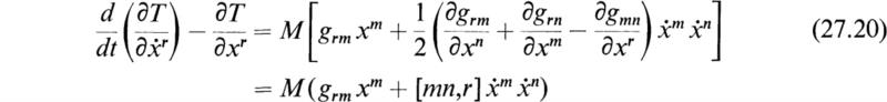
From (27.18) and (27.19) it can be deduced that
where [mn,r] is the first Christoffel symbol. Therefore
As a consequence of (27.5) it can be seen that the right-hand member of (27.21) is equal to Mgrsas = Mar. Therefore (27.21) may be written in the form
These are Lagrange’s equations. If the force system is conservative, these equations may be written in the form
1. The point of application of a force F = 5, 10, 15 lb is displaced from the point (1,0,3) to the point (3,–1,–6). Find the work done by the force.
2. Find the scalar product of two diagonals of a unit cube. What is the angle between them?
3. A force F acts at a distance r from the origin. Show that the torque L about any axis through the origin is L = (r × F) a when a is a unit vector in the direction of the axis.
4. Show that the lines joining the midpoints of the opposite sides of a quadrilateral bisect each other.
5. Show that the bisectors of the angles of a triangle meet at a point.
6. What is the cosine of the angle between the vectors A = 4i + 6j + 2k and B = i – 2j + 3k ?
7. Let r be the radius vector from the origin to any point and a constant vector. Find the gradient of the scalar product of a and r.
8. A plane central field A is defined by A = rF(r). Determine F(r) so that the field may be irrotational and solenoidal.
9. A central field A in space is defined by A = rF(r). Determine F(r) so that the field may be irrotational and solenoidal.
10. If r is a unit vector of variable direction, the position vector of a moving point may be written r = rr. Find by vector methods the components of the acceleration F parallel and perpendicular to the radius vector of a particle moving in the xy plane.
11. Prove that the vector ∇ϕ is perpendicular to the surface ϕ(x,y,z) = const.
12. Find ∇u if u = In(x2 + y2 + z2).
13. Show that if r is the position vector of any point of a closed surface s, then
![]()
where V is the volume bounded by s.
14. Show that a vector field A is uniquely determined within a region V bounded by a surface S when its divergence and curl are given throughout V and the normal component of the curl is given on S.
15. With every point of a curve in space there is associated a unit vector t the direction of which is that of the velocity of a point describing the curve. This vector therefore has the direction of the tangent. Prove that t·dt/ds = 0, where s is the length of the arc of the curve measured from a fixed point on it. What is the geometrical meaning of dt/ds ?
16. The expression for (ds)2 is (ds)2 = (u2 + v2)[(du)2 + (dv)2] + u2v2(dϕ)2 in parabolic coordinates. What is the form assumed by Laplace’s equation in these coordinates?
17. Write the heat-flow equation in cylindrical and spherical coordinates.
18. What form does the general wave equation take in cylindrical coordinates?
19. Write Maxwell’s equations in cylindrical coordinates.
20. Show that the potential due to a solid sphere of mass M and uniform density at an external point at a distance r from the center is M/r and, hence, that the gravitational intensity is M/r2 toward the center.
21. Show that the gravitational field inside a homogeneous spherical shell is zero.
22. Find the potential inside a solid uniform sphere and the gravitational force inside the sphere.
23. Find the covariant components of the acceleration vector in spherical coordinates.
24. Show that the velocity vector is given by (1/M)grs(∂T/∂![]() s).
s).
25. If ϕ is an invariant function of xr and ![]() r, show that the partial derivative of
r, show that the partial derivative of ![]() with respect to
with respect to ![]() r is a covariant vector.
r is a covariant vector.
26. If a particle is moving with uniform velocity in a straight line prove that δυr/δt = 0.
27. Find the contravariant components of the acceleration vector in cylindrical coordinates.
1901. Gibbs, J. Willard, and Edwin Bidwell Wilson: “Vector Analysis,” Yale University Press, New Haven, Conn.
1911. Coffin, Joseph George: “Vector Analysis,” John Wiley & Sons, Inc., New York.
1928. Weatherburn, C. E.: “Advanced Vector Analysis with Application to Mathematical Physics,” George Bell & Sons, Ltd., London.
1928. Weatherburn, C. E.: “Elementary Vector Analysis with Applications to Geometry and Physics,” George Bell & Sons, Ltd., London.
1931. McConnel, A. J.: “Applications of the Absolute Differential Calculus,” Blackie & Son, Ltd., Glasgow.
1931. Wills, A. P.: “Vector Analysis with an Introduction to Tensor Analysis,” Prentice-Hall, Inc., Englewood Cliffs, N.J.
1932. Gans, Richard: “Vector Analysis with Applications to Physics,” Blackie & Son, Ltd., Glasgow.
1946. Brillouin, L.: “Les Tenseurs en mécanique et en élasticité,” Dover Publications, Inc., New York.
1951. Sokolnikoff, I. S.: “Tensor Analysis,” John Wiley & Sons, Inc., New York.
† This product is commonly called the scalar triple product and is denoted by (ABC).
† See J. L. Synge and B. A. Griffith, “Principles of Mechanics,” 1st ed., Chap. 13, McGraw-Hill Book Company, New York, 1942.
† For a more rigorous derivation of Poisson’s integral, refer to O. D. Kellogg, “Foundations of Potential Theory,” Springer-Verlag OHG, Berlin, 1929.
† See A. J. McConnel, “Applications of the Absolute Differential Calculus,” pp. 143–150, Blackie & Son, Ltd., Glasgow, 1931.