In this chapter solutions of the so-called “wave equation” in simple cases will be considered. One of the most fundamental and common phenomena that occur in nature is the phenomenon of wave motion. When a stone is dropped into a pond, the surface of the water is disturbed and waves of displacement travel radially outward; when a tuning fork or a bell is struck, sound waves are propagated from the source of sound. The electrical oscillations of a radio antenna generate electromagnetic waves that are propagated through space. These various physical phenomena have something in common. Energy is propagated with a finite velocity to distant points, and the wave disturbance travels through the medium that supports it without giving the medium any permanent displacement. We shall find in this chapter that whatever the nature of the wave phenomenon, whether it be the displacement of a tightly stretched string, the deflection of a stretched membrane, the propagation of currents and potentials along an electrical transmission line, or the propagation of electromagnetic waves in free space, these entities are governed by a certain differential equation, the wave equation. This equation has the form
where c is a constant having dimensions of velocity, t is the time, x, y, and z are the coordinates of a cartesian reference frame, and u is the entity under consideration, whether it be a mechanical displacement, or the field components of an electromagnetic wave, or the currents or potentials of an electrical transmission line.
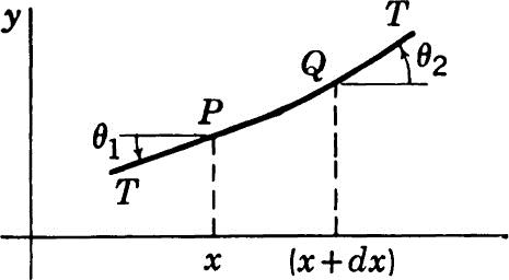
The study of the oscillations of a tightly stretched string is a fundamental problem in the theory of wave motion. Consider a perfectly flexible string that is stretched between two points by a constant tension T so great that gravity may be neglected in comparison with it. Let the string be uniform and have a mass per unit length equal to m. Let us take the undisturbed position of the string to be the x axis and suppose that the motion is confined to the xy plane.
Consider the motion of an element PQ of length ds, as shown in Fig. 2.1. The net force in the y direction, Fy is given by
Now, for small oscillations, we may write
Hence we have
Fig. 2.1
where we have neglected terms of order dx2 and higher. Substituting this into (2.4), we get
By Newton’s law of motion we have
where mdx represents the mass of the section of string under consideration and where we have written dx for ds since the displacement is small. ∂2y/∂t2 is the acceleration of the section of string in the y direction. We thus have
as the equation governing the small oscillations of a flexible string.
If the stretching force is constant throughout the string, we may write
or
This is a special case of the general wave equation (1.1), where in this case we have
It is easy to show that the constant c has dimensions of length/time and hence the same dimensions as a velocity.
We may obtain a general solution of (2.10) by a symbolic method in the following manner: If we write
then Eq. (2.10) may be written symbolically in the form
Let us now treat Eq. (3.2) as an ordinary differential equation with constant coefficients of the form
where
The solution of (3.3) if a were a constant would be of the form
where A1 and A2 are arbitrary constants. Thus Eq. (3.3) is formally satisfied by
where, since the integration has been performed with respect to t, instead of the arbitrary constants A1 and A2 we have the arbitrary functions of x, F1(x) and F2(x). To interpret the solution, we use the symbolic form of Taylor’s expansion, as written in Appendix C.
If we let
we have
If we let
we have
Hence, by (3.6), the general solution of the one-dimensional wave equation (2.10) is given by
Now if F1(x + ct) is plotted as a function of x, it is exactly the same as F1(x) in shape, but every point on it is displaced a distance ct to the left of the corresponding point in F1(x). The function F1(x + ct) thus represents a wave of displacement of arbitrary shape traveling toward the left along the string with a velocity equal to c. In the same manner it may be seen that F2(x – ct) represents a wave of displacement traveling with a velocity c to the right along the string. The general solution is the sum of these two waves.
Consider a string having one end fixed at the origin, and let the other end be a great distance away at x = s. Suppose that a wave of arbitrary shape given by
is approaching the origin. At the origin the displacement must be zero for all time t; hence the reflected wave must have the form
since the sum of this and the original expression is zero at x = 0 for all values of t. This shows that the transverse waves in a stretched string are inverted by reflection from a fixed end.
Consider the expression
By plotting the expression as a function for x for successive values of t it may be shown to represent an infinite train of progressive harmonic waves. It is seen that, as t increases, the whole wave profile moves forward in the positive x direction with a velocity equal to c. The wavelength, that is, the distance between two successive crests at any time, is given by
The time that it takes a complete wave to pass a fixed point is called the period and is given by T. The frequency of the wave is denoted by f and is given by
The wave number, the number of waves that lie in a distance of 2π units, is denoted by k and is given by the equation
The general solution of the wave equation for the vibrating string shows clearly the wave nature of the phenomenon but is not very well suited for certain types of physical investigations.
Consider a string fastened at x = 0 and x = s to fixed supports, and let us suppose that at t = 0 we are given the displacement and velocity of every point of the string. That is, we stipulate that
where y0(x) and υ0(x) are the initial displacement and velocity of the string, respectively.
We then wish to determine the subsequent behavior of the string. To do this, let us assume a solution of the form
where υ(x) is a function of x alone and ω is to be determined. We thus have
On substituting these expressions into the wave equation
it becomes, after some reductions,
This ordinary differential equation has the solution
However, since the string is fastened at x = 0 and at x = s, we have the boundary conditions
The first condition leads to
Since we are looking for a nontrivial solution, A≠0; therefore
This transcendental equation leads to the possible values of ω. Therefore we have
or
where we have labeled ωk the value corresponding to the particular value of k:. For each value of k we may write in view of (5.7) and (5.9) the equation
As a consequence of (5.2) we have for every value of k the solution
This expression satisfies the wave equation (5.5) and the boundary conditions (5.8). Since the real and imaginary parts of (5.15) satisfy the wave equation and the equation is linear, we may write
where Ck and Dk are arbitrary constants.
By summing over all the values of k we can construct a general solution of the form
The arbitrary constants Ck and Dk must now be determined from the initial conditions (5.1). We thus have at t = 0
This requires the expansion of an arbitrary function, y0(x), the initial displacement into a series of sines. To obtain the typical coefficient Cr, we multiply both sides of (5.18) by the expression
and integrate with respect to x from x = 0 to x = s. We then have
If we now make use of the result
then (5.20) reduces to
or
This determines the arbitrary constants Ck in the general solution (5.17). To determine the arbitrary constants Dk, we make use of the second initial condition (5.1). We then have, on computing ∂y/∂t from (5.17) and putting t=0,
Proceeding in the same manner as before, we obtain
for the Dk coefficients.
From (5.23) and (5.25) we see that if the string has no initial velocity the Dk constants are all zero, while if the string has no initial displacement all the Ck coefficients are zero.
Each term of (5.17) represents a stationary wave; the wavelengths are given by 2s/n, where n is any integer. The frequency, or number of periods per second, of the fundamental note is given by
and the frequency of the harmonics, as the other terms are called, is given by
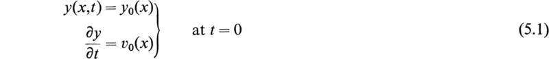
As an example of the application of Eqs. (5.23) and (5.25), let us consider the case of a string that is plucked at its midpoint as shown in Fig. 5.1. In this case, we have the initial condition
Hence by (5.25) we have
The initial displacement y0(x) is given by
Substituting the analytical expression for the initial displacement into Eq. (5.22), we obtain
On carrying out the integrations, we obtain
Substituting these results into (5.17), we obtain the following expression for the displacement of the string on being released from the initial position given by Fig. 5.1:
It is thus seen that no even harmonics are excited and that the second harmonic has one-ninth the amplitude of the fundamental. It is shown in treatises on sound that the energy emitted by an oscillating string as sound is
Fig. 5.1
proportional to the square of the amplitude of the oscillation. It is thus evident that in this case the fundamental tone will appear much louder than the harmonic tone.
In the last section a general solution of the wave equation of the vibrating string was constructed by assuming a solution of the form
This assumption, on substitution into the one-dimensional wave equation, led to the ordinary differential equation
where k is given by
The general solution of (6.2) may be written in the form
Every solution of this form is perfectly acceptable as far as the differential equation is concerned, but it does not describe the behavior of the string. This solution permits the ends of the string to vibrate, whereas the physical condition of the problem requires these to be fixed. It is thus necessary to impose the following boundary conditions upon the solution (6.4):
The boundary conditions may, of course, be satisfied by placing A = 0 and B = 0, but this would lead to the trivial and unwanted solution y = 0 everywhere. Hence there is left only the arbitrary constant B for adjustment. It must be taken to be zero in order to satisfy the first condition of (6.5). However, the function
will not satisfy the second condition of (6.5). The problem can be solved only if we are willing to prescribe only certain values to the undetermined constant k. If sinks must be zero, then k must be 0, or π/s,2π/s, . . . , nπ/s. The value k = 0 is rejected because it leads to the trivial solution y = 0.
The permissible values of k,
are called eigenvalues in the modern literature of mathematical physics. To each eigenvalue there corresponds an eigenfunction
The eigenfunctions under consideration have two important properties: they are (1) orthogonality and (2) completeness.
Orthogonality is defined as
The word comes originally from vector analysis, where two vectors A and B are said to be orthogonal if
In the same manner vectors in n dimensions having components Ai, Bi (i = 1, 2, . . . , n) are said to be orthogonal when
Imagine now a vector space of an infinite number of dimensions in which the components Ai and Bi become continuously distributed. Then i is no longer a denumerable index but a continuous variable x and the scalar product of (6.11) turns into
In this case the functions A and B are said to be orthogonal. The idea of orthogonality is indefinite unless reference is made to a specific range of integration, which in the present case is from 0 to s. The fact that the eigenfunctions (6.8) are orthogonal may be verified at once since we have
If n = m, we have
We now turn to the notion of completeness. A set of functions is said to be complete if an arbitrary function f(x) satisfying the same boundary conditions as the functions of the set can be expanded as follows:
where the quantities An are constant coefficients. In the present discussion, Eq. (6.15) is equivalent to the theorem of Fourier discussed in Appendix C.
Let us consider the small coplanar oscillations of a uniform flexible string or chain hanging from a support under the action of gravity as shown in Fig. 7.1. We consider only small deviations y from the equilibrium position; x is measured from the free end of the chain. Let it be required to determine the position of the chain
where at t = 0 we give the chain an arbitrary displacement
In this case the tension T of the chain is variable, and hence Eq. (2.8) governs the displacement of the chain at any instant. Accordingly we have
where m is the mass per unit length of the chain. In this case the tension T is given by
Hence we have
Or, differentiating and dividing both members by the common factor m, we have
Fig. 7.1
As in the case of the tightly stretched string, let us assume
Substituting this into (7.6), we obtain
This equation resembles Bessel’s differential equation [Appendix B, Eq. (9.6)]. The change in variable,
reduces (7.8) to
whose general solution is
In order to satisfy the condition that the displacement of the string y remain finite when x = 0, we must place
Accordingly, in terms of the original variable x, we have the solution
for the function υ.
So far, the value of ω is undetermined. In order to determine it, we make use of the boundary condition
This leads to the equation
Now, for a nontrivial solution, A cannot be equal to zero, and hence we have
If we let
we must find the roots of the equation
If we consult a table of Bessel functions,† we find that the zeros of the Bessel function J0(u) are given by the values
2.405, 5.52, 8.654, 11.792, etc.
Accordingly the various possible values of ω are given by
To each value of ω we associate a characteristic function or eigenfunction υn of the form
Since the real and imaginary parts of the assumed solution (7.7) are solutions of the original differential equation, we can construct a general solution of (7.6) satisfying the boundary conditions by summing the particular solutions corresponding to the various possible values of n in the manner
where the quantities An and Bn are arbitrary constants to be determined from the boundary conditions of the problem. In the case under consideration there is no initial velocity imparted to the chain; hence
This leads to the condition
At t = 0 we have
That is, we must expand the arbitrary displacement y0(x) into a series of Bessel functions to zeroth order. To do this, we can make use of the results
(12.17) and (12.20) of Appendix B. It is there shown that an arbitrary function of F(x) may be expanded in a series of the form
where the quantities un are successive positive roots of the equation
The coefficients An are then given by the equation
To make use of this result to obtain the coefficients of the expansion (7.24), it is necessary only to introduce the variable
In view of (7.17) and (7.18), Eq. (7.24) becomes
This is in the form (7.25), and the arbitrary constants are determined by (7.27).
The determination of the possible frequencies and modes of oscillation of a hanging chain is of historical interest. It appears to have been the first instance where the various normal modes of a continuous system were determined by Daniel Bernoulli (1732).
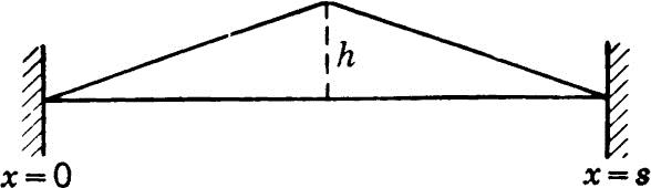
As another example leading to the solution of the wave equation, let us consider the oscillations of a flexible membrane. Let us suppose that the membrane has a density of m g per cm2 and that it is pulled evenly around its edge with a tension of T dynes per cm length of edge. If the membrane is perfectly flexible, this tension will be distributed evenly throughout its area; that is, the material on opposite sides of any line segment dx is pulled apart with a force of Tdx dynes.
Let us call u the displacement of the membrane from its equilibrium position. It is a function of time and of the position on the membrane of the point in question. If we use rectangular coordinates to locate the point, u will’be a function of x, y, and t. Let us consider an element dxdy of the membrane shown in Fig. 8.1.
Fig. 8.1
If we refer to the analogous argument of Sec. 2 for the string, we see that the net force normal to the surface of the membrane due to the pair of tensions Tdy is given by
The net normal force due to the pair Tdx by the same reasoning is
The sum of these forces is the net force on the element and is equal to the mass of the element times its acceleration. That is, we have
Dividing out the common factors of both sides of this equation, we obtain
where
Equation (8.4) is the wave equation for the membrane.
Let us consider the oscillations of the rectangular membrane of Fig. 8.2. Let us assume that
On substituting this assumption into (8.4) and canceling common factors, we obtain
where
Fig. 8.2
Let us now assume
that is, that υ is the product of two functions, a function only of x and the other one only of y. If we substitute this into (8.7), we obtain
This equation may be written in the form
Now the first member of Eq. (8.11) is a function of x only, while the second member is a function of y only. Now a function of y cannot equal a function of x for all values of x and y if both functions really vary with x and y. Thus the only possible way for the equation to be true for both sides to be independent of both x and y is for it to be a constant. Let us call this constant –m2; we then have
We thus obtain the two equations
and
where
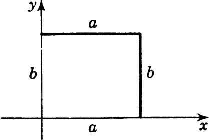
Now since the membrane is fastened at the edges x = 0, x = a, y = 0, y = b, the solution of Eq. (8.13) must vanish at x = 0 and x = a, while the solution of Eq. (8.14) must vanish at y = 0, y = b. A solution of (8.13) that vanishes at 0 is
In order for this to vanish at x = a, we must have
or
A solution of Eq. (8.14) that vanishes at y = 0 is
In order for this solution to vanish at
we must have
Hence
Now from (8.15) we have
Hence the possible angular frequencies are given by
Substituting (8.16) and (8.19) into (8.9), we obtain
Since the indices r and n may take positive integral values and A1 and A2 are arbitrary, we may write instead of (8.25) the function υ (x,y) in the form
If the membrane is excited from rest with an initial displacement u0(x,y) and with no initial velocity, we retain the real part of (8.6) and construct a general solution by summing over all possible values of n and r. We thus obtain
We are now confronted with the question of expanding the function u0(x,y) into the series
Let us first regard y as a constant. In that case u0(x,y) can be expanded in the form
where we have
After the integration with respect to x is performed and the limits substituted, regard An as a function of y and let it be expanded in terms of sin (rπy/b) by the series
where
This determines the arbitrary constants Anr, and the subsequent motion is given by (8.27).
From (8.24) and (8.27) it is evident that if any mode is excited for which n or r is greater than unity we have nodal lines parallel to the edges. It also appears that, if the ratio a2/b2 is not equal to that of two integers, the frequencies are all distinct. However, if a2/b2 is commensurable, some of the periods coincide. The nodal lines may then assume a great variety of forms. The simplest example is the square membrane; in this case we have
for the squares of the angular frequencies.
In the case of the circular membrane we naturally have recourse to polar coordinates with the origin at the center. In this case the equation of motion deduced in Sec. 8 must be transformed from cartesian to polar coordinates. We may write the basic equation of motion of the membrane in the form
where in this case ∇2 is the Laplacian operator in two dimensions. To write this equation in polar coordinates, it is necessary only to write the invariant quantity ∇2u in polar coordinates. Using Eq. (12.20) of Appendix E, we have
Accordingly the wave equation for the membrane becomes in this case
Let us consider the symmetrical case where the motion is started in a symmetrical manner about the origin so that the displacement u is a function only of r and t and independent of the angle θ. This is the case of symmetrical oscillations about the origin. Since in this case we have
Eq. (9.3) becomes
Let us now study the symmetrical oscillations of a circular membrane or radius a that is given an initial displacement u0(r) at t = 0. In this case we have to find a solution of (9.5) that vanishes at r = a and has the initial value u0(r) at t = 0. As in the above examples, let us assume a solution of the form
Substituting this assumed form of the solution in (9.5), we obtain, on dividing out the factor ejωt,
On carrying out the differentiation we have
or
Equation (9.9) is an equation of the form discussed in Appendix B. Its general solution is
where A and B are arbitrary constants and J0 and Y0 are the Bessel functions of the zeroth order and of the first and second kind, respectively. Since the amplitude of the oscillation is finite at the origin, we must have
We must now satisfy the condition that the amplitude of the oscillation must vanish at r = a. Hence we must have
For nontrivial solutions A cannot be equal to zero; hence we must have
From a table of Bessel functions, we find that Eq. (9.14) is satisfied if ka has values 2.404, 5.520, 8.653, 11.791, 14.93, etc. Accordingly the fundamental angular frequency is given by
The other possible angular frequencies are given by the above numbers multiplied by c/a. It is thus seen that there are an infinite number of natural frequencies possible, but these frequencies are not multiples of each other as is the case of the vibrating string. By summing over all the possible values of ω we may construct a general solution of (9.5) that satisfies the boundary condition at the periphery of the membrane and the initial condition that at t = 0 the membrane has no initial velocity and an arbitrary initial displacement u0(r). We thus obtain
Now, at t = 0, we have
Accordingly we must expand an arbitrary function u0(r) in a series of the form
To determine the arbitrary constants An, we may use Eq. (12.20) of Appendix B. We thus obtain
When these values of the constants An are substituted into (9.16), we obtain the subsequent displacement of the membrane.
In this section we shall consider the flow of electricity in a pair of linear conductors such as telephone wires or an electrical transmission line.
Consider a long, imperfectly insulated transmission line, as shown in Fig. 10.1. Let us consider that an electric current is flowing from the source A to the receiving end B in the direction shown in the figure. Let the distance measured along the length of the cable be denoted by x; then both the current i and the potential difference e between the two wires are functions of x and t. Denote the resistance per unit length of the wires by R, the conductance per unit length between the two wires by G, the capacitance per unit length of the two wires by C, and the inductance per unit length by L.
Now consider an element of the transmission line of length Δx. If the electromotive force at the point x is e(x,t), then, if we compute the potential drop along an element of length Δx, we have
However, by Taylor’s expansion, we have
where we neglect terms of higher order. Substituting this into (10.1), we have
Fig. 10.1
If we denote by i(x,t) the current entering a section of length Δx and by i(x + Δx,t) the current leaving this element, we have
where eGΔx is the current that leaks through the insulation and (∂e/∂t)CΔx is the current involved in charging the capacitor formed by the proximity of the two conductors forming the transmission line. By Taylor’s expansion we have
where we neglect higher-order terms. Substituting this into (10.4), we obtain
Equations (10.3) and (10.6) are simultaneous partial differential equations for the potential difference and the current of the transmission line. To eliminate the potential difference, we take the partial derivative of (10.6) with respect to x. We then obtain
We then substitute the value of ∂e/∂x given by (10.3) into (10.7) and thus obtain
In the same manner we have, on eliminating the current,
Equations (10.8) and (10.9) are sometimes known as the telephone equations since they are used in discussing telephonic transmission.
In many applications to telegraph signaling the leakage G is small and the term for the effect of inductance L is negligible, so that we may place
The equations then take the simplified form
These are known as the telegraph, or cable, equations.
For high frequencies the terms in the time derivatives are large, and some qualitative properties of the solution may be found by neglecting the terms for the effect of leakage and resistance in comparison with them. On placing
the equations become
If we let
then we see that in this case both the current and the potential difference between the lines satisfy the one-dimensional wave equation
This equation has the same form as that governing the displacement of the tightly stretched oscillating string. We thus see that a transmission line with negligible resistance and leakage propagates waves of current and potential with a velocity equal to ![]() . The study of Eqs. (10.3) and (10.6) is fundamental in the theory of electrical power transmission and telephony.
. The study of Eqs. (10.3) and (10.6) is fundamental in the theory of electrical power transmission and telephony.
A very interesting special case occurs when the parameters of the transmission line satisfy the relation
The amount of leakage indicated by this equation is reduced by increasing the inductance parameter L. A line having this relation between its parameters is called a distortionless line. This type of line is of considerable importance in telephony and telegraphy.
To analyze this special case, let
Hence
But
Hence Eq. (10.9) in this case becomes
Let us now introduce the variable y(x,t) defined by the equation
If we perform the indicated differentiation and substitute the results into (10.23), we obtain after some reductions
This is a one-dimensional wave equation in y, and its general solution is
where F and G denote arbitrary functions of the arguments x –υt and x + υt, respectively. Now
Hence in view of (10.24) we have
We thus see that the general solution of (10.9) in this case is given by the superposition of two arbitrary waves that travel without distortion to the left and to the right along the line with velocity of υ but with an attenuation given by the factor e–Rt/L.
In most practical power-transmission lines the insulation between the line wires is so good that the leakage conductance coefficient G may be taken equal to zero. In such a case the equations for the potential and current of the transmission line become
To solve (10.30), we let
Making this substitution in (10.30), we obtain after some reductions
Now let
We have
On substituting these expressions for ∂2y/∂x2 and ∂2y/∂t2 in (10.32), we obtain after some reductions
This equation is the modified Bessel differential equation of the zeroth order discussed in Appendix B, Sec. 10. Its general solution is
where I0(z) and K0(z) are modified Bessel functions of the zeroth order of the first and second kind and A and B are arbitrary constants. Since the function K0(z) does not remain finite at z = 0, we must have B = 0. Hence the solution for the current is
The constant A must be determined from a knowledge of the initial conditions of the transmission line.
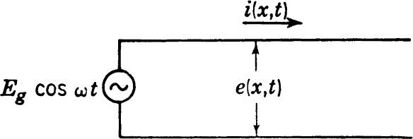
Let us consider the transmission line shown in Fig. 10.2. In this case we consider the effect of impressing a harmonic potential difference of the form
Fig. 10.2
Egcosωt at one end of the line. This case is of great importance in power transmission and in communication networks.
In this case we impress on the line at x = 0 a potential difference of the form
where Re denotes the “real part of.” To solve Eqs. (10.3) and (10.6) in this case, we assume a solution of the form
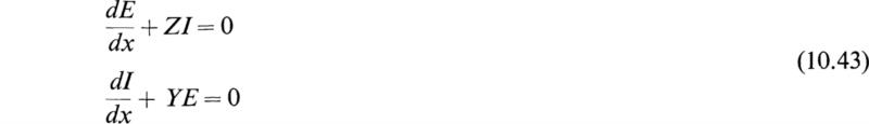
We now substitute these assumed forms of the solution in (10.3) and (10.6) and drop the Re sign, remembering that to get the instantaneous potential difference e(x,t) and the instantaneous current i(x,t) we must use Eqs. (10.40). On substituting the above assumed form of the solution into (10.3) and (10.6) and dividing out the common factor ejωt we obtain
It is convenient to introduce the notation
Then Eqs. (10.41) become
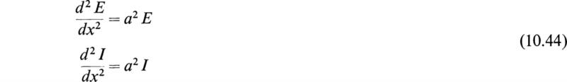
We may eliminate E and I by differentiating each equation with respect to x and substituting either dE/dx or dI/dx from the other. We thus obtain
These equations are linear differential equations of the second order with constant coefficients, and their solutions are
The evaluation of the arbitrary constants A1, A2, B1, B2 requires a knowledge of the terminal conditions of the transmission line. The evaluation of these arbitrary constants in the case of general terminal conditions is straightforward but rather tedious.†
To illustrate the general procedure, let us consider the case of a line short-circuited at x = s, as shown in Fig. 10.3. In this case, we have the boundary conditions
These boundary conditions lead to the two simultaneous equations in the arbitrary constants A1 and A2,
Solving for A1 and A2 and substituting the results into (10.46), we obtain
This result may be written more concisely in terms of hyperbolic functions in the form
Fig. 10.3
We may obtain I(x) directly from (10.43) in the form
If we introduce the notation
then (10.51) may be written in the form
Since a is in general complex, we see that E(x) and I(x) are complex functions of x. To obtain the instantaneous potential e(x,t) and current i(x,t), we must use Eqs. (10.40). An interesting physical significance of the solution may be obtained by considering an indefinitely long line. Since in general a is a complex number, we may write
In this case the arbitrary constant A2 in (10.46) must be equal to zero, since if it were not, the absolute value of E(x) would increase indefinitely. Hence in this case we have
since
![]()
The instantaneous potential is then given by (10.40) in the form
That is, as we travel along the infinite line, the potential is diminished by the factor ![]() and a phase difference a2x is introduced. In this case we have
and a phase difference a2x is introduced. In this case we have
and the instantaneous current is given by (10.40). If there is no dissipation of energy along the line, then R = 0, G = 0; hence
In this case there is no attenuation of potential or current along the line, but we have
This represents a harmonic wave having a phase velocity of ![]() . The current in this case is given by
. The current in this case is given by
The study of more complicated boundary conditions may be undertaken in the same manner, beginning from Eqs. (10.46). An excellent discussion of the general solution will be found in the above-mentioned reference.
Let us consider an incompressible liquid of uniform depth h. The waves which occur on the surface of a liquid may be divided into the following two types:
1. Ripples: These are waves whose wavelength is small, being of the order of ![]() in. These waves owe their propagation to the surface tension in the liquid-air surface and to gravity.
in. These waves owe their propagation to the surface tension in the liquid-air surface and to gravity.
2. Tidal waves: These waves are characterized by having such a long wave-length that the effect of surface tension can be neglected. In the case of these waves the vertical displacement of the surface is small in comparison with the wavelength.
In this section the theory of tidal waves will be discussed. Consider Fig. 11.1. Let the bottom of the liquid be given by the plane y = 0. Let y be
Fig. 11.1
measured so that the y axis points upward. Let the free surface in the xy plane be given by
where h is the depth of the liquid in the undisturbed state and u is the height of the wave above the undisturbed surface of the liquid.
Let the liquid be bounded in the z direction by fixed planes parallel to the xy plane. It will be assumed that these planes are smooth and the liquid slips along them without any frictional resistance.
As a consequence of this assumption the distance between these planes is of no consequence. However, for simplicity, it will be assumed that they are a unit distance apart; that is, the liquid is constrained to move in a uniform canal of unit width and depth h.
Let us use the following notation:
If we neglect the vertical acceleration of the particles of the liquid, we may write the following expression for the pressure at the point x, y:
as a consequence of (11.1).
Now let us consider the vertical strip which is bounded by the planes x and x + dx before the wave motion begins. The volume of this strip is hdx. An instant after the motion is started, let the elevation of the surface of the strip be ys = h + u, and let the planes bounding it have moved to x + υ and x + dx + υ + (∂υ/∂x)dx. The volume of the strip is then (h + u)[dx + (∂v/∂x)dx]. Since the liquid is assumed incompressible, the volume of the strip does not vary with the time. Hence we have
or
where the second term has been neglected since it is a quantity of higher order.
Let the strip under consideration be divided into elements parallel to the bottom. Consider one of these elements of height dy. The force on this element is given by
But from Eq. (11.5) we have
since u is the only function of x in (11.5). Hence the force on the element is given by
The force Fx on the whole strip is obtained by integrating the force on the element of height dy, and we have
This is the rate of increase in momentum by Newton’s second law of motion:
However, differentiating (11.7), we have
Substituting this into (11.12) and dividing by the common factor, we obtain
This is the one-dimensional wave equation discussed in Sec. 3. The velocity of propagation of long waves is therefore
Equation (11.14) may be used to study the pattern of long water waves in a rectangular trough whose length is much greater than its breadth and depth. The conditions at the ends of the trough are υ = 0 at x = 0 and υ = 0 at x = s, where s is the length of the trough.
This analysis is similar to that of the vibrating string of length s considered in Sec. 5. The period of the fundamental oscillation is ![]() . If the restriction that the long waves move only in one dimension is removed, then a similar analysis shows that the quantity υ above satisfies the two-dimensional wave equation.
. If the restriction that the long waves move only in one dimension is removed, then a similar analysis shows that the quantity υ above satisfies the two-dimensional wave equation.
An important class of problems involving wave propagation is that of waves in a compressible fluid such as a gas. The case of sound waves is a particular example of this type of wave motion.
To derive the equation for the propagation of sound in a compressible gas, we recall (see Appendix E) that the general equation of continuity for a fluid is
where ρ is the density of the fluid and v the vector velocity of the fluid defined by
where υx, υy, and υz are the components of the velocity of the fluid in a cartesian frame of reference.
The Euler equation of motion in vector form is
Where p is the pressure of the fluid and F is the “body” force per unit mass.
These fundamental equations will now be applied to the case of wave motion in a perfect gas. The following assumptions will be made:
1. The motion is irrotational so that there exists a velocity potential ϕ defined by the equation
2. The velocities are so small that their squares and products can be neglected.
3. The body force F can be neglected.
Let us write
where ρ0 is the initial value of the density. The quantity s is called the condensation. Since the changes in density in a sound wave are small, the condensation s is small. It will be assumed that as a consequence of this the term ∇·s can be neglected in the continuity equation.
Substituting (12.4) into (12.1), we obtain
By the assumption that s is small this equation becomes
In terms of the velocity potential of Eq. (12.4) this becomes
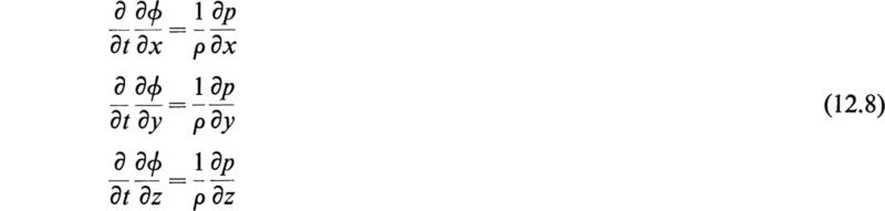
Neglecting the squares and products of the velocities in Eq. (12.3) and writing the resulting vector equation in scalar form, we obtain
If the first equation is multiplied by dx, the second one by dy, the third by dz and the results are added, we obtain
or
Integrating, we obtain
Isaac Newton assumed that the condensation and rarefaction process involved in the propagation of sound waves takes place in such a manner that the temperature of each element of mass is constant. In this case we may assume that Boyle’s law holds, and we have
where ρ is the density, p the pressure, and c a constant. Then we have
by Eq. (12.4a).
Consequently we have
Substituting this into (12.11), we have
Differentiating with respect to t, we obtain
since ![]() .
.
Eliminating ∂s/∂t between (12.16) and (12.7), we have
This isothermal assumption gives the general wave equation (12.17). The velocity of propagation υ0 is
This is the well-known expression derived by Newton for the velocity of sound in a gas. However, it does not agree with experiment since its value is too small.
Laplace showed that, in the case of sound waves, the condensation and rarefaction take place so rapidly that the heat produced has not time to disappear by conduction. Hence the temperature of each element of mass will not be constant, but its quantity of heat will remain constant. This process is not an isothermal one but an adiabatic one.
In this case, instead of Boyle’s law (12.12) we have the adiabatic relation
where c and k are constants. The constant k is given by the following relation:
k is of the order of l.4l for air, oxygen, hydrogen, and nitrogen.
As a consequence of Eqs. (12.19) and (12.4), we have
We also have
Hence by Eq. (12.11)
Since s is small, (1 + s)k–2 ≈ 1 and
as a consequence of (12.19).
Equation (12.23) then may be written in the form
Using (12.7) to eliminate ∂s/∂t, we obtain
and the velocity of propagation of the wave is
This result agrees well with experiment. The velocity of sound in air at standard conditions (20°C, 760 mm Hg) is 34,400 cm per sec.
In this section a very important method of integrating the equations of electrodynamics will be discussed. This method of integration leads to an equation known in the literature as the inhomogeneous wave equation. The integration of this equation is discussed in Sec. 14.
The general equations of electrodynamics, or Maxwell’s equations, are formulated in Appendix E, Sec. 16. They are
The significance of the various symbols is discussed in Appendix E.
In certain problems of electrodynamics the current-density distribution J and the charge density ρ are specified as given functions of space and time. It is then required to determine the electric intensity E and the magnetic intensity H.
In addition to the above equations we have the following relations in a homogeneous isotropic medium:
In order to integrate the Maxwell equations, let us introduce a vector A, defined by the following relation:
The vector A is called the magnetic vector potential.
Substituting (13.8) into (13.1), we obtain
since the order of time differentiation and space differentiation may be interchanged.
Equation (13.9) may be written in the form
This shows that the vector E + ∂A/∂t is irrotational and may therefore be expressed as the gradient of a scalar point function in the form
(ϕ is called the scalar potential) or
If we multiply Eq. (13.2) by μ, we obtain
in view of Eq. (13.6).
by Appendix E, Eq. (11.2). If this result is substituted into (13.13), we have
Equation (13.12) may be differentiated with respect to t, and the result is
The quantity ∂E/∂t may now be eliminated between Eqs. (13.16) and (13.15), and the resulting equation is
or
Now the curl of the magnetic vector potential A is specified by Eq. (13.8). The divergence of A has not been specified.
In order to determine the vector A uniquely, both its curl and its divergence must be specified. Let
Then Eq. (13.18) may be written in the following form:
Equation (13.4) may be written in the form
However, E is given in terms of A and ϕ by Eq. (13.12). Hence, if we substitute this value of E in (13.21), we obtain
or
Eliminate ∇·A between Eqs. (13.19) and (13.23), and we have
Let
Then Eqs. (13.20) and (13.24) may be written in the form
and
These two equations have the same form. In the literature of electrodynamics they are known as the inhomogeneous wave equations, or Lorenz’s equations. The quantity c is the velocity of propagation of electromagnetic waves. If the variation of the current density J and the charge density ρ is given in space and time, then Eqs. (13.26) and (13.27) may be solved for A and ϕ and the field vectors B and E determined by Eqs. (13.8) and (13.12). The solution of Eqs. (13.26) and (13.27) is discussed in the next section.
In the last section it was demonstrated that both the magnetic vector potential A and the scalar potential ϕ are propagated in accordance with equations of the type
This is the inhomogeneous wave equation, or Lorenz’s equation. f(x,y,z,t) is a given function of the space variables and the time t.
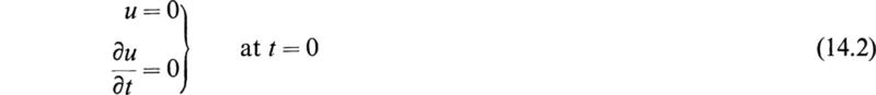
Let it be required to solve this equation subject to the initial conditions
In order to solve this equation, the method of the Laplace transform described in Chap. 4 may be used. Let us introduce the following two transforms,
That is, we introduce a Laplace transform with respect to the time variable. By Theorem (III) of Chap. 4, we have, using (14.2),
Hence, by the Laplace transformation, Eq. (14.1) is transformed to
Let
Then Eq. (14.6) may be written in the form
This equation is known in the literature as Helmholtz’s equation.
Consider the equation
A particular solution of this equation is
where r is the distance from the point where U0 is calculated to another point. By the use of this particular solution the solution of the more general equation (14.8) may be constructed. It is
where x, y,z are the variables of integration and
The fact that (14.11) satisfies (14.8) may be easily verified by differentiation. Let us substitute the value of k given by (14.7) into (14.11). We then obtain
In order to obtain u, the solution of the inhomogeneous wave equation, we must take the inverse transform of U(x,y,z,s) and obtain
To do this, we use Theorem (VII) of Chap. 4. This theorem states that, if Lh(t)= g(s), then
a is a constant. Applying this theorem to (14.13), we obtain
This indicates that the effects in the variation of F(x1,y1,zl,t) do not reach the point x, y, z until a retarded time t – r/c. If the plus sign in the exponential term of (14.13) were used, the inverse transform would lead to an anticipated term of the form t + r/c. These anticipated terms are of little importance in physical applications.
A more complete discussion of the solution of the inhomogeneous wave equation, taking into account more general initial conditions, is given by Pipes.†
Let us return now to the equations governing the propagation of the magnetic vector potential A and the scalar potential ϕ:
and
Comparing these equations with (14.1), we see that they have solutions of the form
and
If the space and time distribution of the current density J and the charge density ρ is known in space and time, then the potentials A and ϕ may be computed. These potentials are called the retarded potentials of electrodynamics. They are of fundamental importance in the theory of electromagnetic waves.
In this section the propagation of electromagnetic waves traveling in the longitudinal direction in a homogeneous isotropic medium that fills the interior of a metal tube of infinite length will be considered. The tube under consideration will be assumed to have a uniform cross section and will be assumed to be straight in the x direction.
It will be assumed that the conductivity of the metal of the tube is infinite. The equations governing the propagation of electromagnetic waves in the interior of tubes are of great importance in the field of communication engineering. †
Let us write the fundamental Maxwell equations in the form
(See Appendix E, Sec. 16.)
These equations govern the distribution of the electric intensity E0 and the magnetic intensity H0 in a medium of conductivity σ, electric inductive capacity K, and magnetic inductive capacity μ. It is assumed that the medium is devoid of free charges.
In order to discuss the possible oscillations that may be propagated inside the waveguide, let us assume that the time dependence of the electric and magnetic fields E0 and H0 is of the form ejωt. Let us take the y and z axes of a cartesian reference frame in the plane of the cross section of the waveguide, and let the x axis be taken in the longitudinal direction along the waveguide.
Let it be assumed that the fields E0 and H0 are of the form
The frequency of the oscillations is f= ω/2π. a is called the propagation constant. E and H are vectors of the form
and
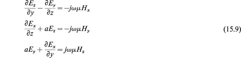
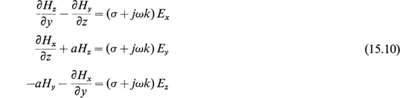
If we substitute Eqs. (15.5) and (15.6) into (15.1) and (15.2) and expand the resulting vector equations into cartesian components, we obtain
It will now be shown that there are two types of waves which satisfy these equations and which may exist independently. In the literature these waves are known as the TM, or E, waves and the TE, or H, waves.
These waves are characterized by the fact that
That is, the electric field has no component in the direction of propagation, and the magnetic field has a component in the direction of propagation.
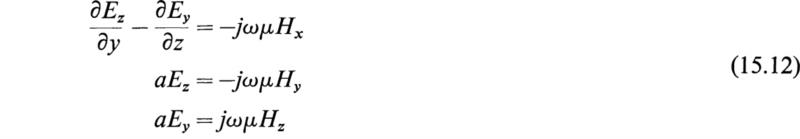
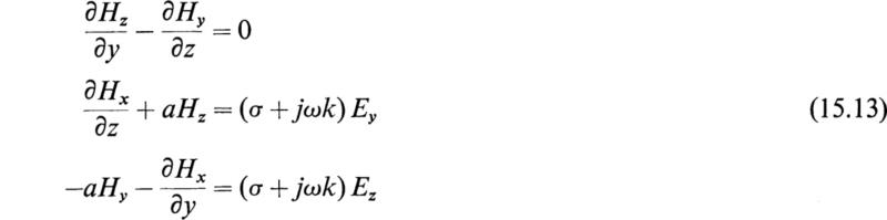
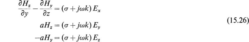
With the restriction that Ex = 0, Eqs. (15.9) and (15.10) become
and
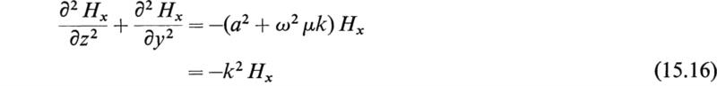
It will be left as an exercise for the reader to show that, if Hy, Hz, Ey, and Ez are eliminated between Eqs. (15.12) and (15.13), the following equation for Hx is obtained:
In dielectric region inside the waveguide we have
Hence (15.14) reduces to
where
Equation (15.16) determines the magnetic intensity Hx subject to the boundary conditions. It may be shown by the use of (15.12) and (15.13) that
This shows that, when Hx is known, then the vector E and the vector H are fully determined.
The boundary conditions If the surface of the metallic waveguide is a perfect conductor, then the tangential component of the E vector must vanish. In the case of a rectangular waveguide whose sides are parallel to the y and z axes we must have Ey and Ez equal to zero at the surface of the waveguide. From Eqs. (15.18) and (15.19) this means that ∂Hx/∂y and ∂Hx/∂z must vanish at the surface.
In the general case the fact that the electric lines of force must enter the perfectly conducting surface σ = ∞ normally implies that
n is the normal to the surface. In general coordinates, Eq. (15.16) may be written in the form
subject to the boundary condition (15.21). It will be noted that this equation has the same form as Eq. (8.7) for the vibrations of a membrane. However, the boundary condition is different.
The solution of Eqs. (15.22) subject to the boundary condition (15.21) determines the possible values of k. For given frequencies, therefore, the values of the propagation constant a are found from the equation
Only imaginary values of a lead to possible wave propagation along the waveguide. If a is real, then the waves are rapidly attenuated as they move along the x direction of the waveguide.
These TM, or E, waves are characterized by the fact that
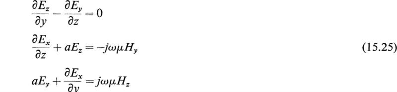
If we place the restriction that Hx = 0 in Eqs. (15.9) and (15.10), we obtain
and
It is possible to eliminate Ez, Ey, Hy, and Hz by the use of these equations and obtain the equation
In the general case, this may be written in the form
The field E can have no tangential component at the surface of the perfectly conducting waveguide. Hence we have the boundary condition
Equation (15.28) and the boundary condition (15.29) are precisely the same as the equation and the boundary condition of the vibrating membrane of Sec. 8. This is the well-known analogy first noticed by Lord Rayleigh. †
The calculation of the possible values of k leads to the possible values of the propagation constant a. The quantities Ez, Ey, Hy, and Hz are determined from Ex by the use of Eqs. (15.25) and (15.26).
1. Find the form at time t of a vibrating string of length s, whose ends are fixed and which is initially displaced into an isosceles triangle. The string is vibrating transversely, is under constant stretching force, and starts from rest.
2. A transversely vibrating string of length s is stretched between two points A and B. The initial displacement of each point of the string is zero, and the initial velocity at a distance x from A is kx(s – x). Find the form of the string at any subsequent time.
3. The differential equation governing the displacement of a viscously damped string is

Find the general solution of this equation when the string has an initial displacement y = y0 (x) and an initial velocity ∂y/∂t = v0(x) at t = 0.
4. A square membrane is made of material of density m g per cm2 and is under a tension of T dynes per cm. What must be the length of one side of the membrane in order that the fundamental frequency be F0 ? What will be the frequencies of the two lowest overtones?
5. A rectangular membrane is struck at its center, starting from rest, in such a way that at t = 0 a small rectangular region about the center may be considered to have a velocity υ0 and the rest has no velocity. Find the amplitudes of the various overtones.
6. Write the differential equation governing the displacement of the general oscillations of a circular membrane. Show that the allowed angular frequencies are determined by the equation

where Jn is the Bessel function of the first kind and nth order, a is the radius of the circular membrane, m the mass per unit area of the membrane, and T the tension per unit length.
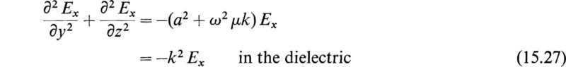
7. Show that the general solution of the differential equations governing the propagation
of current and potential along a dissipationless transmission line R = 0, G = 0 is
Where f and g are arbitrary functions.
These solutions may be interpreted as a combination of two waves, one moving to the left and one moving to the right each with velocity ![]()
8. Show that, if we place G = 0 and L = 0 in the transmission-line equations, we obtain
an equation of the form
![]()
This is the differential equation governing the distribution of temperature in the theory of one-dimensional heat conduction. Discuss the analogy between the transmission line in this case and the one-dimensional heat flow.
9. Show that the small longitudinal oscillations of a long rod satisfy the equation
![]()
where u is the displacement of a point originally at a distance x from the end of the rod, E is the modulus of elasticity of the rod, and m is the density.
10. Find the natural frequencies of vibration of a long prismatic rod of length s, density m, and elastic modulus E, which is fixed at x = 0 and free at x = s.
11. Find the equation that determines the natural frequencies of vibration of the rod described above if the end x = 0 is fixed and the end x = s is fastened to a mass M.
12. Starting with the differential equations of the dissipationless transmission line (R = 0, G = 0) and that governing the oscillations of a long prismatic bar, show that there exists a close analogy between the electrical and mechanical systems. What is the electrical analogue of a long rod oscillating freely whose end at x = 0 is fixed and whose other end at x = s is free ?
13. A string of length l is composed of two separate strings, each of different materials fastened together at the point a. The segment of string from 0 to the point a is one material, and the segment from a to l is the other. Formulate the equations describing this problem, along with the appropriate boundary conditions, and develop the solution in general terms, assuming that the initial position is given by f(x) for 0 < x < l. The string has no initial velocity.
HINT: Assume that the string vibrates as a whole at the same frequency.
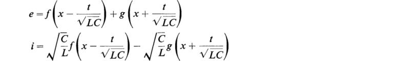
14. Find the solution for the vibrations of a string whose initial velocity is zero and whose initial distribution is
(Kreyszig, 1962)
15. Solve the following partial differential equations by the method of separation of variables:
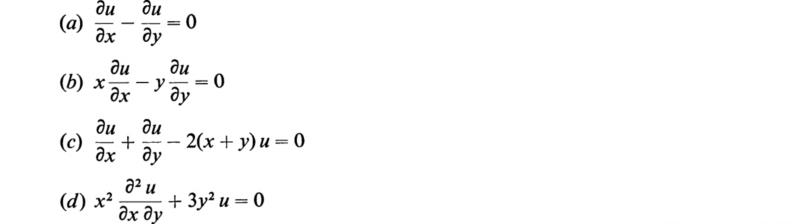
(Kreyszig, 1962)
16. Perform the indicated transformation of the independent variables and solve
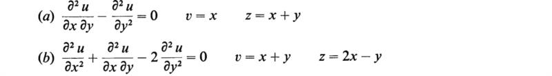
(Kreyszig, 1962)
17. Find the deflection of a unit square membrane if the initial velocity is zero and the initial deflection is

(Kreyszig, 1962)
18. Show that the forced vibrations of an elastic string under an external force P(x,t) per unit length acting normal to the string are governed by the equation
![]()
(Kreyszig, 1962)
1935. Guillemin, E. A.: “Communication Networks,” vol. II, John Wiley & Sons, Inc., New York.
1936. Morse, P. M.: “Vibration and Sound,” McGraw-Hill Book Company, New York.
1937. Timoshenko, S.: “Vibration Problems in Engineering,” D. Van Nostrand Company, Inc., Princeton, N.J.
1962. Kreyszig, E.: “Advanced Engineering Mathematics,” John Wiley & Sons, Inc., New York.
1966. Ostberg, D. R., and F. W. Perkins: “An Introduction to Linear Analysis,” Addison- Wesley Publishing Company, Inc., Reading, Mass.
1966. Raven, F. H.: “Mathematics of Engineering Systems,” McGraw-Hill Book Company, New York.
1966. Sokolnikoff, I. S., and R. M. Redheffer: “Mathematics of Physics and Modern Engineering,” 2d ed., McGraw-Hill Book Company, New York.
1966. Wylie, C. R., Jr.: “Advanced Engineering Mathematics,” 3d ed., McGraw-Hill Book Company, New York.
† See, for example, N. W. McLachlan, “Bessel Functions for Engineers,” Oxford University Press, New York, 1934.
† See, for example, E. A. Guillemin, “Communication Networks,” Chap. 2, John Wiley & Sons, Inc., New York, 1935.
† L. A. Pipes, Operational Solution of the Wave Equation, Philosophical Magazine, ser. 7, no. 26, pp. 333–340, September, 1938.
† See L. J. Chu and W. L. Barrow, Electromagnetic Waves in Hollow Metal Tubes of Rectangular Cross Section, Proceedings of the Institute of Radio Engineers, vol. 26, p. 1520, 1938.
† See Lord Rayleigh, Philosophical Magazine, ser. 5, no. 43, p. 125, 1897.