CHAPTER 10
A 50‐Year Retrospective on Credit Risk Models, the Altman Z‐Score Family of Models, and Their Applications to Financial Markets and Managerial Strategies
THE EVOLUTION OF CORPORATE CREDIT SCORING SYSTEMS
Credit scoring systems for identifying determinants of a firm's repayment likelihood probably go back to the days of the Crusades – when travelers needed “loans” to finance their travels – and certainly were used much later in the United States as companies and entrepreneurs helped to grow the economy, especially in its westward expansion. Primitive financial information was usually evaluated by lending institutions in the 1800s with the primary types of information required being subjective, or qualitative in nature, revolving around ownership and management variables and collateral (see Figure 10.1). It was not until the early 1900s that rating agencies and some more financially oriented corporate entities, for example, the DuPont System of corporate ROE growth, introduced univariate accounting measures and industry peer‐group comparisons, with rating designations (Figure 10.2). The key aspect of these “revolutionary” techniques was the ability of the analyst to compare an individual corporate entity's financial performance metrics to a reference database of time‐series (same entity) and cross‐section (industry) data. Then, and as even more so today, data and databases were the key element for meaningful diagnostics. There is no doubt that in the credit scoring field, data is “king” and models to capture the probability of default ultimately succeed, or not, are based on its ability to be applied to databases of various size and relevance.
|
FIGURE 10.1 Corporate Scoring Systems over Time
The original Altman Z‐Score model (Altman, 1968) was based on a sample of 66 manufacturing companies in two groups, bankrupt and nonbankrupt firms, and a holdout sample of fewer (50) companies. In those “primitive” days, there were no electronic databases and the researcher/analyst had to construct his own database from primary (annual report) or secondary (Moody's and S&P Industrial manuals and reports) sources. To this day, instructors and researchers oftentimes ask me for my original 66‐firm database, mainly for instructional or reference exercises. It is not unheard of today for researchers to have access to databases of thousands, even millions of firms (especially in countries where all firms must file their financial statements in a public database, e.g., in the UK). To illustrate the importance of databases, Moody's, Inc. purchased in 2017 the extensive data on 200 million firms and customer access of Bureau van Dijk Electronic Publishing (EQT) for $3.3 billion and S&P‐purchased SNL's financial institution's extensive database, management structure, and customer‐book for $2.2 billion in 2015. As indicated in Figure 10.2, the three major rating agencies established a hierarchy of creditworthiness that was descriptive, but not quantified, in its depiction of the likelihood of default. The determination of these ratings was based on a combination of (1) financial statement ratio analytics, usually on a univariate, one ratio‐at‐a‐time basis; (2) industry health discussion; and (3) qualitative factors evaluating the firm's management plans and capabilities, strategic directions and other, perhaps “inside‐information,” gleaned from its interviews with senior management and experience of the team that was assigned to the rating decision. To this day, the decision process of rating agencies remains essentially the same with the ultimate rating decision made based on the firm's likelihood of default, and in some cases the loss given default, based on expected recovery. These inputs were analyzed on a “through‐the‐business‐cycle” basis, often based on a “stressed” historical analysis. While the stressed scenario basis for evaluating a firm's solvency is still an important input, rating agencies no longer embrace the business cycle as the key determinant as to whether to change a rating.
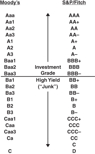
FIGURE 10.2 Major Agencies' Bond Rating Categories
What can we say about this process and its evaluative results? Here are our opinions:
- Since the process has been standardized and carried out fairly consistently over time, it can provide important reference points for the market and is well understood as an “international language of credit.” This makes the database of assigned original ratings and rating changes an incredibly important source of data for both researchers and practitioners on an ongoing basis.
- Original rating assignments are done carefully with adequate resources and a strong desire to assess the repayment potential of the firm on specific issues of bonds, loans, and commercial paper (the so‐called “plain vanilla” issuances of firms) very accurately. The rating assignments do not provide specific quantitative estimates of the probability of default, but do provide important benchmarks for comparing the actual incidence of default on millions of bond issues for long periods of times and to assess the bond‐rating‐equivalent of nonrated firms and securities in order to eventually provide a PD (probability of default) of corporate debt issuances. Hence, we will show this capability in our own “mortality rate” determination based on our original work (Altman 1989) subsequently updated annually, as well as similar analytics introduced by Moody's and S&P in the early 1990s called cumulative default rates and rating transitions tables.1
- We have found, however, that the track record of excellent original rating assignments by the rating agencies is not matched in their performance by the timeliness of rating changes, that is, transitions as the firm's financial and business performance evolves. Studies such as Altman and Rijken (2004) show clearly that agency ratings are generally slower to react to changes, primarily deteriorations in performance, than are established models based on “point‐in‐time” estimations, for example, Z‐Score type models or KMV structural estimates. Indeed, rating agencies openly admit that stability of ratings is a very important attribute of their systems and volatile changes are to be avoided. So, it is no surprise that when rating changes do occur, they are slower than what an objective, unemotional model would produce, and these changes, principally downgrades, are typically smaller (i.e., less notches) than what a model would have produced. The latter implies that if another rating change would follow an initial downgrade, it is highly likely that the second change would be in the same direction as the first – that is, strong autocorrelation of rating downgrades (see Altman and Kao 1992). We have not encountered much, if any, denial from the rating agencies on this observation. After all, the Agencies' clients (firms issuing debt) are more comfortable with a system that provides more stable ratings than one which changes, especially negatively, frequently. And, those using the service, like pension and mutual funds, also prefer stability to volatile ratings.
- These observations illustrate the ongoing discussion and heated arguments as to the objectivity and potential bias of ratings based on the agencies' business model that the same entity that is being rated (firms) also pays for the rating. Critics of rating agencies point to this potential conflict of interest and call for other structures, such as the “investor‐pay” model, or government agencies providing ratings. These have been floated but have not seemed to resonate well with the main protagonist in the rating industry, that is, the users of ratings, primarily investors. And, investors, in some cases, prefer stability of ratings over short‐term volatility, especially if the changes involve a change from investment grade to noninvestment grade, or vice versa. Hence, despite efforts by regulators to encourage alternative systems for estimating PDs, like internally generated or vendor models, ratings from the major rating agencies continue to be an important source of third‐party assessment for the market. We feel that models, like the Altman Z‐Score family, can still play a very important role in the investment process despite the continued prominence of Agency ratings.
Multivariate Accounting/Market Measures
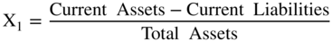
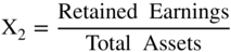
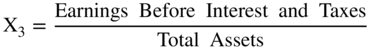
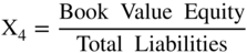
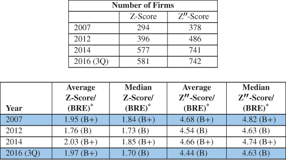
Continuing the evolutionary history of credit scoring beyond univariate systems, (such as those followed by rating agencies and prominent scholarly research studies by numerous academics, such as Beaver 1966) we now move to the first multivariate study to attack the bankruptcy prediction subjects; the initial Z‐Score model. Utilizing one of the first Discriminant Analysis models applied to the economic‐financial social sciences, Altman (1968) and later Deakin (1972), combined traditional financial statement variables with new and more powerful statistical techniques, and aided by early editions of main‐frame computers, constructed the original 1968 Z‐Score model. Consisting of five financial indicators, four of which required only one year of financial statements and one requiring equity market values, the original model (Figure 10.3) demonstrated outstanding original and holdout sample accuracies of Type I (predicting bankruptcy) and Type II (predicting nonbankruptcy) based on a derived cutoff‐score approach (discussed later) and from financial data from one annual statement prior to bankruptcy. The original sample of firms utilized only manufacturing companies, that filed for bankruptcy‐reorganization under the “old” system called Chapter X or XI (now combined under Chapter 11). All firms were publicly held and, given the economic environment in the United States prior to 1966, all had assets under $25 million. The sample sizes were small, only 33 in each grouping, which is remarkable in that the model is still being used extensibly 50 years after its introduction on firms of all sizes, including those with billions of dollars of assets.
| Variable | Definition | Weighting Factor |
| X1 ‐ ‐ ‐ ‐ | 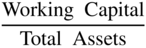 |
1.2 |
| X2 ‐ ‐ ‐ ‐ | 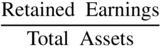 |
1.4 |
| X3 ‐ ‐ ‐ ‐ | 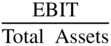 |
3.3 |
| X4 ‐ ‐ ‐ ‐ |  |
0.6 |
| X5 ‐ ‐ ‐ ‐ |  |
1.0 |
FIGURE 10.3 Original Z‐Score Component Definitions and Weightings
The original Z‐Score model was linear and did not require more than one set of financial statements. Subsequent to its introduction, similar models utilizing linear and nonlinear variable structures and different classification techniques, such as quadratic, logit, probit, and hazard model structures were introduced to attempt not only to classify a firm as bankrupt or not, but also to express the outcome in terms of the probability of default based on the characteristics of the sample of firms used in the model's development. An alternative approach for developing PDs, based on the Altman Bond‐Rating Equivalent (BRE) method, combined with empirically derived estimates of default incidence for long horizons (e.g., 1–10 years), will be discussed shortly.
These Discriminant, or Logit, models were applied to consumer credit applications (e.g., Fair Isaac's FICO scores), nonmanufacturers (e.g., ZETA scores; see Altman, Haldeman, and Narayanan (1977), to private firms as well as publicly owned ones, in many other countries (built over several decades and continuing to be derived even in current years), emerging markets (e.g., Altman, Hartzell, and Peck 1995), for internal rating systems (IRBs) of banks (starting in the mid‐1990s and especially since Basel II was first introduced for discussion in 1999) and for various industries and sizes of firms, including models specifically derived for small and medium sized firms (SMEs), for example, Edmister (1972), Altman and Sabato (2007), Altman, Sabato, & Wilson (2010), and, most recently for mini‐bond issuers in Italy, by Altman, Esentato, and Sabato (2016).
Many other exotic statistical and mathematical techniques have been applied to the bankruptcy/default prediction field including expert systems, neural‐networks, genetic algorithms, recursive partitioning, and so on, and the latest attempts using sophisticated machine‐learning methods, motivated by the existence of massive databases and the introduction of nonfinancial data. While these techniques usually surpass the now “primitive” discriminant financial statement based models in terms of prediction‐accuracy tests on original and sometimes holdout samples, the more complex the algorithm and specialized data sources, the less likely that the model will be understood and be able to be replicated by other researchers and by practitioners in its real‐world applications.
One class of model that attained both scholarly and practitioner acceptance and usage is the so‐called structural models built after the introduction of Merton's (1974) contingent‐claims approach for valuing risky‐debt and later the commercialization of the Merton model by KMV's Credit Monitor System. The latter was and still is (marketed by Moody's since 2001) based on a very large sample of defaults derived from companies on a global basis. The result is a PD estimate derived from a distance‐to‐default calculation, relying primarily on firm market values, historical market volatility measures and levels of debt. Academic researchers and several consultants have replicated the Merton‐structural approach and have oftentimes compared it to their own models, as well as more traditional models, like Z‐Scores and Kamakura's reduced‐form approach, see Chava and Jarrow (2004), with results that are not always clear as to which approach was superior; see, for example, Das, Hanouna, and Sarin (2009), Bharath and Shumway (2008), or Campbell, Hilcher, and Szilagi (2008).
The most recent attempts at building both accurate and practically acceptable models have utilized what we call a “blended” Ratio/Market Value/Macro Variable approach, with some attempts to also include nonfinancial variables, where data exists. These blended models, for example, Z‐Metrics (Altman, Rijken, Watt, Balan, Forero, and Mina 2010), introduced by RiskMetrics, are probably the ones that consultants and many financial lenders are either considering or utilizing today, at least in comparison to more traditionally derived models, sometimes with judgmental adjustments by lending officers. And, finally, the FinTech innovations of late are exploring the use of “Big‐Data” and nontraditional metrics, like invoice‐analysis, payable‐history, and governance attributes, “clicks” on negative information events and data,2 and social‐media inputs, in order to capture, on a real‐time basis, changes in credit quality of firms and individuals.
Machine‐Learning Methods
As for machine‐learning and “big‐data” techniques, we remain somewhat skeptical whether many practitioners will accept “black‐box” methods for assessing credit risk of counterparties. Yes, it is undeniable that the current surge in the application of such techniques has captured the interest of many academics and several startups in the FinTech space. Indeed, I collaborated with some colleagues (Barboza, Kumar, and Altman 2017) using several machine‐learning models, for example, support vector machines (SVM), boosting, random forest, and so on, to predict bankruptcy from one year prior to the event and compared the results to discriminant analysis, logistical regression, and neural network methods. Using data from 1985–2013, we found substantial improvement in prediction accuracy (of about 10%) using machine learning techniques, especially when, in addition to the five Z‐Score variables, six additional indicators were included. These results add one more study to the growing debate in the past few years (2014–2017) about the superiority of SVM versus other machine‐learning methods. Almost all of the machine‐learning credit models have been published in expert systems and computational journals, most prominent found in Expert Systems with Applications (see the reference list in Barboza et al., 2017).
FROM A SCORING MODEL TO DEFAULT PREDICTION
The construction of a credit‐scoring model is relatively straightforward with an adequate and appropriate database of default and nondefault securities, or firms, and accurate predictive variables. In the case of our first model, the Z‐Score method (named in association with statistical Z‐measures and also chosen because it is the last letter in the English alphabet), the classification as to whether a corporate entity was “likely” to go bankrupt, or not, was done based on cutoff scores between “Safe” versus “Distress” zones, with an intermediate “Gray” zone (Figure 10.4).


FIGURE 10.4 Zones of Discrimination: Original Z‐Score Model (1968)
These zones were selected based solely on the results of the original, admittedly smallish samples of 33 firms in each of the two groupings (bankrupt and nonbankrupt) from manufacturing firms and their financial statement and equity markets values from the 1960s. Any firm whose Z‐Score was below 1.8 (Distressed Zone) was classified as “bankrupt” and did, in fact, go bankrupt within one year (100% accuracy) and firms whose score was greater than 2.99 did not go bankrupt (also 100% accuracy), at least until the end of the study period in 1966. There were a few errors in classification for firms with scores between 1.81 and 2.99 (Gray Zone – 3 errors out of 66; see Figure 10.5).
| 1969–1975 | 1976–1995 | 1997–1999 | |||
| Year Prior to Failure | Original Sample (33) | Holdout Sample (25) | Predictive Sample (86) | Predictive Sample (110) | Predictive Sample (120) |
| 1 | 94% (88%) | 96% (72%) | 86% (75%) | 85% (78%) | 94% (84%) |
| 2 | 72% | 80% | 68% | 75% | 74% |
| 3 | 48% | – | – | – | – |
| 4 | 29% | – | – | – | – |
| 5 | 36% | – | – | – | – |
FIGURE 10.5 Classification and Prediction Accuracy Z‐Score (1968) Failure Model*
*Using 2.67 as cutoff (1.81 cutoff accuracy in parenthesis).
Keep in mind that these cutoff‐scores were based solely on the original sample of firms. But, because the zones were clear, unambiguous and consistently accurate in their subsequent predictions of greater than 85%, based on data from one year prior to bankruptcy (Type I) (Figure 10.5), these designations remain to this day as accepted and useful to market practitioners. While flattering to this writer, this is unfortunate as it is obvious that the dynamics and trends in credit‐worthiness have changed significantly over the past 50 years. And, the classification as to “Bankrupt” or “Nonbankrupt” is no longer sufficient for many applications of the Z‐Score model. Indeed, there is very little difference between a firm whose score is 1.81 versus one whose score is 1.79, yet, the zones are different. In addition, certainly the “holy grail” in credit assessment, namely the probability of default (PD) and when the default associated with the probability is to take place, are not specified clearly by a certain credit score. We now examine how credit dynamics have changed over our relevant time periods and how have we moved on to precise PD and timing of default estimates.
Time‐Series Impact on Corporate Z‐Scores
When we built the original Z‐Score model in the mid‐1960s, financial credit markets were much simpler, some might say primitive, compared to today's highly complex, multistructured environment. Such innovations as high‐yield bonds, leverage‐loans, structured financial products, credit derivatives, such as CDS (credit default swaps), and “shadow‐banking” loans were nonexistent then, and riskier companies had little financing alternatives outside of traditional bank loans and trade‐debt. For example, we see from Figure 10.6 that the North American high‐yield bond market had not been “discovered” until the late 1970s when the only participants were the so‐called “fallen‐angel” companies that raised debt originally when they were investment grade (IG). In 2017, the size of the high‐yield “junk‐bond” market has grown from about $10 billion of fallen angels in 1978 to about $1.7 trillion, with over 85% of this market consisting of “original‐issue” high‐yield issues. In addition, the pace of newly issued high‐yield bonds and leverage‐loans, has accelerated since the great financial crisis (GFC) of 2008/2009, with more than $200 billion of new bond issues each year since 2010, fueled by a benign credit‐cycle, which has continued now into its ninth year in 2018. Not to be outdone, loans to noninvestment grade companies have again become numerous and available at attractive rates as interest rates have fallen, in general, and banks, despite regulatory oversight guidelines (e.g., Debt/EBITDA ratios not to exceed a certain level, e.g., 6), have competed with the public markets in the United States and Europe. These leveraged loans' new issues of several hundred billions per year ($651 billion in 2017 in the United States alone) have swelled corporate debt ratios to an unprecedented level as firms have exploited the easy‐money, low‐interest‐rate environment and lenders seek yield, even for the most risky corporate entities. For example, CCC new issues have averaged 15.0% of all high‐yield bond new issues over the period 2010–2017 (2Q).
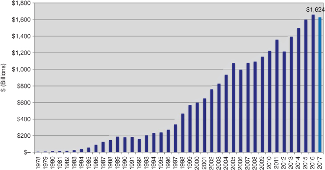
FIGURE 10.6 Size of the U.S. High‐Yield Bond Market 1978–2017 (Mid‐year US$ Billions)
Source: NYU Salomon Center estimates using Credit Suisse, S&P, and Chili data.
Other factors that have reduced the average credit‐worthiness of companies as the Z‐Score model has matured in the 50‐year period since its inception are global competitive factors, the enormous power of market dominating firms in certain industries, such as Walmart and Amazon in the retail space, and the amazing susceptibility of larger companies to financial distress and bankruptcy. Indeed, when we built the Z‐Score model in the 1960s, the largest bankrupt firm in our sample had total assets of less than $25 million (about $125 million, inflation adjusted) compared to an environment with a median annual number of 14 firms each year since 1990 with liabilities (and assets) of more than $1 billion.
To demonstrate the implied deterioration in corporate creditworthiness over the past 50 years, one can observe our median Z‐Score statistics by S&P credit rating for various sample years shown in Figure 10.7. First, the number of AAA ratings has dwindled to just two in 2017 (Microsoft and Johnson & Johnson) from 15–20 years ago and 98 in 1992! Hence, we now combine AAA‐ and AA‐rated companies to analyze average Z‐Scores and that median has decreased from a high of 5.20 in the 1996–2001 period to 4.30 in 2017. Of even more importance, is the steady deterioration of median Z‐Scores for single‐B companies from 1.87 in 1992–1995 to 1.65 in 2017. Recall that a score of below 1.8 in 1966 was classified as a firm in the Distress Zone and a strong bankruptcy prediction. However, in the past 15 years, or so, the dominant and largest percentage of issuance in the high‐yield market was single‐B, and surely all single‐Bs do not default! Yes, a median single‐B has a distribution with 50% of the issues higher than 1.65, but the probability of all Bs that default within five years of issuance is approximately “only” 28% (see our mortality‐rate discussion shortly). Finally, the median “D” (Default‐rated company) had a Z‐Score of –0.10 in 2017, while the median Z‐Score in 1966 for bankruptcy entities was +0.65 (see Altman 1968 or Altman and Hotchkiss 2006). In all time periods of late, the median defaulted firm's Z‐Score was zero or below (Figure 10.7). Hence, we suggest that a score below zero is consistent with a “Defaulted” company. The cutoff of 1.8, based on our original sample, will place an increasing number, perhaps as much as 25% of all firms, in the old “Distress” zone. Since only a very small percentage of all firms fail each year and an average of about 3.5% of high‐yield bond companies default each year, based on data over the last almost 50 years (see our default rate calculations, in Altman & Kuehne 2017 and Chapter 9 herein), the so‐called Type II error (predicting default when the firm does not) has increased from about 5% in our original analysis to possibly 25–30% in recent periods. Hence, we do not recommend that users of our Z‐Score model make their assessments of a firm's default likelihood based on a cutoff score of 1.8. Instead, we recommend using bond‐rating‐equivalents (BREs), based on the most recent median Z‐Scores by bond‐rating, such as the data listed in Figure 10.7. These BREs can then be converted into more granular PD estimates, as we now discuss.
| Rating | 2017 (No.) | 2013 (No.) | 2004–2010 | 1996–2001 | 1992–1995 |
| AAA/AA | 4.30 (14) | 4.13 (15) | 4.18 | 5.20 | 5.80* |
| A | 4.01 (47) | 4.00 (64) | 3.71 | 4.22 | 3.87 |
| BBB | 3.17 (120) | 3.01 (131) | 3.26 | 3.74 | 2.75 |
| BB | 2.48 (136) | 2.69 (119) | 2.48 | 2.81 | 2.25 |
| B | 1.65 (79) | 1.66 (80) | 1.74 | 1.80 | 1.87 |
| CCC/CC | 0.90 (6) | 0.33 (3) | 0.46 | 0.33 | 0.40 |
| D | −0.10 (9)1 | 0.01 (33)2 | −0.04 | −0.20 | 0.05 |
* AAA Only; No. = Number of firms in the sample.
1 From 1/2014 to 11/2017;
2 From 1/2011 to 12/2013.
FIGURE 10.7 Median Z‐Score by S&P Bond Rating for U.S. Manufacturing Firms, 1992–2017
Source: Compustat database, mainly S&P 500 firms, compilation by E. Altman, NYU Salomon Center, Stern School of Business.
PD Estimation Methods
Figure 10.8 lists two methods we have used over the years to estimate the probability of default and loss‐given‐default of a firm's bond issue at any point in time. The starting point in both methods, is a well‐constructed and, if possible, intuitively understandable credit‐scoring model. For example, the Z‐Score on a new, or existing, debt issuer is then, in Method #1, assigned a Bond‐Rating‐Equivalent (BRE) on a representative sample of bond issues for each of the major rating categories (seeFigure 10.7) or, if available, more granular ratings with (+) or (–) “notches (S&P/Fitch) or 1, 2, 3 (Moody's). See Figure 10.15, at a later point, for the more granular categorization for another of the Altman Z‐Score models, Z″‐Scores.
In addition to the matching of Z‐Scores by rating category, we also can assess the PD of an issue for various periods of time in the future. The more traditional time‐dependent method is called “Cumulative Default Rates” (CDRs) as provided by all of the rating agencies and by several of the investment banks who provide continuous research on defaults, particularly for the speculative grade, or high‐yield (“junk bond”) market. This compilation, is an empirically derived PD estimate of bonds with a certain rating, for example, “B”, at a point in time, and then the default incidence is observed 1, 2, … 10 years, after that point in time. The estimate is for all B– rated bonds regardless of the age of the bond when it is first tracked. In our opinion, this PD estimate is more appropriate for existing bond issuer's debt, not for bonds when they are first issued. Almost all of the rating agencies, with the exception of FITCH, Inc., calculate the CDRs based on the number of issuers that default over time compared to the number of issuers with a certain rating at the starting point (regardless of the different ages of the bonds in the “basket” of, say, B‐rated bonds). Therefore, on average, an S&P B‐rated bond had about a 5% incidence of default within one year based on a sample of bonds from 1980–2016 (see Standard & Poor's, 2017).
| Method #1 |
|
| Or |
| Method #2 |
|
FIGURE 10.8 Estimating Probability of Default (PD) and Probability of Loss Given Defaults (LGD)
Before the rating agencies first compiled their cumulative default rates, Altman (1989) created the “mortality rate” approach for estimating PDs for bonds of all ratings and specifically for newly issued bonds and based on dollar amounts of new issues‐by‐bond‐rating, not by issuers. These mortality estimates are based on insurance‐actuarial techniques to calculate the marginal and cumulative mortality rate, as shown in Figure 10.9. I felt, just like “people‐mortality,” there are certain characteristics of bonds, or loans, at birth that are critical in determining the likelihood of default over up to 10 years after issuance (the usual maturity of newly issued bonds). In addition, those characteristics can be summarized into an issue's (not an issuer's) bond rating at birth. Implicit in these PD estimates is the aging‐effect of a bond issue, whereby the first year's mortality rate after issuance is relatively low compared to the second year; similarly, the second is usually lower than the third year's marginal rate, as shown in Figure 10.10. Note that the mortality rates in Figure 10.10 are based on the incidence of defaults for the 46‐year period, 1971–2016. For example, the marginal default (or mortality) rate of a BB‐rated issue for years 1, 2, and 3 after issuance is 0.92%, 2.04%, and 3.85% respectively. After three years, marginal rates seem to flatten out at between 1.5 and 2.5% per year.

| MMR | = | marginal mortality rate |
One can measure the cumulative mortality rate (CMR) over a specific time period (1, 2,…, T years) by subtracting the product of the surviving populations of each of the previous years from one (1.0), that is,
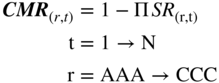
here
| CMR(r,t) | = | Cumulative Mortality Rate of (r) in(t), |
| SR(r,t) | = | Survival Rate in(r,t), 1 – MMR(r,t) |
FIGURE 10.9 Marginal and Cumulative Mortality Rate Actuarial Approach
| Years After Issuance | |||||||||||
| 1 | 2 | 3 | 4 | 5 | 6 | 7 | 8 | 9 | 10 | ||
| AAA | Marginal | 0.00% | 0.00% | 0.00% | 0.00% | 0.01% | 0.02% | 0.01% | 0.00% | 0.00% | 0.00% |
| Cumulative | 0.00% | 0.00% | 0.00% | 0.00% | 0.01% | 0.03% | 0.04% | 0.04% | 0.04% | 0.04% | |
| AA | Marginal | 0.00% | 0.00% | 0.19% | 0.05% | 0.02% | 0.01% | 0.01% | 0.01% | 0.01% | 0.01% |
| Cumulative | 0.00% | 0.00% | 0.19% | 0.24% | 0.26% | 0.27% | 0.28% | 0.29% | 0.30% | 0.31% | |
| A | Marginal | 0.01% | 0.03% | 0.10% | 0.11% | 0.08% | 0.04% | 0.02% | 0.23% | 0.06% | 0.03% |
| Cumulative | 0.01% | 0.04% | 0.14% | 0.25% | 0.33% | 0.37% | 0.39% | 0.62% | 0.68% | 0.71% | |
| BBB | Marginal | 0.31% | 2.34% | 1.23% | 0.97% | 0.48% | 0.21% | 0.24% | 0.15% | 0.16% | 0.32% |
| Cumulative | 0.31% | 2.64% | 3.84% | 4.77% | 5.23% | 5.43% | 5.66% | 5.80% | 5.95% | 6.25% | |
| BB | Marginal | 0.91% | 2.03% | 3.83% | 1.96% | 2.40% | 1.54% | 1.43% | 1.08% | 1.40% | 3.09% |
| Cumulative | 0.91% | 2.92% | 6.64% | 8.47% | 10.67% | 12.04% | 13.30% | 14.24% | 15.44% | 18.05% | |
| B | Marginal | 2.85% | 7.65% | 7.72% | 7.74% | 5.72% | 4.45% | 3.60% | 2.04% | 1.71% | 0.73% |
| Cumulative | 2.85% | 10.28% | 17.21% | 23.62% | 27.99% | 31.19% | 33.67% | 35.02% | 36.13% | 36.60% | |
| CCC | Marginal | 8.09% | 12.40% | 17.71% | 16.22% | 4.88% | 11.60% | 5.39% | 4.73% | 0.62% | 4.23% |
| Cumulative | 8.09% | 19.49% | 33.75% | 44.49% | 47.20% | 53.33% | 55.84% | 57.93% | 58.19% | 59.96% | |
* Rated by S&P at issuance.
Based on 3,359 issues.
FIGURE 10.10 Mortality Rates by Original Rating, All Rated Corporate Bonds,* 1971–2017
Source: Standard & Poor's (New York) and author's compilation.
Method #1's PD estimate is derived from Figure 10.9's equations and when adjusted for recoveries on the defaulted issue, we can derive estimates for Loss‐Given‐Default in Figure 10.11. This critical LGD estimate can be utilized to estimate expected losses in a bank's Basel II or III capital requirements, or for an investor's expected loss on a portfolio of bonds categorized by bond rating. (See our discussion of lender applications later from Figure 10.17). The earliest measures of LGD that I am aware of were from Altman (1977) and Altman Haldeman, and Narayanan (1977).
| 1 | 2 | 3 | 4 | 5 | 6 | 7 | 8 | 9 | 10 | ||
| AAA | Marginal | 0.00% | 0.00% | 0.00% | 0.00% | 0.01% | 0.01% | 0.01% | 0.00% | 0.00% | 0.00% |
| Cumulative | 0.00% | 0.00% | 0.00% | 0.00% | 0.01% | 0.02% | 0.03% | 0.03% | 0.03% | 0.03% | |
| AA | Marginal | 0.00% | 0.00% | 0.02% | 0.02% | 0.01% | 0.01% | 0.00% | 0.01% | 0.01% | 0.01% |
| Cumulative | 0.00% | 0.00% | 0.02% | 0.04% | 0.05% | 0.06% | 0.06% | 0.07% | 0.08% | 0.09% | |
| A | Marginal | 0.00% | 0.01% | 0.04% | 0.04% | 0.05% | 0.04% | 0.02% | 0.01% | 0.05% | 0.02% |
| Cumulative | 0.00% | 0.01% | 0.05% | 0.09% | 0.14% | 0.18% | 0.20% | 0.21% | 0.26% | 0.28% | |
| BBB | Marginal | 0.22% | 1.51% | 0.70% | 0.57% | 0.25% | 0.15% | 0.09% | 0.08% | 0.09% | 0.17% |
| Cumulative | 0.22% | 1.73% | 2.41% | 2.97% | 3.21% | 3.36% | 3.45% | 3.52% | 3.61% | 3.77% | |
| BB | Marginal | 0.54% | 1.16% | 2.28% | 1.10% | 1.37% | 0.74% | 0.77% | 0.47% | 0.72% | 1.07% |
| Cumulative | 0.54% | 1.69% | 3.94% | 4.99% | 6.29% | 6.99% | 7.70% | 8.14% | 8.80% | 9.77% | |
| B | Marginal | 1.90% | 5.36% | 5.30% | 5.19% | 3.77% | 2.43% | 2.33% | 1.11% | 0.90% | 0.52% |
| Cumulative | 1.90% | 7.16% | 12.08% | 16.64% | 19.78% | 21.73% | 23.56% | 24.41% | 25.09% | 25.48% | |
| CCC | Marginal | 5.35% | 8.67% | 12.48% | 11.43% | 3.40% | 8.60% | 2.30% | 3.32% | 0.38% | 2.69% |
| Cumulative | 5.35% | 13.56% | 24.34% | 32.99% | 35.27% | 40.84% | 42.20% | 44.12% | 44.33% | 45.83% |
* Rated by S&P at issuance.
Based on 2,797 issues.
FIGURE 10.11 Mortality Losses by Original Rating, All Rated Corporate Bonds,* 1971–2017
Source: Standard & Poor's (New York) and author's compilation.
Method #2 utilizes a different approach to estimate PDs. Instead of using empirical estimates of defaults by bond rating, companies are analyzed with a logistic regression methodology, whereby the company is assigned a “0” or “1” dependent variable based on whether it defaulted or not at a specific point in time, and then a number of independent, explanatory variables are analyzed in the regression format to arrive at a PD estimate between 0 and 1.3 The resulting PDs are then assigned a rating‐equivalent based on, for example, the percentage of bond issues that are AAA, AA, A … CCC, in the “real world.” This logistic structure is used widely in the academic literature and has been a standard technique ever since the early work of Ohlson (1980). We (e.g., Altman et al. [2010], Z‐Metrics) have also used it for our hybrid‐model estimations.
Which is the superior technique for estimating PD, Methods #1 or #2? I favor the BRE approach for newly issued debt (mortality rate approach) but for existing issues, the cumulative default rate method seems to be more appropriate. The reasons are that the mapping of PDs to BREs using mortality rates, or CDRs, are based on over one million issues and about 3,500 defaults over the past 45 years. Logistical regression models' PDs are a function of the sample characteristics used to build the model and the results are based on the logistic structure, which may not be representative of large sample properties. The beauty of logistical regression estimates, however, is that the analyst can access PDs directly from the results and avoid the mapping of scores as an intermediate step. Test of Types I and II accuracies are available for both methods, as well as statistical AUC (area under the curve) accuracy measures on both original and holdout samples. The latter is very important to help validate the empirical results from samples over time and from different industrial groups. From our experience, both methods have yielded very impressive Type I accuracies in numerous empirical tests.
Z‐Score Model for Industrials and Private Firms
As noted earlier, the original 1968 Z‐Score model was based on a sample of manufacturing, publicly held firms whose asset and liability size was no greater than $25 million. The fact that this model has retained its high Type I accuracy on subsequent samples of manufacturing firms (Figure 10.5) and is still to this date extensively used by analysts and scholars, even for nonmanufacturers, is quite surprising given that it was developed 50 years ago. It is evident, however, that nonmanufacturing firms, like retailers and service firms, have very different asset and liabilities structures and income statement relationships with asset levels, like the Sales/Total Assets ratio, which is considerably greater on average for retail companies than manufacturers, perhaps twice as high. And, given the 1.0 weighting for the variable (X5) in the Z‐model (Figure 10.3), most retail companies have a higher Z‐Score than manufacturers. For example, even the beleaguered Sears Roebuck & Co. latest Z‐Score (Figure 10.12) in 2016 was 1.3, a BRE of B–, compared to a “D” rating equivalent using the Z″‐Score (discussed next); the latter model does not contain the Sales/Total Asset ratio and was developed for a broad cross‐section of industrial sector firms, as well as for firms outside the United States (see Altman, Hartzell, and Peck 1995).
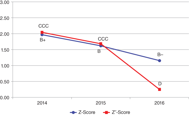
FIGURE 10.12 Z and Z″‐Score Models Applied to Sears, Roebuck & Co.: Bond Rating Equivalents and Scores from 2014 to 2016
Source: S&P Capital IQ and NYU Salomon Center calculations.
To adjust for the industrial sector impact, we have built “second‐generation” models for a more diverse industrial grouping, for example, the ZETA model (Altman, Haldeman, and Narayanan 1977) and for firms in emerging markets, (Altman, Hartzell, and Peck 1995). Additional Altman Z‐Score models developed over the past 50 years for various organizational structured firms, for example, private firms (Z′), developed at the same time (1968) as the original Z‐model; textile firms in France (Altman, Margaine, Schlosser, and Vernimmen 1974); industrials in the United States (ZETA, Altman et al. 1977); Brasil (Altman, Baidya, and Riberio‐Dias 1979); Canada (Altman and Lavallee 1981); Australia (Altman and Izan 1982); China (Altman, Zhang, and Yen 2010); South Korea (Altman, Eom, and Kim 1995); non‐US, Emerging Market (Z″) firms (Altman, Hartzell, and Peck 1995); SME models for the United States (Altman and Sabato 2007) and the UK (Altman, Sabato, and Wilson 2010); Italian SMEs and Minibonds (Altman, Esentato, and Sabato 2016); and for Sovereign Default Risk Assessment (Altman and Rijken 2011).
Private Firm Models
It has been most convenient to build credit‐scoring models for publicly owned, listed companies in the United States and abroad due to data availability. Models for private firms can be built, indirectly, by using only those variables related to private firms, but based on publicly owned firm data, or by accessing databases which are populated by both publicly owned and private companies. The latter is especially available in several European countries via tax reporting and government Credit Bureau sources, for example, the UK, firm private databases, for example, from Bureau van Dijk (now owned by Moody's).
I used the indirect method in the Z′‐Score models, discussed in (Altman 1983) and shown in Figure 10.13. The only difference from the original Z‐Score model is the substitution of the book value of equity for the market value in X4. Note that all of the coefficients are now different, but only slightly so, and the zones (Safe, Gray, and Distress) were slightly different, as well. There was some slight loss in accuracy by this model adjustment, but over the years this “private‐firm‐model” has retained its accuracy based on applications to individual private firm bankruptcies. These results have never been published, however.
 |
 |
 |
 |
 |
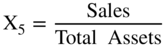 |
FIGURE 10.13 Z‐Score Private Firm Model
Source: Author's calculations.
I have also built numerous models for firms in non‐U.S. countries generally following the pattern of first trying the original model on a sample of local firm bankrupts and nonbankrupts and then adding or subtracting variables thought to be helpful in those countries for more accurate prediction. In some cases, different criteria for the distressed‐firm sample had to be used due to the lack of formal bankruptcies. An example was our China model (Altman, Zhang, and Yen 2010) which utilized firms classified as ST (Special Treatment) due to their consistent losses and book‐equity dropping below par value. In others, such as in Australia (Altman and Izan 1982), the explanatory variables were all adjusted for industry‐averages so that the model was thought to be more appropriate and accurate across a wide spectrum of industrial sectors. In the case of the sovereign risk assessment model (Altman and Rijken 2011), in addition to traditional financial ratios and market value levels and volatility measures, the authors added macroeconomic variables, such as yield spreads and inflation indicators, in their Z‐Metrics model applied to all nonfinancial, listed firms in order to assess the sovereign's private sector health. This modeling approach is applicable to any country in the world as long as data on listed or nonlisted private sector companies is available. See the discussion at a later point on the sovereign risk application, following Figure 10.17.
The Z”‐score Model
As noted in Figure 10.14, we built a model (Z″‐Score) for all industrial, manufacturing and nonmanufacturers in 1995 and first applied it to Mexican companies and then to other Latin American firms. It has since been successfully applied in the United States and in just about any other country, usually with superior accuracy compared to the original Z‐Score model when the data includes nonmanufacturers. This Z″‐Score model is also applicable to privately owned firms since X4 is denominated in book equity to total liabilities, not market values. This substitution is particularly important for environments where the stock market is not considered a good valuation measure due to its size, scope, liquidity, or trading factors. In addition, note that the original fifth variable, Sales/Total Assets, is no longer in this model. We found that the X5 variable was particularly sensitive to industrial sectors differences, for example retail or service firms versus manufacturing companies, and in countries whereby capital for investment in fixed assets was inadequate. Finally, this version of the Altman family of models that used Discriminant Analysis also has a constant term (3.25). The constant standardized the results such that scores slightly above or below zero are in the D‐rated BRE (see Figure 10.15 for BREs more granular than the major rating categories). The Type I accuracy of the Z″‐Score model over time is shown in Figure 10.16.
 |
 |
 |
 |
 |
FIGURE 10.14 Z″‐Score Model for Manufacturers, Nonmanufacturer Industrials; Developed and Emerging Market Credits (1995)
Source: Author's calculations from Altman, Hartzell and Peck (1995).
 |
|||
| Rating | Median 1996 Z″‐Scorea | Median 2006 Z″‐Scorea | Median 2013 Z″‐Scorea |
| AAA/AA+ | 8.15 (8) | 7.51 (14) | 8.80 (15) |
| AA/AA– | 7.16 (33) | 7.78 (20) | 8.40 (17) |
| A+ | 6.85 (24) | 7.76 (26) | 8.22 (23) |
| A | 6.65 (42) | 7.53 (61) | 6.94 (48) |
| A– | 6.40 (38) | 7.10 (65) | 6.12 (52) |
| BBB+ | 6.25 (38) | 6.47 (74) | 5.80 (70) |
| BBB | 5.85 (59) | 6.41 (99) | 5.75 (127) |
| BBB− | 5.65 (52) | 6.36 (76) | 5.70 (96) |
| BB+ | 5.25 (34) | 6.25 (68) | 5.65 (71) |
| BB | 4.95 (25) | 6.17 (114) | 5.52 (100) |
| BB− | 4.75 (65) | 5.65 (173) | 5.07 (121) |
| B+ | 4.50 (78) | 5.05 (164) | 4.81 (93) |
| B | 4.15 (115) | 4.29 (139) | 4.03 (100) |
| B– | 3.75 (95) | 3.68 (62) | 3.74 (37) |
| CCC+ | 3.20 (23) | 2.98 (16) | 2.84 (13) |
| CCC | 2.50 (10) | 2.20 (8) | 2.57(3) |
| CCC– | 1.75 (6) | 1.62 (–)b | 1.72 (–)b |
| CC/D | 0 (14) | 0.84 (120) | 0.05 (94)c |
a Sample size in parentheses.
b Interpolated between CCC and CC/D.
c Based on 94 Chapter 11 bankruptcy filings, 2010–2013.
FIGURE 10.15 U.S. Bond Rating Equivalents Based on Z″‐Score Model
Source: Author calculations based on data from S&P Global.
| Number of Months Prior to Bankruptcy Filing | Original Sample (33) | Holdout Sample (25) | 2011–2014 Predictive Sample (69) |
| 6 | 94% | 96% | 93% |
| 18 | 72% | 80% | 87% |
FIGURE 10.16 Classification and Prediction Accuracy (Type I) Z‐Score Bankruptcy Model*
*E. Altman and J. Hartzell, “Emerging Market Corporate Bonds: A Scoring System,” Salomon Brothers Corporate Bond Research, May 15, 1995, Summarized in E. Altman and E. Hotchkiss, Corporate Financial Distress and Bankruptcy, third ed. (Hoboken, NJ: Wiley, 2006).
SCHOLARLY IMPACT
Perhaps because of its simplicity, transparency and consistent accuracy over the years, the Z‐Score models have been referenced and compared to in a large number of academic and practitioner studies in finance and accounting over the years. These references and comparisons have taken at least three forms. The first is to construct alternative models and frameworks to predict bankruptcy or defaults. The original model and its success, using a combination of financial and market valuation data with robust statistical analysis, made the task of default risk assessment more attractive for scientific work in many disciplines. It opened the door not only for finance and accounting scholars, but also statisticians and mathematicians, to find better and more efficient indexes and to examine new indicators and techniques, especially as expanded and more easily accessible databases became available.
New frameworks have involved seemingly more powerful statistical and mathematical techniques, such as logit, probit, or, quadratic nonlinear regressions, or artificial intelligence, neural networks, genetic algorithms, recursive partitioning, machine‐learning, and structural, distance‐to‐default or hazard models, among others. Since the Z‐score model was easily replicable, it usually was chosen by researchers to be compared in terms of accuracy of classification and prediction. These studies are too numerous to list individually, but probably number in the hundreds, including several by this author with numerous co‐authors (see References).4 The combination of simple, but theoretically well grounded, empirical analysis provided new and attractive avenues in bankruptcy research, laying the foundation for expanded modern understanding of bankruptcy prediction, see Scott (1981). For example, recent studies (Altman, Iwanicz‐Drozdowska, Laitinen, and Suvas 2016; 2017) looked at several dimensions of bankruptcy prediction research for (a) long distance (10 years) time‐series accuracy (Duffie, Saita, and Wang 2007), (b) a number (5) of different statistical techniques, and (c) numerous (34) different country databases and environments. Results covering 31 European countries and three others (China, Colombia, and the United States), showed that while models built specifically for individual countries usually outperformed the original Z‐models, the added‐value of new country‐specific variables and data and numerous frameworks was not dramatic. Despite somewhat higher accuracies using the Z″‐Score variables on data specific to each country, we found that the original weightings continued to show remarkable performance despite their determination more than two decades earlier.
Studies using accounting data, among other variables, potentially suffer when the data is either not very reliable, for example, from emerging markets, or is subject to earnings management manipulations. A recent study by Cho, Fu, and Yu (2012), reconstructed Z‐Scores for this manipulation with the resulting accuracy improved.
The second dimension of Z‐Score's scholarly impact is in its international “reach.” Since the original model and its derivatives (e.g., Z″‐Score) has stood the test of time, it has been widely applied in multiple settings, including application across all domains, with its sharp focus on a few key variables. Also important, is its robust empirical stability over long periods of time and its global applicability and understandability. We are familiar with Z‐Score type models built and tested in at least 30 different countries, based on at least 70 individual articles, and even more in studies analyzing at least that many countries in a single study. Indeed, I helped assemble two special journal issues devoted to a large number of specific country models, see Altman (editor), 1984b and 1988. Those studies, and more, are also listed and described in Altman and Hotchkiss (2006).. More recent studies can also be found in our earlier discussion on scholarly impact and in Choi (1997).
The third impact dimension is related to corporate financial management, especially the important subject of optimal capital structure and the tradeoff between the tax advantage of debt financing and expected bankruptcy and other distress costs. My contribution to this question (Altman 1984a), discussed and measured empirically, for the first time, the so‐called “indirect” bankruptcy costs (see Chapter 4 herein for more discussions).5 In addition, since both tax benefits and bankruptcy costs are based on expected values, contingent upon the probability of bankruptcy, an important aspect of the tradeoff debate is that probability. We selected the Z‐Score model's expected default probability algorithm, albeit an early version of the probability estimation technique, to complete the empirical measures for firms that went bankrupt in three different industrial sectors. Our findings were cited directly by an in‐depth study from The Economist (Emmott, 1991), which highlighted Modigliani/Miller's “Irrelevance” theories compared to traditional optimal capital structure arguments. Perhaps the main difference between the two theories is the existence and magnitude of expected bankruptcy costs. These arguments are still one of the most important fundamental and debatable issues in modern corporate financial management and references to the bankruptcy cost measure can be found in countless corporate finance articles and in just about every basic and advanced relevant textbook.
FINANCIAL DISTRESS PREDICTION APPLICATIONS
Over the past 50 years, we have gleaned numerous insights and ideas from so many helpful, interested financial market practitioners and academic colleagues with respect to applications of the Z‐Score models. For these insights, I will be forever grateful because it means so much to a researcher to see his/her scholarly contributions make its way into the “real world” to be applied in a constructive way.6 Figure 10.16 provides lists of those applications whereby I, and others, have utilized the Altman Z‐Score family of models for both external‐to‐the‐firm (left column) and internal‐to‐the‐firm (right column) and research (right column) analytics and application. There is not time or space in this chapter to discuss all of these applications. For this chapter, however, we will discuss just those listed in bold in Figure 10.16.
Lender Applications
Throughout this chapter, I have discussed a number of important applications of credit risk models, such as Z‐Scores for lending institutions (see Chapter 11 herein for more detailed discussions). These include the accept‐reject decision (Altman 1970), estimates of the probability of default and loss‐given‐default (Altman 1989) and costs of errors in default‐loss estimation (Altman et al. 1977, etc.). In addition to these generalized applications, the introduction of Basel II in 1999 drew upon Z‐Scores and the structure proposed in CreditMetrics (Gupton, Finger, and Bhatia, 1977a). Later, Gordy (2000, 2003), among others, discussed the anatomy of credit‐risk models and capital allocation under Basel II.
| External (to the Firm) Analytics | Internal (to the Firm) and Research Analytics |
|
|
FIGURE 10.17 Z‐Score's Financial Distress Prediction Applications
Source: E. Altman, NYU Salomon Center.
To File Chapter 11 or Not
One of the most interesting and rewarding applications of the Z‐Score model, at least for Altman, was the essence of his testimony on December 5, 2008 before the U.S. House of Representatives Finance Committee's deliberation as to whether or not to continue to bail‐out General Motors, Inc., and Chrysler Corporation or to “suggest” that these firms file for the “privilege” or “right” to reorganize under the protective confines of Chapter 11 of the U.S. Bankruptcy Code. This debate was available to very few firms in the history of the U.S. financial and legal system who had the opportunity to qualify for bailout with taxpayers monies. But, countless distress firms consider whether to file or not when they, or their creditors, face the prospect of the very survival of the company as a going concern.
The House invited panelists to discuss two issues; (1) CEOs of the big‐three U.S. automakers in presenting their restructuring plan and strategies should they be granted an additional loan‐subsidy (actually, Ford did not apply) from TARP funds, and (2) a panel of academics and practitioners to opine as to whether, or not, these large auto dealers should be bailed out or file for bankruptcy‐reorganization like the vast majority of ailing companies. For Altman's testimony,7 he presented arguments of the benefits of Chapter 11, such as the ability to borrow monies with D.I.P. (debtor‐in‐possession) financing and the “automatic‐stay” on nonessential interest and principal existing loan obligations. In addition, we presented additional analysis on the then current, and historical, Z‐Scores and their BREs. Data from Figure 10.18 was one of the primary determinants for my conclusion that GM was destined to go bankrupt, even with a temporary bailout, and should file for bankruptcy‐reorganization as soon as feasible to do so.
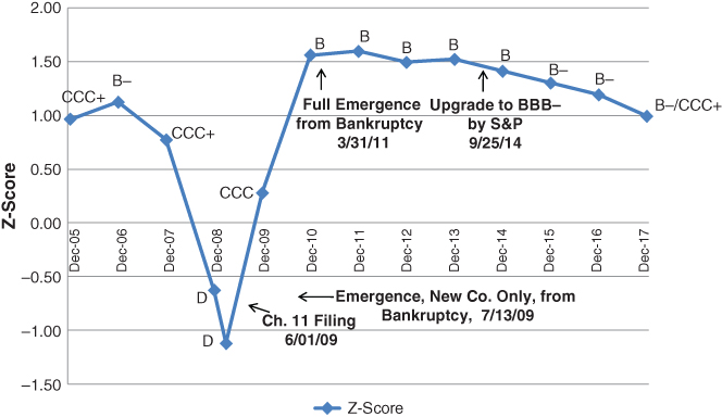
FIGURE 10.18 Z‐Score Model Applied to GM (Consolidated Data): Bond Rating Equivalents and Scores, 2005–2017
Note that GM's Z‐Score was in the CCC BRE, highly risky zone, for several years before the crisis in 2008, even when it was still rated investment‐grade by all of the rating agencies, for example, in 2005, see Figure 10.17. In addition, at the time of my testimony in December 2008, GM's score was –0.63, deep into the “D” BRE zone. Hence, I strongly suggested “Chapter 11” filing and that GM should petition the Bankruptcy Court for a $50 billion D.I.P. loan – most likely from the Federal Government since none of the major banks at that time were in sufficient financial shape to offer that size loan. The House of Representatives, and particularly its Finance Committee members, voted to continue the bailout, despite my arguments. The US Senate, however, voted not to continue the bailout, but President W. Bush, before leaving office, by Executive Order, provided the bailout to give GM and Chrysler more time to restructure. It was now “Obama's problem.” GM's Z‐score continued to crater in the early months of 2009 and despite management changes and the bailout, finally filed for bankruptcy under Chapter 11 on June 1, 2009. To assist the reorganization, Congress and the Bankruptcy Court provided a $50 billion DIP loan – that exact amount I suggested six months earlier!
In a remarkably short period, just 43 days, GM emerged from bankruptcy and was on its way toward once again being a going concern. Figure 10.17 shows the firm's improvement from deep into the D BRE to a B‐rating BRE in about 12–18 months. The DIP loan was first exchanged for new equity and that equity was subsequently sold in the open market, whereby not only did the government not lose any of its “investment,” it actually made a profit! GM today is a solid, thriving global auto competitor with, again, an investment‐grade rating (BBB) achieved in 2014. Note that the Z‐Score model, however, placed GM at the end of 2014 in the single‐B BRE, not investment‐grade; this low BRE continued through the end of 2018. So, while GM has indeed improved considerably since its bankruptcy, it still looked as noninvestment grade.
Comparative Risk Profile over Time
Students of history often ask the question of comparing a current situation with that of some past period(s). This query is particularly relevant in financial markets when the benchmark period in the past is related to some financial crisis and whether we can learn from the environment that existed then. Such is the case of the financial crisis of 2008/2009 and whether credit conditions today are similar, or not, to conditions just prior to that crisis. One metric that we have found useful in comparing credit market conditions over time is our Z‐Score models. Was the average (or median) firm credit worthiness better, worse, or about the same in, say 2016, compared to 2007? One might have some priors based on related macro or micro observations, such as cash on the balance sheet, interest rates or GDP growth. A more holistic, objective measure, in my opinion, is one, that is based on default probabilities that consider multiple attributes, such as the Z‐Score of a relevant sample of firms in the two periods.
Figure 10.19 shows the average and median Z and Z″ Scores for a large sample of high‐yield bond issuers in 2007 and 2016, with some intermediate years between the two periods. Observing these comparisons, we find extremely helpful in clarifying certain conclusions based on the qualitative or quantitative opinions of some experts. We find that the average Z‐Score was 1.95 (B+ BRE) in 2007 and 1.97 (also B+ BRE) in 2016 (3Q) and the median score was actually higher in 2007 (1.84) versus 1.70 in 2016. The average and median Z″‐Scores, a measure probably more appropriate given that the high‐yield firms in both periods came from many different industrial sector (see our discussion earlier about Z vs. Z″), were both higher in 2007 compared to 2016. Tests of the difference of means between 2007 and 2016 were found not to be significantly different, so our conclusion is that the average credit profile of risky‐debt issuing firms was about the same in 2007 versus 2016. I leave it up to the reader to determine if this was good or bad news for default estimates in 2017 and beyond.
* Bond rating equivalent.
FIGURE 10.19 Comparing Financial Strength of High‐Yield Bond Issuers in 2007 and 2012/2014/3Q 2016
Source: Authors' calculations, data from Altman and Hotchkiss (2006), and S&P Capital IQ/Compustat.
Predicting Defaults in Specific Sectors
Over the years, default cycles usually produce particular carnage in one or more industrial sectors and, if persistent for several years, these sectors draw particular attention to researchers and practitioners. Hence, for example, railroads (Altman 1973), the textile industry model (Altman et al. 1974), U.S. airlines (Altman and Gritta 1984), broker‐dealers (Altman 1976), and most recently, the energy and mining sectors in the United States, motivated specific analysis and tests.
A recent empirical test (Altman & Kuehne, 2017) of the Z‐Score models analyzed its accuracy in the energy and mining sectors. Rather than build a model based on energy‐firm data only, we decided to assess both the Z‐ and Z″‐Score models on a sample of bankruptcies in 2015, 2016 and 2017, a period when energy related firms accounted for more than half of the total defaults in those years. Figure 10.20 shows the results of just the bankruptcies, that is, Type I accuracy, for two periods prior to the filing of the 31 firms with data available for a Z‐Score test and even more firms (54) for the Z″‐Score test. Our results were quite impressive, especially for the Z‐Score model, which we built, as noted earlier, based only on manufacturing firm data. Indeed, 84% of the energy and mining companies had Z‐Scores in the D rating (Defaulted BRE), based on data from one or two quarters prior to the filing, and the remaining five firms in the sample had a CCC or B– BRE. For data from 5 or 6 quarters prior CCC; that is, only 2 out of 31 had a B rating BRE. While the results for the Z″‐Score model were not as accurate, 75% had a D BRE and the remaining firms had at least a B rating BRE, based on data from the last quarter prior to filing for bankruptcy, the results were still impressive and quite accurate.8

*One or two quarters before filing.
**Five or six quarters before filing.
FIGURE 10.20 Applying the Z‐Score Models to Recent Energy and Mining Company Bankruptcies, 2015–September 15, 2017
Source: S&P Capital IQ.
So, it appears that our original Z‐ and Z″‐Score models retain their high accuracy level for distress prediction, even for some industries not included in our original tests. We are not able to generalize, however, as to all nonmanufacturers, especially service firms.
Sovereign Default Risk
An intriguing application of the Z‐Score model is to use it to assess the default risk of sovereign nations' debt. We (Altman and Rijken 2011) were inspired by the World Bank study (Pomerleano 1998, 1999), which analyzed the causes of the financial crisis in Southeast and East Asia in 1997–1998 and found that the original Z‐Score model clearly demonstrated that the most vulnerable country to private sector defaults prior to the crisis was South Korea. Indeed, Korea had the lowest average Z‐Score for listed firms of all Asian countries, but was rated high investment‐grade by all of the rating agencies in December 1996. Yet, it needed to be bailed out by the IMF shortly thereafter! This illustration inspired us, more than a decade later, to analyze sovereign default risk in a unique way.
The aggregation of Z‐Scores, or in the case of Altman and Rijken's (2011) use of a more up‐to‐date version called Z‐MetricsT, proved to be exceptionally accurate in predicting the European countries with the most serious financial problems in the post‐2008 crisis. Their “Bottom‐Up” approach added a new microeconomic element to the arsenal of predictive measures for sovereign risk assessment, never before studied (See Chapter 13 herein for a detailed discussion).
Managing a Financial Turnaround
One of the most interesting and important applications of the Z‐Score model, from an internal and active, rather than passive standpoint of the distressed firm, is to apply the model as a guide to a successful turnaround of the firm. I suggested this application and wrote up a case study on the GTI Corporation, Altman and LaFleur (1981), also found in Altman and Hotchkiss (2006) and in Chapter 12 of this volume. The idea is a simple one; if a model is effective in predicting bankruptcy, why can't it be helpful to the management of the distressed firm in identifying the strategies and their impact on performance metrics. In the case of the GTI Corp., the new CEO, James LaFleur, strategically simulated the impact of his management changes on the resulting Z‐Scores, and only made those changes that resulted in an improved Z‐Score. His strategy did result in a remarkably successful turnaround. Here again was an application of the Z‐Score model that I (Altman) had never considered until a practitioner suggested its use.
CONCLUSION
The chapter has assessed the statistical and fundamental characteristics of Altman's 1968 Z‐Score model over the 50 years since the model's introduction. In addition, we have listed a large number of proposed and experienced applications of the original Z‐model and several subsequent ones, with a more detailed discussion of the specifics and importance of several of these applications. The 50‐year old model has demonstrated an impressive resilience over the years and, notwithstanding the massive growth in the size and complexity of global debt markets and corporate balance sheets, has shown not only longevity as an accurate predictor of corporate distress, but also that it has been successfully modified for a number of applications beyond its original focus. The list, shown in Figure 10.17, is almost assuredly incomplete, especially in view of the large number of scholarly works that have cited the Z‐Score models for a wide range of empirical research investigations. While we are surprised at the longevity of the Z‐Score models' usefulness, we now cannot help but wonder what some analysts might conclude in the year 2068 about its 100‐year track‐record.