Chapter Ten
Games of Pure Skill and Competitive Computers
Definitions
We define games of pure skill to be devoid of probabilistic elements. Such games are not often associated with monetary wagers, although formal admonishments against profiting from a skill are not proclaimed in most cultures. From a rational standpoint, it might be expected that a person should be far more willing to express financial confidence in his skills than on the mindless meanderings of chance. Experience, however, has strongly supported the reverse proposition.
The more challenging games of skill, some of which have resisted solution for centuries, exhibit either high space complexity (the number of positions in the search space) or high decision complexity (the difficulty encountered in reaching optimal decisions) or both. Generally, such games may be “solved” on three levels:
1. Ultra-weak. The game-theoretic value for the initial position has been determined. It might be proved, for example, that the first person to move will win (or lose or draw). Such a proof, sui generis, lacks practical value.
2. Weak. An algorithm exists that, from the opening position only, secures a win for one player or a draw for either against any opposing strategy.
3. Strong. An algorithm is known that can produce perfect play from any position against any opposing strategy (assuming not-unreasonable computing resources) and may penalize inferior opposing strategies.
Many of the games that have succumbed, at one of these levels, to the prowess of computer programs still retain an attraction, at least to the layman—particularly with strong solutions that involve complex strategies beyond the players’ memories or with weak solutions on large fields of play. The (weak) solution of Checkers, for example, has not intruded on the average person’s practice or understanding of the game.
Tic-Tac-Toe
Possibly the oldest and simplest of the games of pure skill is Tic-Tac-Toe (the name itself apparently derives from an old English nursery rhyme). With variations in spelling and pronunciation, its recorded history extends back to about 3500 B.C.—according to tomb paintings from Egyptian pyramids of that era.
Two players alternately place a personal mark (traditionally Xs and Os for the first and second players, respectively) in an empty cell of a matrix. Winner of the game is that player who configures his marks along an unbroken, complete line horizontally, vertically, or diagonally. In the event that neither player achieves such a line, the game is drawn (known colloquially as a “cat’s game”).
The generalized form of Tic-Tac-Toe entails a k × l matrix with each player striving for an n-in-a-row formation. Further generalizations expand the game to three or more dimensions and/or non-planar playing surfaces such as a cylinder, a torus, or a Möbius strip.
A 3 × 3 matrix with n = 3 constitutes the common form of Tic-Tac-Toe (Figure 10-1), with A designated as the first player, B the second. There are 138 unique games with this format, allowing for symmetries and winning positions that end the game before all nine cells are marked; the matrix itself has 8-fold symmetry. Of these, 91 are wins for X, 44 for O, while 3 are drawn. (Without symmetries, there are 255,168 possible games, 131,184 wins for X, 77,904 for O, 46,080 draws.) With rational play on the part of both players, no conclusion other than a draw will be reached.1 The opening move must be one of three: center (cell 5), corner (cells 1, 3, 7 or 9), or side (cells 2, 4, 6, or 8). Correct response to a center opening is placement of a mark in a corner cell (responding in a side cell leads to a loss). Correct response to a corner opening is occupying the center. To a side opening, the correct response is the center, adjoining corner, or far side. Additional counter-responses to a total of nine moves are readily obtained from only casual study.

Figure 10-1 The Tic-Tac-Toe matrix.
A simple but fundamental proof, known as the strategy-stealing argument, demonstrates that traditional Tic-Tac-Toe constitutes a draw or win for A. Postulate a winning strategy for B. A can then select any first move at random and thereafter follow B’s presumed winning strategy. Since the cell marked cannot be a detriment, we have a logical contradiction; ergo a winning strategy for the second player does not exist.
The basic Tic-Tac-Toe game can be extended to matrices larger than 3 × 3 (Ref. Ma). For n = 3, A wins on all matrices k ≥ 3, l > 3. For n = 4, the game is a draw on a 5 × 5 matrix but a win for A on all matrices k ≥ 5, l > 5 (including the infinite board). The n = 5 game, when played on matrices 15 × 15 or greater, offers a forced win for A (Ref. Allis, van der Meulen, and van den Herik) and is known as Go-Moku (Japanese: gomoku narabe, line up five) when adapted to the intersections on a (19 × 19) Go board (Ref. Allis, van den Herik, and Huntjens). With n = 6, the game is a draw on a 6 × 6 matrix and unsolved on all larger matrices. Games with n > 6 on larger (and infinite) matrices are drawn under rational decision-making.
An efficient procedure for determining whether a particular Tic-Tac-Toe format leads to a draw is that of the Hales-Jewett pairing strategy (Ref. Hales and Jewett). Figure 10-2 illustrates this strategy for n = 5 on a 5 × 5 matrix.

Figure 10-2 A Hales-Jewett pairing.
Each square is assigned a direction: north-south, east-west, northeast-southwest, or northwest-southeast. Then, for every square occupied by A, B occupies the similarly marked square in the direction indicated by the slash. Accordingly, B will have occupied at least one square in every possible line of five squares—and will thereby have forced a draw. (Further, B can concede to A the center square and the first move and still draw the game.)
The Hales-Jewett pairing strategy is especially useful for higher values of n on large matrices.
Variants of Tic-Tac-Toe extend back more than two millennia. Following are some of the more noteworthy.
Misère Tic-Tac-Toe
Whoever first places his marks collinearly loses. For n = 3 on a 3 × 3 matrix, the “X” player can ensure a draw by occupying the center square and thereafter countering the “O” moves by reflecting them through the center. With an even value for k or l, B, using this strategy, has at least a draw for any n.
Wild Tic-Tac-Toe
Players may use either an X or O for each move. This variant offers limited appeal since A has a forced win by placing a mark in the center cell.
Wild Misère Tic-Tac-Toe
The first player to complete three-in-a-row (with either mark) loses. The second player can force a draw by marking a cell directly opposite his opponent’s moves, choosing X against O and O against X.2
Kit-Kat-Oat
Each participant plays his opponent’s mark. The disadvantage lies with A; he can achieve a draw, however, by placing his opponent’s mark in the center cell as his first move and thereafter playing symmetrically about the center to his opponent’s previous move.
Kriegspiel Tic-Tac-Toe
Each player is accorded a personal 3 × 3 matrix, which he marks privately (unseen by his opponent). A referee observes the two matrices and ensures that corresponding cells are marked on only one matrix by rejecting any moves to the contrary. Since A, as first player, possesses a pronounced advantage, it is reasonable to require that he be handicapped by losing a move upon receiving a rejection, while B is guaranteed a legal move at each turn. Imposition of this handicap reduces, but does not eliminate A’s advantage. Played on 4 × 4 matrices, the game still offers a slight edge to A. A remaining unsolved problem is to ascertain the size of the matrix whereby, under the handicap rule, Kriegspiel Tic-Tac-Toe becomes a fair game.
Tandem Tic-Tac-Toe
Each player possesses his personal 3 × 3 cellular matrix, which he labels with the nine integers 1, 2, …, 9, each cell being marked with a distinct integer. The marking process occurs one cell at a time—first as a concealed move, which is then exposed simultaneously with his opponent’s move. With the information obtained, a second cell of each array is marked secretly, then revealed, and so forth, until all nine cells of both matrices are numbered. For the second phase of the game, A places an X in a cell in his matrix and in the same-numbered cell in his opponent’s matrix. B then selects two similarly matching cells for his two Os, and so forth. If a win (three collinear personal symbols) is achieved in one matrix, the game continues in the other matrix. Clearly, both players strive for two wins or a single win and a tie. B’s evident strategy is to avoid matching of the center and corner cells between the two matrices.
Rook-Rak-Row
Each player, in turn, may place one, two, or three marks in a given row or column of the 3 × 3 matrix (if two cells are marked, they need not be adjacent). Whichever player marks the last cell wins the game. B can always force a win. If A places a single X, B counters with two Os that form a connected right angle. If A marks two or three cells, B marks three or two cells, respectively, to form a “T,” an “L,” or a cross composed of five cells.
Cylindrical Tic-Tac-Toe
The top and bottom of a k × l matrix are connected. For n = 3 on a 3 × 3 matrix, two additional collinear configurations are possible: 4-8-3 and 6-8-1.
Toroidal Tic-Tac-Toe
Both top and bottom and left and right sides of the playing matrix are connected (thus forming a torus). All opening moves are equivalent. With matrices of 3 × 3 or 2 × l, l ≥ 3, A can force a win for the n = 3 game. For n = 4, A wins on a 2 × l matrix for l ≥ 7, while the n = 5 game is a draw on any 2 × l matrix.
Möbius Strip Tic-Tac-Toe
Here, cells 1, 2, 3 are connected to cells 9, 8, 7.
Algebraic Tic-Tac-Toe
A first selects a value for any one of the nine coefficients in the system of simultaneous equations
 (10-1)

 (10-2)
Then B assigns a value to one of the remaining eight coefficients, and so forth. A wins the game if the completed system has a non-zero solution.
Winning strategy for A: Select any value for coefficient b2 and thereafter play symmetrically to B—so that after all nine coefficients have been assigned values we have

Thence Eqs. 10-1 and 10-2 are equivalent. Since the system of simultaneous equations is homogeneous, it is consistent and admits of infinitely many solutions—including a non-(0, 0, 0) solution. Thus the game is a win for A.
Numerical Tic-Tac-Toe
A and B alternately select an integer from the set 1, 2, …, 9, placing it in one cell of the 3 × 3 matrix (Ref. Markowsky). Objective: to achieve a line of three numbers that sums to 15. This game is isomorphic to standard Tic-Tac-Toe—as per the correspondence shown in the magic square of Figure 10-3. A is afforded an easy win—on his second move if he begins with the center cell 5, on his third move if he begins with a corner or side cell.

Figure 10-3 Tic-Tac-Toe magic square.
Considerably greater complexity ensues if the set of integers is divided between A (permitted to place only the odd integers) and B (permitted to place only the even integers).
Three-Dimensional Tic-Tac-Toe
Surprisingly, the 3 × 3 × 3 game with n = 3 proves uninteresting since A has a simple forced win by marking the center cell; failure to follow this strategy allows B to do so and thereby usurp the win. The game cannot be drawn since it is impossible to select 14 of the 27 cells without some three being collinear, either orthogonally or diagonally.
Draws are possible with n = 4 played on a 4 × 4 × 4 lattice.3 Here the two players alternately place their counters in one of the 64 cubicles. Objective: to achieve a line of (four) connected personal counters either in a row, a column, a pillar, a face diagonal, or a space diagonal.
This game was weakly solved by Oren Patashnik (in 1980) and subsequently (in 1994) strongly solved by Victor Allis using proof-number search, confirming that the first player can effect a win.
Three-Dimensional Misère Tic-Tac-Toe
The n = 3 game offers a win for A—by applying the same strategy as in planar Misère Tic-Tac-Toe: first marking the center cell and thereafter playing symmetrically opposite his opponent. (Since drawn games are impossible, this strategy forces B ultimately to mark a collinear pattern.)
The n = 4 misère game, similar to standard three-dimensional 4 × 4 × 4 Tic-Tac-Toe, likewise admits of drawn positions.
Higher-Dimensional Tic-Tac-Toe
Since two-dimensional Tic-Tac-Toe exists logically for two players, we might infer that the three- and four-dimensional versions can be constructed for three and four players, respectively. In d dimensions, a player can achieve a configuration with d potential wins so that the d − 1 succeeding players cannot block all the means to a win.
Two-person, d-dimensional Tic-Tac-Toe offers some mathematical facets. Played in an n×n× … ×n (d times) hypercube, the first player to complete any line-up of n marks wins the game—and there are [(n + 2)d − nd]/2 such lines (which for n = 3 and d = 2—the standard planar game—is equal to 8; for the n = 4, d = 3 game, there are 76 winning lines). B can force a draw (with the appropriate pairing strategy) if n ≥ 3d − 1 (n odd) or n ≥ 2d+1 − 2 (n even). However, for each n there exists a dn such that for d ≥ dn, A can win (Ref. Ma).
Construction of games in d ≥ 4 dimensions presents difficulties in our three-dimensional world. It has been proved that a draw exists for n≥cd log d, where c is a constant (Ref. Moser).
Misère Higher-Dimensional Tic-Tac-Toe
S.W. Golomb has shown that A can achieve at least a draw in a d-dimensional hypercube of side n whenever n ≥ 3 is odd (Ref. Golomb and Hales). A marks the center cell initially and thereafter plays diametrically opposite each opponent move. (Thus A will never complete a continuous line-up through the center cell, and any other possible line can only be a mirror image of such a line already completed by B.)
Random-Turn Tic-Tac-Toe
A coin toss determines which player is to move. The probability that A or B wins when both play optimally is precisely the probability that A or B wins when both play randomly (Chapter 9, Random Tic-Tac-Toe).
Moving-Counter Tic-Tac-Toe
This form, popular in ancient China, Greece, and Rome, comprises two players, each with three personal counters. A and B alternately place a counter in a vacant cell of the 3 × 3 matrix until all six counters have been played. If neither has succeeded in achieving a collinear arrangement of his three counters, the game proceeds with each player moving a counter at his turn to any empty cell orthogonally adjacent. A has a forced win by occupying the center cell as his opening move.
Other versions, which result in a draw from rational play, permit diagonal moves or moves to any vacant cell.
Tic-Tac-Toe with moving counters has also been adapted to 4 ×4 and 5 ×5 matrices. In the latter example, invented by John Scarne (Ref.) and called Teeko (Tic-tac-toe chEss chEcKers bingO), two players alternately place four personal counters on the board followed by alternating one-unit moves in any direction. Objective: to maneuver the four personal counters into a configuration either collinear or in a square formation on four adjacent cells (the number of winning positions is 44). Teeko was completely solved by Guy Steele (Ref.) in 1998 and proved to be a draw.
Multidimensional moving-counter games—“hyper-Teeko”—remain largely unexplored.
Finally, quantum Tic-Tac-Toe (Ref. Goff) allows players to place a quantum superposition of numbers (“spooky” marks) in different matrix cells. When a measurement occurs, one spooky mark becomes real, while the other disappears.
Computers programmed to play Tic-Tac-Toe have been commonplace for close to seven decades. A straightforward procedure consists of classifying the nine cells in order of decreasing strategic desirability and then investigating those cells successively until it encounters an empty one, which it then occupies. This process can be implemented by relays alone.
A simple device that converges to an optimal Tic-Tac-Toe strategy through a learning process is MENACE (Matchbox Educable Noughts And Crosses Engine), a “computer” constructed by Donald Michie (Ref.) from about 300 matchboxes and a number of variously colored small glass beads (beads are added to or deleted from different matchboxes as the machine wins or loses against different lines of play, thus weighting the preferred lines). Following an “experience” session of 150 plays, MENACE is capable of coping (i.e., drawing) with an adversary’s optimal play.
Another simple mechanism is the Tinkertoy computer, constructed by MIT students in the 1980s, using, as its name implies, Tinker Toys.
More sophisticated is the Maya-II, developed at Columbia University and the University of New Mexico, which adapts a molecular array of YES and AND logic gates to calculate its moves. DNA strands substitute for silicon-based circuitry. Maya-II brazenly always plays first, usurps the center cell, and demands up to 30 minutes for each move.
Nim and Its Variations
A paradigmatic two-person game of pure skill, Nim is dubiously reputed to be of Chinese origin—possibly because it reflects the simplicity in structure combined with subtle strategic moves (at least to the mathematically unanointed) ascribed to Oriental games or possibly because it was known as Fan-Tan (although unrelated either to the mod 4 Chinese counter game or the elimination card game) among American college students toward the end of the 19th century.
The word Nim (presumably from niman, an archaic Anglo-Saxon verb meaning to take away or steal) was appended by Charles Leonard Bouton (Ref.), a Harvard mathematics professor, who published the first analysis of the game in 1901. In the simplest and most conventional form of Nim, an arbitrary number of chips is apportioned into an arbitrary number of piles, with any admissible distribution. Each player, in his turn, removes any number of chips one or greater from any pile, but only from one pile. That player who removes the final chip wins the game.
In the terminology of Professor Bouton, each configuration of the piles is designated as either “safe” or “unsafe.” Let the number of chips in each pile be represented in binary notation; then a particular configuration is uniquely safe if the mod 2 addition of these binary representations (each column being added independently) is zero; this form of addition, known as the digital sum, is designated by the symbol  . For example, three piles consisting of 8, 7, and 15 chips are represented as follows:
| 8 | = | 1000 |
| 7 | = | 111 |
| 15 | = | 1111 |
| Digital sum | = | 0000 |
and constitute a safe combination. Similarly, the digital sum of 4 and 7 and 2 is 100  111
111  10 = 1; three piles of four, seven, and two chips thus define an unsafe configuration.
It is easily demonstrated that if the first player removes a number of chips from one pile so that a safe combination remains, then the second player cannot do likewise. He can change only one pile and he must change one. Since, when the numbers in all but one of the piles are given, the final pile is uniquely determined (for the digital sum of the numbers to be zero), and since the first player governs the number in that pile (i.e., the pile from which the second player draws), the second player cannot leave that number. It also follows, with the same reasoning, that if the first player leaves a safe combination, and the second player diminishes one of the piles, the first player can always diminish some pile and thereby regain a safe combination. Clearly, if the initial configuration is safe the second player wins the game by returning the pattern to a safe one at each move. Otherwise, the first player wins.
Illustratively, beginning with three piles of four, five, and six chips, the first player performs a parity check on the columns:
| 4 | = | 100 |
| 5 | = | 101 |
| 6 | = | 110 |
| Digital sum | = | 111 |
Bouton notes that removing one chip from the pile of four, or three chips from the pile of five, or five chips from the pile of six produces even parity (a zero digital sum, a safe position) and leads to a winning conclusion. Observe that from an unsafe position, the move to a safe one is not necessarily unique.
A modified version of Nim is conducted under the rule that the player removing the last chip loses. The basic strategy remains unaltered, except that the configuration 1, 1, 0, 0, …, 0 is unsafe and 1, 0, 0, …, 0 is safe.
If the number of counters initially in each pile is selected at random, allowing a maximum of 2m−1 chips per pile (m being any integer), the possible number of different configurations N with k piles is described by

Frequently Nim is played with three piles, whence
The number of safe combinations Ns in this case is

Thus, the probability Ps of creating a safe combination initially is given by
which is the probability that the second player wins the game, assuming that he conforms to the correct strategy.
Moore’s Nim
A generalization of Nim proposed by E.H. Moore (Ref.) allows the players to remove any number of chips (one or greater) from any number of piles (one or greater) not exceeding k. Evidently, if the first player leaves fewer than k + 1 piles following his move, the second player wins by removing all the remaining chips. Such a configuration is an unsafe combination in generalized Nim. Since the basic theorems regarding safe and unsafe patterns are still valid, a player can continue with the normal strategy, mod (k + 1), until the number of piles is diminished to less than k + 1, whence he wins the game.
To derive the general formula for safe combinations, consider n piles containing, respectively, c1, c2, …, cn chips. In the binary scale of notation,4 each number ci is represented as ci = ci0 + ci1 21 + ci2 22 +…+ cij2j. The integers cij are either 0 or 1 and are uniquely determinable. The combination is safe if and only if

that is, if and only if for every place j, the sum of the n digits cij is exactly divisible by k + 1.
Moore’s generalization is referred to as Nimk. Bouton’s game thus becomes Nim1 and provides a specific example wherein the column addition of the chips in each pile is performed mod 2.
Matrix Nim
Another generalization, termed Matrix Nim and designated by Nimk (nomenclature applied by John C. Holladay (Ref.) to distinguish the game from Moore’s version), consists of arranging the k piles of chips into an m × n rectangular array. For a move in this game, the player removes any number of chips (one or greater) from any nonempty set of piles, providing they are in the same row or in the same column, with the proviso that at least one column remains untouched. The game concludes when all the piles are reduced to zero, the player taking the final chip being the winner. Nimk with k = 1 becomes, as with Moore’s generalization, the ordinary form of Nim.
A safe position in Nimk occurs if the sum of the chips in any column is equal to the sum of the chips in any other column and if the set of piles defined by selecting the smallest pile from each row constitutes a safe position in conventional Nim.
Shannon’s Nim
In a Nim variation proposed by Shannon Claude (Ref. 1955), only a prime number of chips may be removed from the pile. Since this game differs from Nim1 only for those instances of four or more chips in a pile, a safe combination is defined when the last two digits of the binary representations of the number of chips in each pile sum to 0 mod 2. For example, a three-pile game of Nim1 with 32, 19, and 15 chips provides a safe configuration in Shannon’s version, although not in the conventional game. This situation is illustrated as follows:
| 15 | = | 1111 |
| 19 | = | 10011 |
| 32 | = | 100000 |
| Digital sum | = | 111100 |
It should be noted that the basic theorems of safe and unsafe combinations do not hold for prime-number Nim1.
Wythoff’s Nim—Tsyan/Shi/DziI
Obviously, we can impose arbitrary restrictions to create other variants of Nim. For example, a limit can be imposed on the number of chips removed or that number can be limited to multiples (or some other relationship) of another number. A cleverer version, credited to W.A. Wythoff (Ref.) restricts the game to two piles, each with an arbitrary number of chips. A player may remove chips from either or both piles, but if from both, the same number of chips must be taken from each. The safe combinations are the Fibonacci pairs: (1, 2), (3, 5), (4, 7), (6, 10), (8, 13), (9, 15), (11, 18), (12, 20), … . The rth safe pair is ([rτ], [rτ2]), where τ = (1 + )/2, and [x] is defined as the greatest integer not exceeding x. Note that every integer in the number scale appears once and only once. Although evidently unknown to Wythoff, the Chinese had long been playing the identical game under the name of Tsyan/shi/dzi (picking stones).
Unbalanced Wythoff
One extension of Wythoff’s game (Ref. Fraenkel, 1998) defines each player’s moves as either (1) taking any (positive) number of counters from either pile, or (2) removing r counters from one pile and r ≤ s from the other. This choice is constrained by the condition 0 ≤ s—r < r + 2, r > 0. That player who reduces both piles to zero wins.
The recursion expressions for this game (for all values of n ≥ 0) are


which generate the safe positions shown in Table 10-1. The player who leaves any of these pairs for his opponent ultimately wins the game.
Table 10-1. Safe Positions for Unbalanced Wythoff
Four-Pile Wythoff
A further extension of Wythoff’s game—devised by Fraenkel and Zusman (Ref.)—is played with k ≥ 3 piles of counters. Each player at his turn removes (1) any number of counters (possibly all) from up to k − 1 piles, or (2) the same number of counters from each of the k piles. That player who removes the last counter wins.
For k = 4, the first few safe positions are listed in Table 10-2. The player who reduces the four piles to any of these configurations ultimately wins the game.
Table 10-2. Safe Positions for Four-Pile Wythoff

The Raleigh Game (After Sir Walter Raleigh for no discernible reason)
In this yet further extension of Wythoff’s game proposed by Aviezri Fraenkel (Ref. 2006), the format encompasses three piles of chips, denoted by (n1, n2, n3), with the following take-away rules:
1. Any number of chips may be taken from either one or two piles.
2. From a position where two piles have an equal number of chips, a player can move to (0, 0, 0).
3. For the case where 0 < n1 < n2 < n3, a player can remove the same number of chips m from piles n2 and n3 and an arbitrary number from pile n1—with the exception that, if n2 − m is the smallest component in the new position, then m ≠ 3.
The safe positions for Raleigh, (An, Bn, Cn), are generated from the recursive expressions


and are tabulated in Table 10-3. The player who configures the three piles into one of these positions can force a win.
Table 10-3. Safe Positions for the Raleigh Game

Nimesis (Ref. Cesare and Ibstedt)
A, accorded the first move, divides a pile of N counters into two or more equal-sized piles and then removes a single pile to his personal crib. B, for his move, reassembles the remaining counters into a single pile and then performs the same operation. A and B continue to alternate turns until a single counter remains. That player whose crib holds the greater number of counters wins the game.
To compensate for A’s moving first, B selects the value of N. With N restricted to numbers under 100, B’s optimal strategy is to select that N for which both N and

are prime for all values of i from 0 to  where [x] denotes the largest integer within x. Only N = 47 satisfies these conditions.
For the first step of the game, A must, perforce, divide the 47 counters into 47 piles of 1 counter each. B will then divide the remaining 46 counters into two piles of 23 counters. Over the five steps defining the complete game, A will accrue 5 counters, and B will garner 23 + 11 + 5 + 2 + 1 = 42 counters. Thus B has a winning fraction of 42/47 = 0.894.
With N allowed a value up to 100,000, B selects N = 2879. Thence A’s counters total 1 + 1 + 1 + 1 + 1 + 1 + 22 + 1 + 1 + 1 = 31, while B’s counters add up to 1439 + 719 + 359 + 179 + 89 + 44 + 11 + 5 + 2 + 1 = 2848. Accordingly, B’s winning fraction is 2848/2879 = 0.989. As the allowable upper limit is raised, the winning fraction for B—already high—approaches yet closer to 1.
Tac Tix
Another ingenious Nim variation, one that opens up an entire new class, was proposed by Piet Hein5 under the name Tac Tix (known as Bulo in Denmark). The game, which follows logically from Matrix Nim, deploys its chips in an n × m array. Two players alternately remove any number of chips either from any row or from any column, with the sole proviso that all chips taken on a given move be adjoining.
Tac Tix must be played under the rule that the losing player is the one removing the final chip. Otherwise, there exists a simple strategy that renders the game trivial: the second player wins by playing symmetrically to the first player unless the matrix has an odd number of chips in each row and column, in which case the first player wins by removing the center chip on his first move and thereafter playing symmetrically to his opponent. No strategy is known for the general form of Tac Tix. In the 3 × 3 game the first player can always win with proper play (his first move should take the center or corner chip or the entire central row or column). As a practical contest between sophisticated game theorists, the 6 × 6 board is recommended.
Chomp
A Nim-type game invented by David Gale (Ref. 1974), Chomp (the name appended by Martin Gardner) postulates an M by N chocolate bar whose upper-left corner square (1, 1) is poisonous. Two players alternately select a square, which is eaten along with all other squares below and to its right. The initial position consists of the whole bar (i, j), where 1 ≤ i ≤ M, and 1 ≤ j ≤ N. Thus the player who selects the square (io, jo) must perforce eat all the remaining squares where both i ≥ io and j ≥ jo. He who eats the poisonous square loses.
The game is celebrated for Gales’s Chomp existence theorem—akin to the strategy-stealing argument of Tic-Tac-Toe. Consider that the first player eats square (M, N), the lower-right corner—leaving MN−1 squares. This act constitutes either a winning move or a losing move; if the latter, then the second player has a winning countermove. However, any position reachable from the new array with MN−1 squares is also reachable from the initial array with MN squares. Hence the first player could have moved there directly. There exists, ipso facto, a winning move for the first player.
Nim-Like Games
Numerous games have been proposed that, on cursory inspection, appear difficult to analyze but succumb quickly when their structures are recognized as Nim-like in form. Such games are referred to as NimIn (for Nim Incognito).
Perhaps the simplest type of NimIn involves “coins on a strip.” Consider the format depicted in Figure 10-4. A and B alternate in moving any coin any number of squares leftward. Only a single coin may occupy any one square, and no coin may jump over another. The game ends when all the coins are lined up at the left end of the strip; the player who achieves this configuration wins.

Figure 10-4 A simple NimIn game.
The key in this instance is the recognition that the lengths of the gaps between coins—beginning with the rightmost—are simply the sizes of the equivalent Nim piles. Then the initial nim-sums in Figure 10-4 are
| 2 | = | 10 |
| 0 | = | 0 |
| 3 | = | 11 |
| Digital sum | = | 01 |
which constitute an unsafe position. A winning move reduces the gap of three squares to two squares, leaving
| 2 | = | 10 |
| 0 | = | 0 |
| 2 | = | 10 |
| Digital sum | = | 00 |
a safe position. (Note that an increase in a gap length is possible by moving the left coin of a pair. However, the winning strategy remains unaffected.)
A somewhat more interesting variant is Stepine’s game: played with n coins and a gold piece arrayed at intervals along a line whose left-hand side terminates in a moneybag—illustrated in Figure 10-5 for six coins and the gold piece. A move (by each of two players in successive turns) consists of shifting any coin or the gold piece any number of empty spaces leftward. When a coin is moved to the leftmost space, it falls into the moneybag. That player who deposits the gold piece in the moneybag takes it home.

Figure 10-5 Stepine’s game.
Again, the resolution of Stepine’s game lies in recognizing its Nim-like structure. Accordingly, the coins (and gold piece) should be considered pairwise beginning at the right. The number of pairs corresponds to the number of piles, and the number of spaces within each pair to the number of chips in that pile in the Nim1 equivalency. If a coin is left unpaired, the winning strategy includes the money-bag space if the gold piece forms the left side of a pair and excludes the money-bag space if it forms the right side of a pair (if the gold piece is leftmost, it can be moved directly into the money bag). In the example of Figure 10-5, we compute the digital sum of 3, 4, 1, and 7—which is nonzero. A winning move consists of reducing the 3, 1, or 7 interval by one.
Superficially more complicated is Northcott’s Nim. Here, the playing field is an n × m checkerboard. Each row of the board holds a white piece and a black piece. For his turn, White may move any one of his pieces along its row, in either direction, as far as the empty squares allow. Black then moves any one of his pieces under the same rules. The game proceeds in this manner until one player cannot move—and thereby loses.
Northcott’s Nim is equivalent to Nim1 with a pile of chips for each row. The number of chips in a particular pile is equivalent to the number of squares between the black and white pieces in the corresponding row. (Each player’s prerogative to increase the space between black and white pieces does not alter the character of the game or its ultimate convergence.)
Unsolved Nim variants
1. Nimk played under the restriction that chips may be removed only from a prime number of piles.
2. Wythoff’s Nim played with the option of removing simultaneously from the two piles an arbitrary ratio a:b of chips (rather than an equal number).
3. Wythoff’s Nim played with three or more piles, where the player is awarded the option of removing the same number of chips simultaneously from each pile.
4. Tac Tix played with upper and lower limits placed on the number of chips that may be removed at each move.
5. Tac Tix played with the option of removing the same number of chips in both directions from a row-column intersection.
Nim Computers
A Nim1-playing computer should logically be a relatively simple device because of the binary nature of the strategy. Nimatron, the first such computer, was patented in 1940 by Edward Condon (Ref.), former director of the National Bureau of Standards. Built by the Westinghouse Electric Corp, Nimatron was exhibited at the New York World’s Fair, where it played 100,000 games, winning about 90,000 (most of its defeats were administered by attendants demonstrating that possibility). At present, it reposes in the scientific collection of the Buhl planetarium in Pittsburgh. One year later, a vastly improved machine was designed by Raymond M. Redheffer (Ref.). Both the Redheffer and Condon computer programs were devised for play with four piles, each containing up to seven chips.
Subsequently, a Nim1-playing device named Nimrod was exhibited at the 1951 Festival of Britain and later at the Berlin Trade Fair. A different approach to Nim was expressed through a simple relay computer developed at the Research Institute of Mathematical Machines (Prague) in 1960. This machine, programmed with knowledge of the optimal strategy, is pitted against a mathematical neophyte. The designated objective is to achieve a victory while disclosing as little information as possible regarding the correct game algorithm. Hence the computer applies its knowledge sparingly as a function of its opponent’s analytic prowess.
Single-Pile Countdown Games
Although not linked by firm evidence, it is likely that Nim is related to a game described by Bachet de Mésiriac in the early 17th century. From a single pile comprising an arbitrary number of chips, each of two players alternately removes from one to a chips. The winner is that player who reduces the pile to zero. Thus, a safe position in Bachet’s game occurs when the number of chips in the pile totals 0, mod (1 + a).
Single-pile games6 can be formulated by specifying any restricted set of integers S = {n1, n2, …} that prescribes the number of chips that may be taken from the pile at each move. For each such set of integers, there exist positions (states) of the pile that are winning, losing, or tying for the player confronted with a move. Designating the winning and losing states by W(S) and L(S), respectively, we observe that

and

that is, the union of the winning and losing sets includes all nonnegative integers, while the intersection of these sets is empty, under the assumption that the set of tying positions T(S) = Ø—an assumption valid if and only if 0 is not a member of the subtractive set S and if 1 is a member of S. For greater harmony, it is advisable to include the number 1 in the subtractive set and to designate the winner as that player reducing the pile to zero.
As in the various Nim games, every member of S added to a member of L(S) results in a member of W(S). Thus, a losing or safe position is always attainable from a winning or unsafe position, but not from another safe position.
Two subtractive sets S1 and S2 are characterized as game isomorphic if they define games with identical losing states. For example, the set of all positive powers of two, S1 = {1, 2, 4, 8, …}, is game isomorphic to S2 = {1, 2} since

(no power of 2 is a multiple of 3), and the set of primes, S1 = {1, 2, 3, 5, 7, …}, is game isomorphic to S2 = {1, 2, 3}, since

(no prime is a multiple of 4). Thus, a single-pile countdown game where only a prime number of chips may be subtracted can be won by the first player to reduce the pile to a multiple of 4.
It can be demonstrated that game isomorphism is closed under union, but not under intersection. For example, consider the two subtractive sets S1 = {1, 4, 5} and S2 = {1, 3, 4, 7}. We compute L(S1) by the paradigm shown in Table 10-4. The sequence of L(S1) is determined by entering in the L(S1) column the lowest integer not previously represented; that integer is then added to 1, 4, and 5, respectively, and the sum entered in the corresponding column, etc. Evidently, L(S1) = {0, 2, mod 8}. By the same technique, we can also calculate L(S2) = {0, 2, mod 8} and show that  = {0, 2, mod 8}, whereas
  = {0, 2, mod 5}.
Table 10-4. Computation of Losing States L(S1)

To complete our understanding of the sets that exhibit game isomorphism, we introduce the states λ(S) as all the nonnegative first differences of L(S). We can prove that λ(S) cannot intersect S—that is,

and the converse statement that any number not in λ(S) can be adjoined into S. Illustratively, consider the set S = {1, 4}, which generates the set of losing positions L(S) = {0, 2, mod 5}. In this instance, the numbers 3, mod 5, are obtained by first differences of the other members of L(S), so that λ(S) = {0, 2, 3, mod 5}. All remaining numbers (1, mod 5 and 4, mod 5) can be adjoined to S:

Thus, any set S* is game isomorphic to S. For example, the game played with S={1, 4} is equivalent (in the sense of identical losing positions) to that played with S* = {1, 4, 9, 16}.
Given a particular subtractive set, it is not always possible to find another set with the property of game isomorphism. As one instance, consider the game whereby, from an initial pile of m chips, each player alternately subtracts a perfect-square number of chips, S = {1, 4, 9, 16, …}, with the usual objective of removing the final chip to score a win. It is not apparent that a simple formula exists that determines the safe positions L(S) for this game. However, as demonstrated by Golomb, the sequence of safe positions can be generated by an appropriately constructed shift register.
A binary shift register is a simple multistage device whereby, in a given configuration, each stage exhibits either a 1 or a 0. At prescribed intervals the output of each stage of the register assumes the value represented by the output of the previous stage over the previous interval. The outputs from one or more stages are operated on in some fashion and fed back into the first stage. For the single-pile countdown game with S = {1, 4, 9, 16, …}, the appropriate shift register is of semi-infinite length, since the perfect squares form an infinite series. The outputs of stages 1, 4, 9, 16, … are delivered to a NOR gate and thence returned to the first stage.
Figure 10-6 indicates the perfect-square shift register. Initially, the first stage is loaded with a 1 and the remaining stages with 0s. If at least one 1 enters the NOR gate, it feeds back a 0 to the first stage as the register shifts; otherwise, a 1 is fed back. The continuing output of the shift register designates the safe and unsafe positions, with 1 representing safe and 0 unsafe. Table 10-5 illustrates the shift-register performance. According to the output sequence, positions 2, 5, and 7 (of the first 8) are safe; that is, if a player reduces the pile of chips to 2, 5, or 7, he possesses a winning game, since his opponent can achieve only an unsafe position.
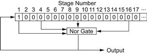
Figure 10-6 The perfect-square shift register.
Table 10-5. The Perfect-Square Shift Register Output

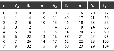
Allowing the perfect-square shift register to run for 1000 shifts produces 1s at the positions shown in Table 10-6. Thus, beginning with a pile of 1000 or less, the player who reduces the pile to any of the positions shown in this table can achieve a win.
Table 10-6. The Safe Positions for the Perfect-Square Game

There are 114 safe positions for a pile of 1000 chips, 578 safe positions for a pile of 10,000 chips, and 910 safe positions for a pile of 20,000 chips. Evidently, as m, the number of initial chips, increases, the percentage of safe positions decreases. The totality of safe positions is infinite, however, as m → ∞ (there exists no largest safe position).
A substantial number of engaging single-pile countdown games can be invented. As one example, we can regulate each player to subtract a perfect-cube number of chips. For this game, the semi-infinite shift register of Figure 10-6 is rearranged with the outputs of stages 1, 8, 27, 64, … fed to the NOR gate. The output of such a shift register indicates safe positions at 2, 4, 6, 9, 11, 13, 15, 18, 20, 22, 24, 34, 37, 39, 41, 43, 46, 48, 50, 52, 55, 57, 59, 62, 69, 71, 74, 76, 78, 80, 83, 85, 87, 90, 92, 94, 97, 99, … .
The shift register method can also be enlisted to solve more elementary countdown games. Consider Bachet’s game with a = 4—that is, S = {1, 2, 3, 4}. In this instance we construct a finite four-stage shift register (the number of stages required is specified by the largest member of S) with the outputs of all four stages connected to the NOR gate, as shown in Figure 10-7. Inserting a 1 into the first stage and 0s into the remaining stages and permitting the shift register to run results in the output sequence 00001000010000100…; the safe positions occur at 0, mod 5, as we would expect.

Figure 10-7 Shift register for Bachet’s game.
Several extensions of Bachet’s game are worthy of note. For one example, we might impose the additional constraint that each player must remove at least b chips (but no more than a > b) at each move. A win is awarded to that player reducing the pile to b − 1 or fewer chips. The safe positions here are 0, 1, 2, …, b − 1, mod (b + a). If different limits are assigned to each player, the possessor of the larger limit can secure the winning strategy.
Another offspring of Bachet’s game arises from the restriction that the same number of chips (of the set S = {1, 2, …, a}) cannot be subtracted twice in succession. If a is even, no change is effected by this rule: L(S) = {0, mod (a + 1)}. If a is odd, correct strategy is altered in certain critical positions; for example, with a = 5 and six chips remaining, the winning move consists of subtracting 3 chips, since the opponent cannot repeat the subtraction of 3. Specifically, for a = 5, L(S) = {0, 7, mod 13}. For any odd value of a except 1 and 3, L(S) = {0, a + 2, mod (2a + 3)}; for a = 3, L(S) = {0, mod 4}.
Slim Nim (Sulucrus)
A and B alternately remove counters from a single pile of N counters (N > 22). A has the option at each turn of removing 1, 3, or 6 counters; B at his turn may remove 2, 4, or 5. Objective: to remove the last counter(s). The game is a win for B regardless of which player moves first (Ref. Silverman).
If N is of the form 2, mod 5 or 4, mod 5, B, at his first turn, subtracts 2 or 4 chips, respectively, and thereafter counters a move by A (1, 3, or 6) with a move complementary to 0, mod 5—that is, 4, 2, or 4.
If N is of the form 3, mod 5, B subtracts 5 at his first turn and thereafter again moves to reduce the pile to 0, mod 5—removing 2, 5, 2 against 1, 3, 6, respectively.
Finally, if N is of the form 1, mod 5, B removes 5 chips and thereafter subtracts 5 against a move of 1 or 6. Against a reduction of 3 chips by A, B is left with 3, mod 5 chips and proceeds as indicated previously.
Single-Factor Nim
Beginning with a pile of N counters, A and B alternately subtract from the number of counters remaining any single factor of that number except for the number itself. Whoever performs the last subtraction, thereby leaving his opponent with a single counter, wins the game.
For example, with N = 64, A may subtract 1, 2, 4, 8, 16, or 32 (but not 64) counters. If A subtracts 2, then B may subtract 1, 2, or 31, and so forth.
Since all factors of odd numbers are odd, subtracting one counter leaves an even number. Therefore, the safe positions are the odd numbers; the opponent will perforce then leave an even number of counters. The winning move for A from a pile of 64 counters is to subtract one. B will ultimately leave two counters, whence A will execute the final coup by leaving a single counter.
If the rules are changed to preclude removing a single counter, the safe positions are now the odd numbers plus the odd powers of 2.
Illustratively, from N = 64 (26) counters, A’s winning move consists of subtracting 32 (25) counters. If B leaves a number other than a power of 2, A then subtracts the largest odd factor, leaving an odd number. Thence B is forced to leave an even number and will eventually be faced with a prime number, which admits of no legal move. Alternatively, if B subtracts a power of 2, A responds by subtracting the next power of 2, ultimately leaving B with the losing position of 21 counters.
Fibonacci (Doubling) Nim
From a pile of N counters, A and B alternately may remove up to twice as many counters as was taken on the previous move (A, as his first move, is prohibited from removing all the counters). Winner is that player taking the last counter (Ref. uncc.edu).
The key to this game is the representation of N as a sum of distinct Fibonacci numbers (similar to the procedure wherein binary notation expresses a positive integer as the sum of distinct powers of 2). For N = 20 counters, for example, we can write the corresponding Fibonacci numbers—using Table 4–1—as

since 20 = 13 + 5 + 2 constitutes a unique sum. The winning move for A consists of removing that number of counters indicated by the rightmost 1 in the Fibonacci representation (the smallest summand)—in this instance, two counters. The remaining number, 18, defines a safe position. B must then remove up to four counters, leaving 14 to 17, all unsafe positions.
Illustratively, let B remove four counters. Then A, at his next turn, may take up to eight from the 14 remaining. To determine his next move, A expresses 14 as a Fibonacci number:

and follows the indicated strategy of removing one counter (the rightmost 1 in the Fibonacci representation). Ultimately, A will take the last counter. Note that B has a winning strategy iff N is a Fibonacci number.
Nebonacci (tripling) Nim
Here, A and B, from the pile of N counters, alternately remove up to three times as many counters as was taken on the previous move—with the winner taking the last counter. The key to this game is the Nebonacci sequence (Table 4-1). With N = 20 counters, the corresponding Nebonacci numbers are

since 20 = 13 + 4 + 2 + 1. A’s indicated move consists of removing one counter (the smallest summand), thereby leaving a safe position (19). B, as before, is compelled to leave an unsafe position, and A will ultimately take the last counter. Again, B has a winning strategy iff N is a Nebonacci number.
Multibonacci Nim
For the general game, A and B alternatively remove from a single pile of N counters m times as many counters as was taken on the previous move. Optimal strategy is specified by the appropriate multibonacci numbers (Table 4-1).
Further generalizations can be implemented by imposing an upper limit F(n) on the number of counters taken by a player when the previous move has taken N counters. F(N) need not be limited to linear functions as in the multibonacci examples.
Single-Pile Variants
The following variations on the basic theme can claim interesting ramifications.
1. A single-pile countdown game played under a rule constraining one player to remove a number of chips defined by one set of integers while the second player may remove a number of chips described by a different set of integers. Note that safe and unsafe positions are not mutually exclusive in this game.
2. A single-pile game played under the rule that each member of the subtractive set S = {n1, n2, …} can be used only once. Clearly, the initial number of chips m must be chosen less than or equal to the sum of the set of numbers n1 + n2 + … .
3. A single-pile game wherein each player may either subtract or add the largest perfect-square (or cube or other function) number of chips contained in the current pile. The number of chips in the pile can obviously be increased indefinitely under this rule. It is also apparent that certain positions lead to a draw—for example, with a pile of two chips, a player will add one, whereas with a pile of three chips, he will subtract one; thus if the pile ever contains two or three chips, the game is drawn. Every drawn state less than 20,000 is reducible to the 2-3 loop except for the loop 37, 73, 137, 258, 514, 998, 37, …, wherein only one player has the option of transferring to the 2-3 oscillation. Some of the winning, losing, and tying states are listed in Table 10-7.
Table 10-7. The Game of Add or Subtract a Square: Winning, Losing, and Tying Positions
| L(S) | W(S) | T(S) |
| 5, 20, 29, 45, 80, 101, 116, 135, 145, 165, 173, 236 | 1, 4, 9 11, 14, 16, 21, 25, 30, 36, 41, 44, 49, 52, 54, 64, 69, 81, 86, 92, 100, 105, 120, 121, 126, 144 | 2, 3, 7, 8, 12, 26, 27, 37, 51, 73, 137, 258 |
The Grundy Function; Kayles
Single-pile and other countdown games, such as Nim and Tac-Tix, are susceptible to analysis through certain powerful techniques developed by the theory of graphs. According to that theory, we have a graph whenever there exists (1) a set X, and (2) a function Γ mapping X into X. Each element of X is called a vertex and can be equated to what we have termed a position, or state, of a game. For a finite graph (X, Γ), we can define a function g that associates an integer g(x) ≥ 0 with every vertex x. Specifically, g(x) denotes a Grundy function on the graph if, for every vertex x, g(x) is the smallest nonnegative integer (not necessarily unique) not in the set

It follows that g(x) = 0 if Γ x = Ø.
Since, in a graph representation of a countdown game, each vertex represents a state of the game, and since we conventionally define the winner as that player who leaves the zero state for his opponent, the zero Grundy function is associated with a winning vertex. From all other vertices, there always exists a path to a vertex with a zero Grundy function, and from a zero Grundy function vertex there are connections only to vertices with nonzero Grundy functions (this statement is equivalent to the theorem of safe and unsafe positions at Nim). Letting the initial state in a countdown game be represented by x0, the first player moves by selecting a vertex x1 from the set Γx0; then his opponent selects a vertex x2 from the set Γx1; the first player moves again by selecting a vertex x3 from the set Γx2, etc. That player who selects a vertex xk such that Γxk = Ø is the winner.
Analogous to the countdown games discussed previously, there is a collection of winning positions (vertices) that lead to a winning position irrespective of the opponent’s responses. Specifically, the safe positions L(S) with which a player wishes to confront his adversary are those whereby the digital sum of the individual Grundy functions is zero.
As an example, consider a simplified form of Tac Tix, embodying n distinct rows of chips, with no more than m chips in any row. A legal move consists of removing any integer number of adjoining chips from 1 to j, where 1 ≤ j ≤ m. If chips are removed from other than a row end, the consequence is the creation of an additional row (since the chips removed must be adjoining). Two players alternate moves, and the player removing the final chip is declared the winner. For j = 2, the game is known as Kayles.
To compute the Grundy functions for Kayles, we begin with g(0) = 0; thence g(1) = 1, g(2) = 2, and g(3) = 3, since the two previous Grundy functions cannot be repeated. For g(4), we observe that a row of four chips can be reduced to a row of three, a row of two, a row of two and a row of one, or two rows of one; the respective Grundy functions are 3, 2, the digital sum of 2 and 1 (i.e., 3), and the digital sum of 1 and 1 (i.e., 0). Hence, the vertex associated with a row of four counters is connected to other vertices with Grundy functions of 3, 2, 3, and 0. The smallest integer not represented is 1, and therefore g(4) = 1. Table 10-8 presents a tabulation of the Grundy functions for Kayles.
Table 10-8. Grundy Functions for Kayles

It is apparent that the Grundys here are almost periodic for smaller values of x and become perfectly periodic with period 12 for x ≥ 71. We are consequently led to inquire as to the type of games associated with periodic Grundy functions. R.K. Guy and C.A.B. Smith (Ref.) have delineated a classification system that can distinguish those games whose Grundy functions are ultimately periodic. They define a sequence of numerals αiα2 α3…, 0 ≤ αj ≤ 7 for all values of j, such that the jth numeral αj symbolizes the conditions under which a block of j consecutive chips can be removed from one of the rows of a configuration of chips. These conditions are listed in Table 10-9. A particular sequence of αjs defines the rules of a particular game.
Table 10-9. Classification System for Periodic Grundy Functions
| αj | Conditions for Removal of a Block of j Chips |
| 0 | Not permitted |
| 1 | If the block constitutes the complete row |
| 2 | If the block lies at either end of the row, but does not constitute the complete row |
| 3 | Either 1 or 2 |
| 4 | If the block lies strictly within the row |
| 5 | Either 1 or 4 (but not 2) |
| 6 | Either 2 or 4 (but not 1) |
| 7 | Always permitted (either 1 or 2 or 4) |
Thus, Kayles is represented by 77, and Nim by 333. The Guy-Smith rule states that if a game is defined by a finite number n of αjs, and if positive integers y and p exist (i.e., can be found empirically) such that

holds true for all values of x in the range y ≤ x < 2y + p + n, then it holds true for all x ≥ y, so that the Grundy function has ultimate period p.
To illustrate this rule, consider the game of Kayles played with an initial configuration of three rows of 8, 9, and 10 chips. Referring to Table 10-8, the binary representations of the appropriate Grundy functions are displayed in the form
| g(8) | = | 1 |
| g(9) | = | 100 |
| g(10) | = | 10 |
| Digital sum | = | 111 |
Thus, the vertex x0 = (8, 9, 10) is not a member of L(S) and hence constitutes a winning position. One winning move consists of removing a single chip from the row of 8 in a manner that leaves a row of 2 and a row of 5. The opponent is then faced with x1 = (2, 5, 9, 10) and a 0 Grundy function: g(2)  g(5)
g(5)  g(9)
g(9)  g(10) = 10
  100
100  100
100  10 = 0. He cannot, of course, find a move that maintains the even parity for the digital sum of the resulting Grundy functions.
Simplified forms of Tac Tix (where the mapping function Γ is restricted to rows only) can be played with values of j > 2. Table 10-10 tabulates the Grundy functions up to g(10) for 3 ≤ j ≤ 7. The game defined by j = 4 is known as Double Kayles (7777 in the Guy-Smith classification system); its Grundy functions exhibit an ultimate period of 24. In general, for j = 2i, the resulting Kayles-like games have Grundys that ultimately repeat with period 6j.
Table 10-10. Grundy Functions for Simplified Tac Tix

Many other games with ultimately periodic Grundys are suggested by the Guy-Smith classification system. For example, game 31 (where α1 = 3, α2 = 1) specifies the rule that one chip may be removed if it constitutes a complete row or if it lies at either end of a row without being a complete row, while a block of two chips may be removed only if it constitutes a complete row. Some of these games are listed in Table 10-11. The overlined numbers refer to the periodic component of the Grundy functions.
Table 10-11. Some Games with Ultimately Periodic Grundy Functions
| Game (Guy-Smith Classification System) | Grundy Functions g(0), g(1)… | Period |
| 03 | 0011 | 4 |
| 12 | 01001 | 4 |
| 13 | 0110 | 4 |
| 15 | 01101122122 | 10 |
| 303030… | 01 | 2 |
| Nim with S = {2i + 1, i = 0, 1, …} | ||
| 31 | 01201 | 2 |
| 32 | 0102 | 3 |
| 33030003… | 012 | 3 |
| Nim with S = {2i, i = 1, 2, …} | ||
| 34 | 010120103121203 | 8 |
| 35 | 0120102 | 6 |
| 52 | 01022103 | 4 |
| 53 | 01122102240122112241 | 9 |
| 54 | 0101222411 | 7 |
| 57 | 01122 | 4 |
| 71 | 01210 | 2 |
| 72 | 01023 | 4 |
Nim and its variations, as described in previous sections, can also be analyzed with the theory of graphs. If the initial configuration in Nim1, say, consists of n piles of chips, the corresponding graph requires an n-dimensional representation such that the vertex (x1, x2, …, xn) defines the number of chips x1 in the first pile, x2 in the second pile, and so on. Allowable moves permit a vertex to be altered by any amount one unit or more in a direction orthogonal to an axis. The Grundy function of the number of chips in each pile equals that number—that is, g(x) = x; thus, the Grundy of each vertex is simply g(x1)  g(x2)
g(x2)  …
…  g(xn). The members of L(S) are those vertices labeled with a 0 Grundy function; the game winner is that player who reaches the vertex (0, 0, …, 0).
It is simpler to demonstrate this intelligence by considering a two-pile game such as Tsyan/shi/dzi (Wythoff’s Nim). In this instance, the rules (Γ) permit each player to move one or more units along a line orthogonally toward either axis and also one or more units inward along the diagonal (corresponding to the removal of an equal number of chips from both piles). Grundy functions for the vertices of a Tsyan/shi/dzi game are readily calculated. The vertex (0, 0) is labeled with a 0, since it terminates the game; Grundy functions along the two axes increase by 1 with each outgoing vertex, since connecting paths are allowed to vertices of all lower values. The remaining assignments of Grundys follow the definition that a vertex is labeled with the smallest integer not represented by those vertices it is connected to by the mapping function Γ. Values of the graph to (12, 12) are shown in Figure 10-8. From the vertex (9,7), as illustrated, the mapping function permits moves to any of the positions along the three lines indicated. Those vertices with 0 Grundys are, of course, the members of L(S) and constitute the safe positions: the Fibonacci pairs ([rτ], [rτ2]), r = 1, 2, 3, …, where τ = and the brackets define the greatest integer not exceeding the enclosed quantity.

Figure 10-8 Grundy functions for Tsyan/shi/dzi.
Distich, Even Wins
Countdown games can be distinguished by the position that designates the winner. In the game of Distich two players alternately divide a pile of chips, selected from a group of n piles, into two unequal piles.7 The last player who can perform this division is declared the winner. Strategy for Distich evidently follows the rule of determining those vertices with a 0 Grundy, thus specifying the safe positions L(S). The Grundy for a configuration of n piles is simply the digital sum of the Grundys of each pile. Since a pile of one or two chips cannot be divided into two unequal parts, we have g(1) = g(2) = 0. For a pile of three chips, g(3) = 1, as 3 can be split only into 2 and 1; the digital sum of the Grundys of 2 and 1 is 0, and 1 is thus the smallest integer not connected to the vertex (3). Table 10-12 tabulates the Grundy functions for Distich up to g(100).
Table 10-12. Grundy Functions for Distich

We should note that for Distich, as well as for Tsyan/shi/dzi and Nim, the Grundy functions are unbounded, although high values of g(x) occur only for extremely high values of x. The safe positions for Distich are L(S) = {1, 2, 4, 7, 10, 20, 23, 26, 50, 53, 270, 273, 276, 282, 285, 288, 316, 334, 337, 340, 346, 359, 362, 365, 386, 389, 392, 566, …}.
As a numerical example, we initiate a Distich game with three piles of 10, 15, and 20 chips. The corresponding Grundy functions are 0, 1, and 0, respectively, and their digital sum is 1; thus, for the vertex (10, 15, 20), the Grundy function is 1. A winning move consists of splitting the pile of 10 into two piles of 3 and 7; the digital sum of the four Grundys associated with 3, 7, 15, and 20 is zero. The first player should be the winner of this particular game.
A modification of Distich allows a pile to be divided into any number of unequal parts. Here, the Grundy functions g(1), g(2), g(3), … take the values 0, 0, 1, 0, 2, 3, 4, 0, 5, 6, 7, 8, 9, 10, 11, 0, 12, …—that is, the sequence of positive integers spaced by the values g(2i) = 0, i = 0, 1, 2, …
A game of Russian origin bearing a kindred structure with other countdown games is Even Wins. In the original version, two players alternately remove from one to four chips from a single pile initially composed of 27 chips. When the final chip has been removed, one player will have taken an even number, and the other an odd number; that player with the even number of chips is declared the winner. Correct strategy prescribes reducing the pile to a number of chips equal to 1, mod 6 if the opponent has taken an even number of chips, and to 0 or 5, mod 6 if the opponent has an odd number of chips. The theorems of Nim with regard to safe and unsafe positions apply directly. All positions of the pile 1, mod 6 are safe. Since 27 is equivalent to 3, mod 6, the first player can secure the win.
In more general form, Even Wins can be initiated with a pile of any odd number of chips from which the players alternately remove from 1 to n chips. Again, that player owning an even number of chips when the pile is depleted wins the game. The winning strategies are as follows: if n even, and the opponent has an even number of chips, L(S) = {1, mod (n + 2)}; if the opponent has an odd number of chips, L(S) = {0, n + 1, mod (n + 2)}. For odd n, winning strategy is defined by L(S) = {1, n + 1, mod (2n + 2)} if the opponent has an even number of chips, and L(S) = {0, n + 2, mod (2n + 2)} if the opponent has an odd number. If a random odd number of chips is selected to comprise the pile initially, the first player can claim the win with probability n/(n + 2), n even, and probability (n − 1)/(n + 1), n odd.
The type of recursive analysis presented in this section is also applicable, in theory, to such “take-away” games as Tic-Tac-Toe, Chess, Hex, Pentominoes, and, in general, to any competitive attrition game. Beyond the field of countdown games, more extensive applications of Grundy functions are implied by the theory of graphs. A potential area of considerable interest encompasses solutions for the dual control of finite state games. A variant of such games is the “rendezvous” problem where the dual control reflects a cooperative nature. Other examples will likely arise in abundance as Grundy functions become more widely appreciated.
Seemingly Simple Board Games
The Morris Family (aka Mills, aka Merels, aka Morabaraba)
Extending back to the ancient Egyptians, Morris games (a derivative of “Moorish,” a mummery dance) were particularly popular in medieval Europe. The most common form is Nine-Men’s Morris8 played on a board of 24 points (sometimes referred to as a “Mills board”) that is formed by three concentric squares and four transversals, as illustrated in Figure 10-9.

Figure 10-9 The Mills board.
Two contending players, each equipped with nine stones of a color, alternately place a stone onto one of the vacant points until all 18 are on board. Then each, in turn, moves a stone to an adjacent point along any line on which it stands. Whenever a player succeeds in placing three stones contiguous on a line, referred to as closing a mill, he is entitled to remove from the board any opponent stone that is not part of a mill—or, if all opponent stones are conjoined in mills, he may remove any one mill. When a player is reduced to three stones, he may move a stone from any intersection to any other (empty) intersection. The game’s objective: to reduce the number of opponent stones to two or to maneuver to a position wherein the opponent cannot make a legal move.
An established mill may be “opened” by moving one stone off the common line; it can subsequently be “closed” by returning the stone to its previous position, whence the formation is credited as a new mill. Thus a highly favorable position is the “double mill,” whereby a stone may be shuttled back and forth between two 2-piece groups, forming a mill at each move (and eliminating an opponent stone).
Nine-Men’s Morris was strongly solved (in 1993) by Ralph Gasser of the Institut Für Theoretische Informatik, Switzerland (Ref.). An 18-ply alpha-beta search program with a retrograde analysis algorithm that compiles databases for all 7.7 × 10⁹ legal positions (out of 324 possible states) determined that the game is a draw with correct play. Optimal strategy, however, is deemed to be “beyond human comprehension”—i.e., not reducible to a viable prescription.
Still widely played in Germany and the Scandinavian countries, Nine-Men’s Morris demands a degree of skill well above that of Tic-Tac-Toe without the immense number of strategies associated with classical board games such as Chess or Checkers. It has gained status as one of the games contested in the annual Computer Olympiad at the Ryedale Folk Museum in York, England. Gasser’s AI program, “Bushy,” is considered the world’s strongest Morris-playing computer.
Other formats, such as Three-Men’s-, Six-Men’s-, and Twelve-Men’s- Morris (with corresponding board configurations) are not played extensively—although Morabaraba (with added diagonals and 12 pieces) is popular in southern Africa.
Yashima (Ref. Arisawa)
On the board shown in Figure 10-10 each of two players, Black and White, alternately moves his personal counter to an adjacent unoccupied vertex, erasing the path traversed to reach that vertex. That player ultimately unable to move loses the game.

Figure 10-10 The Yashima board.
The complete strategy, leading to a win for the first player, is illustrated in Figure 10-11. After White’s first move to vertex (1), the two numbers at each vertex represent Black’s move followed by White’s response. Only White’s winning moves are shown, while Black’s two possible moves are counted. (*) signifies a forced move, and (!) indicates the end of the game (with White’s final move).

Figure 10-11 Complete strategy for Yashima.
The maximal length game consists of six moves by each player. Of the 15 paths, at most 12 can be deleted; at game’s end, only four of the 10 vertices can be isolated—six must have at least one remaining path, and these vertices are connected in pairs by three surviving paths. To attain the maximal length game, one player moves along the outer pentagon, the other around the inside star.
Dodgem
An n × n board is initially set up with n − 1 (white) checkers belonging to A along the right-bottom edge and n − 1 (black) checkers controlled by B along the left-upper edge—illustrated in Figure 10-12 for n = 3.
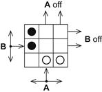
Figure 10-12 An n = 3 Dodgem board.
A and B, in turn, move either of their checkers one square forward (upward for A, rightward for B) or sideways (left or right for A, up or down for B) onto any empty square. Checkers depart the board (permanently) only by a forward move. That player left with no legal move—as a result of being blocked in or having both checkers off the board—wins the game. Each player’s obvious strategic goal is to block his opponent’s progress while pursuing his own.
The deceptively simple 3 × 3 game, invented by Colin Vout (Ref. Vout and Gray), has been strongly solved by Berlekamp, Conway, and Guy (Ref.), proving to be a win for the first player—not surprising, considering the strategy of starting with the outside checker and always keeping it outside. To offset the advantage of moving first, a scoring system has been suggested that awards the winner points corresponding to the number of moves required by the loser to clear the board of his checkers and then subtracting one point.
Appendix Table L details wins and losses for each of the 1332 legal positions. If B plays first, for example, a move from (cf/gh) to any + configuration such as (bf/gh) preserves the winning strategy.
Dodgem obviously offers far greater strategic depth than most other games played on a 3 × 3 matrix (e.g., Tic-Tac-Toe). The 4 × 4 and 5 × 5 games, with optimal play, are never resolved (Ref. desJardins) as both players will repeatedly move their checkers from side to side to block the opponent’s winning move. The percentage of draws increases with increasing n, strongly suggesting that higher-order Dodgem games are also draws with optimal play. (An additional rule advanced for these games designates as the loser that player who prevents his opponent from moving to a position not previously encountered.)
Hex
The inventor of Tac Tix and Soma Cubes, Piet Hein, is also the creator (in 1942) of Hex, an abstract strategy game that shares a distant kinship with Go. (It was independently invented by John Nash9 in 1948.) Hex is played on a rhombic-shaped board composed of hexagons. Conventionally, the Hex board has 11 hexagons along each edge, as shown in Figure 10-13 although any reasonable number can be used (because of the resemblance of the Hex board to the tiles found on bathroom floors, the game is sometimes known as “John”). Two opposite sides of the rhombus are labeled Black, while the other two sides are designated as White; hexagons at the corners of the board represent joint property. Black and white alternately place personal counters on any unoccupied hexagon. The objective for each is to complete a continuous path of personal counters between his two assigned sides of the board.

Figure 10-13 The 11 × 11 Hex board.
It is self-evident that Hex cannot end in a draw, since a player can block his opponent only by completing his own path across the board. There exists a reductio ad absurdum existence proof—similar to that for Tic-Tac-Toe and Gale’s Nim game—that the first player always possesses a win, and complete solutions have been computed for all boards up to and including 9 × 9 Hex (but not for larger boards).
Because the first player has a distinct advantage, the “pie rule” is frequently invoked—that is, the second player is afforded the option of switching positions with the first player after the first counter is emplaced (or after the placement of three counters in some versions). Another method of handicapping allows the second player to connect the shorter width of an n×(n − 1) parallelogram; here, a pairing strategy results in a win for the second player.
The strategic and tactical concepts underlying this seemingly simple game can be quite profound (Ref. Browne). Its solution is inhibited by a large branching factor, about 100, that precludes exhaustive tree-searching (a print-out of the full strategy would be far too unwieldy to be of use).
An interesting analog Hex-playing mechanism (although the game obviously involves digital processes) was designed by Claude Shannon (Ref. 1953) and E.F. Moore. The basic apparatus establishes a two-dimensional potential field corresponding to the Hex board, with White’s counters as positive charges and Black’s as negative charges. White’s sides of the board are charged positively and Black’s negatively. The device contained circuitry designed to locate the saddle points, it being theorized that certain saddle points should correspond to advantageous moves. The machine triumphed in about 70% of its games against human opposition when awarded the first move and about 50% of the time as second player. Its positional judgment proved satisfactory although it exhibited weakness in end-game combinatorial play.
Extending Shannon’s and Moore’s concept, the Hex-playing computer program, Hexy (Ref. Anshelevich), employs a selective α–β search algorithm with evaluation functions based on an electrical-resistor–circuit representation of positions on the Hex board. Every cell is assigned a resistance depending on whether it is empty, occupied by a Black counter, or occupied by a White counter. Electric potentials, applied across each player’s boundaries vary with the configuration of Black and White counters. (Hexy runs on a standard PC with Windows.)
Hexy reaped the Hex tournament gold medal at the 5th Computer Olympiad in London (in 2000). At present, no program can surpass the best human players.
Of the several Hex variants, Chameleon10 offers the greatest interest. Here, Black and White each has the option of placing a counter of either color on the board—and each player wins by connecting a line of either color between his two sides of the board. (If a counter creates a connection between both Black’s and White’s sides (so that all sides are connected), the winner is that player who places the final counter.)
Misère Hex (aka Reverse Hex aka Rex)
Here the object of the game is reversed. White wins if there is a black chain from left to right. Black wins in the event of a white chain from top to bottom.
It has been proved (Ref. Lagarius and Slator) that on an n×n board the first player has a winning strategy for n even, and the second player for n odd. A corollary to this proof confirms that the losing player has a strategy that guarantees every hexagon on the board must be filled before the game ends.
Random-Turn Hex
Rather than alternating turns, the players in this version (Ref. Peres et al.) rely on a coin toss to specify who is awarded the next turn. A computer simulation by Jing Yang has shown that the expected duration of this game on an n × n board is at least n3/2. It is interesting to note that as n becomes large, the correlation between the winner of the game and the winner of the majority of turns throughout the game tends to 0.
Triangular Homeohex11
The field of play consists of a equilateral triangle of side length n packed with n2 equivalent triangles of side length 1. Players alternate in placing a personal computer in any empty cell (unit triangle). The first player to connect all three sides of the triangle wins. Corner cells link to both their adjacent sides. The existence proof for a first-player-win at Tic-Tac-Toe and at Chomp applies equally well to Triangular Hex.
Bridg-it
Superficially similar to Hex is the game of Bridg-It,12 created by David Gale (Ref.). The Bridg-It board, shown in Figure 10-14, comprises an n×(n + 1) rectangular array of dots embedded in a similar n×(n + 1) rectangular array of small blocks (n = 5 in the game originally proposed). In turn, A connects two adjacent dots with an a-colored bridge, and B connects two adjacent blocks with a b-colored bridge. The winner is the player who completes an unbroken line between his two sides of the board.
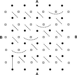
Figure 10-14 The Bridg-It board and Oliver Gross’s solution.
As with Hex, the existence of the first player’s winning strategy is readily proved for Bridg-It. Oliver Gross (Ref. Gardner, 1991) devised the general winning strategy illustrated by the dotted lines in the figure. A begins by playing the bridge indicated in the lower-left corner; thereafter, whenever a bridge by B crosses the end of a dotted line, A plays by crossing the other end of the same line. This pairing strategy—which can be extended to Bridg-It boards of any size—guarantees a win for A.
Double-Move Bridg-It
AfterA’s first move, all subsequent moves for A and B consist of building two bridges.13
Whimsical Bridg-It
At each turn, A or B may build both an a-colored and a b-colored bridge or may choose (at whim) which bridge color to play; the latter option is allowed only once in the game at the cost of a turn. Subsequently, each player builds one bridge of his color per move.14
London Bridg-Its
Each player is restricted to a total of m bridges of his personal color. If neither player has won after the 2m bridges have been placed, the game proceeds by shifting a bridge to a new position at each move.15
Dots and Boxes
This well-known children’s game employs an n×n rectangular grid of dots. Players A and B alternately draw a line connecting any two adjacent dots (horizontally or vertically). Whenever a line completes the fourth side of a square—forming a unit box—the player drawing that line initials that box and draws another line, continuing his turn with each completed box. That player who ultimately initials the greater number of boxes wins the game.
A complete solution for Dots and Boxes has not been determined. Strategic principles, developed by Elwyn Berlekamp (Ref., 2000) recognize the essential parity of the game and underscore its surprising subtleties and mathematical complexities.
Generally, after half (or slightly more) of the 2n(n + 1) possible lines for the n2-box game have been drawn, a state of “gridlock” is reached—that is, the next line must form the third side of at least one box, leaving the next player with one or more boxes to complete before relinquishing his turn. At this stage the grid will have been divided into “chains” (wherein the completion of any one box in the chain leads to the completion of all boxes in the chain).
An inferior but common strategy has the first player after gridlock draw a line conceding the shortest chain. His opponent then concedes the next shortest chain, and so on. If the number of chains at gridlock is even, the player who surrenders the first chain will win (since he will receive an equal or larger chain for his next move); if that number is odd, he will lose (since his opponent claims the last move).
A superior strategy consists of “double dealing”: foregoing the completion of a full chain, accepting instead some fraction of the chain and leaving the remainder for his opponent—thereby gaining control of the game’s progression.
An illustration of this principle, credited to Ian Stewart (Ref., 2001) is shown in the 5×5 game of Figure 10-15—where it is B’s turn to move. Obviously, B will claim the two 2×1 rectangles (B1) in the lower-right and upper-left corners (failure to do so merely surrenders the four boxes to A with no recompense). Now, rather than opening one of the four chains, A executes a double-dealing move by accepting only two of the boxes in the four-box chain (A1), leaving a 2×1 rectangle for B to fill in (B2), after which B is forced to open the five-box chain. A second double-dealing move by A (A2) accepts three of these five boxes, leaves another 2×1 rectangle for B, and forces B to open one of the six-box chains. Thus A has gained control by declining the last two boxes of every chain (except for the last chain).

Figure 10-15 The 5 × 5 Dots-and-Boxes grid.
At gridlock, let ϕ define the number of chains of three-or-more boxes plus the number of dots in the grid. To gain control of the game in the fashion described, A attempts to shape the configuration of lines so that ϕ is even. B, of course, strives to ensure that ϕ is odd.
More Complex Games
Polyominoes
A fascinating class of games can be derived by manipulation of polyominoes on a chessboard (the term polyomino was adopted in 1953 by Solomon W. Golomb, then a graduate student at Harvard University). By definition, an n-omino covers a rookwise-connected set of n squares of the chessboard. Several examples of polyominoes from n = 1 to n = 4 are pictured in Figure 10-16. We can observe that the monominoe and domino have a unique configuration the tromino can assume one of two forms, and the tetromino any of five. Asymmetrical pieces turned over are not regarded as constituting distinct forms.

Figure 10-16 Monomino, domino, trominoes, and tetrominoes.
The general properties of polyominoes have been extensively investigated by Golomb. He has proved a number of theorems, including:
I. The chessboard can be completely covered by 21 straight trominoes and a single monomino if and only if the monomino is placed on one of the four intersections of the 3rd and 6th ranks with the 3rd and 6th files.
II. Regardless of the placement of the monomino, the remaining 63 squares of the chessboard can be covered with 21 right trominoes.
III. The chessboard can be completely covered by 16 straight, square, T-, or L-tetrominoes, but not by 16 skew tetrominoes (in fact, not even a single edge can be completely covered).
IV. It is impossible to cover the chessboard with 15 T-tetrominoes and one square tetromino, nor can coverage be achieved with 15 L-tetrominoes and one square tetromino, nor with 15 straight or skew tetrominoes (in any combination) and one square tetromino.
V. The five distinct tetrominoes cannot be grouped together so as to form an unbroken rectangle.
There exist 12 distinct (“free”) pentominoes—illustrated in Figure 10-17—and named by the letter each most resembles. (Additionally, there are 18 one-sided and 63 fixed pentominoes.) From a recreational standpoint, the properties of pentominoes are more compelling than those of the other polyominoes.

Figure 10-17 The 12 pentominoes.
In Golomb’s Pentomino Game, two players alternately fit onto the chessboard one of the distinct pentominoes until either no pieces remain or none of those remaining will fit on the board. That player unable to place a piece is declared the loser.
Maximum duration of the Pentomino Game is clearly 12 moves—when each of the 12 pieces has been played (a highly improbable situation). Minimum duration is five moves, an example of which is shown in Figure 10-18 none of the remaining seven pentominoes can be placed on the board.

Figure 10-18 A minimal pentomino game.
Golomb propounds two basic strategic principles:
1. Try to move in such a way that there will be room for an even number of pieces.
2. If you cannot analyze the situation, try to complicate the position so that your opponent will have even greater difficulty in analyzing it.
The Pentomino Game was computer-solved by Hilarie K. Orman (Ref.) using a backtracking search procedure and proved to be a win for the first player. There are 296 possible opening moves (2308 without discounting symmetries).
Several variations of the basic game have also been suggested by Golomb. In Choose-Up Pentominoes, the two players alternately select a piece from the set of 12 pentominoes until each has six; the game then proceeds in the normal manner, each player allowed to place only a member of his own set on the board. The player who chooses first plays second to compensate for the advantage of first choice. Strategy for Choose-Up Pentominoes differs from that of the standard game in that instead of attempting to leave an even number of moves following his own move, the player strives to leave as many moves for his own pieces and as few as possible for his opponent’s. An approximate preference ordering of the values of the 12 pentominoes is PNUYLVITZFWX.
In other variations of the basic game, the pentominoes can be distributed at random between the two players, more than one set of the 12 distinct pieces can be used, more than two players can participate, and boards other than the 8 × 8 chessboard can be introduced.
Of the higher-order n-ominoes, the number and complexity increases exponentially with n, rendering them generally unsuitable for game applications. There are, for example, 35 hexominoes and 108 heptominoes, one of the latter being non-simply connected (i.e., its configuration contains a hole). Further, there are 363-octominoes plus six with holes; 1248 enneominoes15 plus 37 with holes; and 4460 decominoes plus 195 with holes. A total of 17,073 hendecominoes16 (Ref. Stein and Ulam) and 63,000 dodecominoes exist, including those multiply connected.
The question of determining the number of distinct n-ominoes as a function of n is identical to a classical unsolved cell growth problem. We consider a square-shaped one-celled animal that can grow in the plane by adding a cell to any of its four sides; we then inquire as to how many distinct connected n-celled animals are possible under isomorphism. Stein, Walden, and Williamson of the Los Alamos Scientific Laboratory have programmed a computer to generate the isomorphism classes of such animals.
Instead of constructing rookwise-connected sets of squares, we can effect the edgewise union of sets of equilateral triangles or of hexagons (only such sets of these three regular polygons can fill a plane). The sets of equilateral triangles, known as polyiamonds, were first explored by T.H. O’Beirne (Ref.). For a given number of cells, fewer distinct shapes are possible than with polyominoes: moniamonds, diamonds, and triamonds can assume only one shape; there are three different-shaped tetriamonds, four pentiamonds, 12 hexiamonds, and 24 heptiamonds.
Solid polyominoes have also been investigated by Golomb and R.K. Guy. Known as “Soma Cubes,” they were invented by the prolific Piet Hein, who conceived the first pertinent theorem: The sole irregular solid tromino and the six irregular solid tetrominoes (irregular in that the figure somewhere contains a corner) can be joined together to fashion a 3 × 3 × 3 cube. These seven solid polyominoes comprise a “Soma set,” which can be used to devise a multitude of entertaining constructions.
Polyominoids
A related set of structures, “polyominoids”—two-dimensional, edge-connected squares in three-space—was originally proposed by the author (Ref. Epstein). An n-ominoid contains n coplanar or orthogonal squares, thus resembling the floors, walls, and ceilings of a pathological office building. There exist two distinct dominoids (one coplanar domino plus one in three-space) and 11 distinct trominoids (two trominoes plus nine in three-space). The number of n-ominoids rises precipitously with increasing n (Table 10-13).
Table 10-13. Number of n-Ominoids

One of the 11 trominoids and four of the 780 pentominoids are illustrated in Figure 10-19 (Ref. www.geocities.com).

Figure 10-19 Polyominoids.
Quadraphage
Initially suggested by the author (Ref. Epstein; Gardner, 1973), the Quadraphage, as its name implies, is a “square-eater”—i.e., a super–chess-like piece that “eats away” whatever square it is placed on. For its move, a q-Quadraphage may consume any q previously uneaten squares on the board.
The Quadraphage may be pitted, in alternating moves, against a chess King—wherein the Quadraphage attempts to entrap the King (which may not traverse an eaten square), preventing it from escaping to the edge of the board.
With q = 1, the King, starting from a position on one of the four central squares of the standard 8 × 8 board, can readily reach an outside square (Ref. Berlekamp, Conway, and Guy, Chapter 19). On boards up to size 33 × 33, the King, with optimal play, cannot be entrapped by the Quadraphage (Ref. Silverman, 1971). On yet larger boards, it is doomed.
As a King versus Quadraphage game, the Quadraphage moves first—with the objective of forcing the King to an edge of the board. The King’s objective is to maximize the number of its moves before reaching an edge. The payoff to the King is one unit for each square obliterated by the Quadraphage, but zero if it becomes entrapped. The game offers yet greater interest when played on the 18 × 18 cells of a Go board.
Postulating a super-King with k = 2 King-moves per turn, it can be proved that such a piece can forever elude the Quadraphage (on an infinite board).
With q = 2 (a second-order Quadraphage), a conventional King cannot escape on boards 8 × 8 and greater. With q = 3, the King can be captured on boards 6 × 6 and greater. And with q = 4 (the Quadraphage obliterates four squares per turn), the King can be trapped on all boards 5 × 5 and greater.
Replacing the King by a Bishop suggests Quadraphage games on an infinite chessboard, but with limitations on the length of the Bishop moves. With q = 3, the Bishop can be captured. Similarly, q = 3 entraps the Rook on an infinite board.
Checkers (Draughts)
Alquerque, the venerable ancestor of Checkers, dates back to 600 B.C. or earlier. Played on a 5 × 5 board, each side controls 12 counters (the center square is initially vacant). About 1100 A.D. in southern France, the game was transferred to a chessboard and titled Dames. Some four centuries later, the French introduced the compulsory-taking rule, referring to the game as Jeu Force. With the 1756 publication of “Introduction to the Game of Draughts” by William Payne, the game rapidly acquired a large following in England and Scotland and soon spread throughout the English-speaking world. It arrived in America, mysteriously renamed Checkers.
In standard 8 × 8 Checkers, seven possible alternatives exist for Black’s opening move, with seven alternative ways of responding. Of the 49 two-move openings, 45 lead to draws and four to losses (with optimal play). There are 144 distinct three-move openings that lead to draws. In major tournaments, players are not allowed to choose opening moves but are assigned an opening selected at random (after eliminating those leading to a loss; each starting position is played twice, with the players exchanging colors for the second game). The preponderant majority of games in expert play are drawn.
With 5 × 10²⁰ positions, Checkers poses a daunting obstacle to any computer attack. The first substantial program was designed in the late 1950s and early 1960s by Arthur L. Samuel of IBM (Ref.). Its principal feature was the introduction of a learning technique enabling the machine to improve its skill with playing experience.
Samuel’s program and its several successors were rendered hors de combat by Chinook, a project that began in 1989 (at the University of Alberta by a team directed by Jonathan Schaeffer) and, with dozens of computers running almost continuously for 18 years, culminated with the complete (weak) solution of Checkers (Ref. Shaeffer et al., 2007). As anticipated, the computational proof determined that the game is a draw.
Chinook’s procedure encompasses three components: (1) an endgame database (backward search) of 3.9 × 10¹³ positions; (2) a proof-tree manager (forward search) that generates positions whose assessment advances the proof’s progress; and (3) a proof solver (forward search) that evaluates each position designated by the manager.
In solving the game of Checkers, this search-intensive (“brute-force”) approach, representing a coupling of AI research and parallel computing, has completed a task six orders of magnitude more complex than achieving, for example, a solution of Connect Four.
It seems likely that the techniques refined by Chinook will be extended to other fields—such as biological processes—where real-time access of immense data sets are of value in accommodating parallel searching.
In its playing prowess, Chinook showed steady improvement from its inception, gaining the title of Checkers World Champion by defeating Dr. Marion Tinsley,17 and then defending its title in subsequent years. It can now claim invincibility, subject only to being tied—well beyond the reach of man or machine.
Checkers Variants
some of the few Checkers variants that have acquired a following:
Brazilian Checkers. Played under the rules of International Draughts, but on an 8 × 8 board with 12 pieces on each side.
Canadian Checkers. International Draughts on a 12 × 12 board with 30 pieces on a side.
Chubby Checkers (suggested by the author). Played on the black squares of a 10 × 10 checkerboard, the 12 pieces of each side are confined to the concentric 8 × 8 playing field. Only Kings are accorded access to the full 10 × 10 board.
International Draughts. Prevalent in Russia and Eastern Europe, often referred to as Polish Draughts (except in Poland, where it is called French Draughts), the game is played on a 10 × 10 board with 20 men per side. It offers commensurately greater complexity (checkers are allowed to capture diagonally backwards, and Kings, known as “Flying Kings,” may travel any number of squares, akin to a chess Bishop that jumps).
Lasca (invented by Emanuel Lasker, former World Chess Champion). Played on a 7 × 7 checkered board with 11 men on each side, 25 diagonally-connected same-colored squares define the playing field. Jumped pieces are placed under the jumper to form a “tower”; only the top piece of a tower may be captured by a jumper.
Suicide Checkers (aka Anti-Checkers, aka Losing Checkers, aka Poddavki). The objective is the opposite of standard Checkers, the winner being that player who loses all his men.
Turkish Checkers (aka Dama in the Middle East). Each player begins with 16 pieces (on the second and third ranks) that move one space straightforward or sideways and capture by jumping over an adjacent opponent piece. At the eighth rank, a piece promotes to a Flying King (Dama) that moves like a chess Rook and may jump over a piece, landing on any empty square beyond.
Chess
Chess (Chaturanga) first appeared in late 6th-century India according to generally accepted but unscholarly sources, confined to a narrow circle of intellectuals. It traveled to Persia about a century later (there known as Shatranj), crossed into Arab culture after a further century, and thence into the western world.
Its Japanese form, Shogi (“General’s Game”), employs a 9 × 9 uncheckered board with 11 pieces and 9 pawns controlled by each player. The Chinese version, Xiangqi (“Elephant Game”), deploys each side’s 11 pieces and 5 pawns on the intersections of 10 horizontal and 9 vertical lines. From its inception, Chess was often regarded with nearly Olympian awe. It still claims supremacy over all other table games, embued with a cryptic mystique—a mystique that, during the middle ages, reached into theological spheres.
Chess rules evolved over nine centuries to 1492, when the Spaniard Ramirez de Lucena introduced castling as a single move, completing what became the modern format. By then the Queen (originally Counselor or Vizier) had augmented its mobility from a King-like one-diagonal-square-at-a-time to become the most powerful figure on the board, and the lowly Pawn was afforded the option of initially advancing two squares (while subject to capture by adjacent pawns en passant).
Chess is a mathematically limited game (comprising a finite number of positions); thus a “perfect” strategy must exist. However, determining this strategy is computationally beyond the pale and will likely remain so failing some revolutionary breakthrough in technology. Such a situation invites computer analysis, and computers now virtually monopolize advances in Chess knowledge. The “silicon beast” flaunts ever more powerful playing programs, databases of hundreds of millions of games, and ever deeper analysis of typical positions.
Chess programs model the game as a tree search wherein each board position corresponds to a node on the game-tree. From the current position each branch represents one of the possible legal moves leading to a new node on the tree, and from each new node further branches lead to other new nodes, et seriatim. The tree is thus made up of alternating levels of moves—known as plys—for either player. (With about 35 moves available from the average position [in mid-game] and with the average game lasting 39 moves, a complete game encompasses more than 10120 potential positions [close to a billion trillion googol], although legal positions number fewer than 1050. Ten thousand high-speed computers, each searching a billion positions a second would wind up woefully short of practicality.)
The groundbreaking game-tree work was formulated in 1950 by Claude Shannon (Ref.), who proposed a playing strategy governed by an evaluation function designed to predict the likely outcome of the game from the current position. The evaluation function need be concerned primarily with strategic knowledge since tactical information is contained essentially in the variations themselves. Shannon’s evaluation function, E, encompassed three factors (material, Pawn structure, and mobility):

where ΔQ, ΔR, ΔB, ΔN, and ΔP are the differences in the number of Queens, Rooks, Bishops, Knights, and Pawns possessed by White over those remaining to Black; ΔD, ΔS, and ΔI represent the differences in doubled Pawns, backward Pawns, and isolated Pawns, respectively; ΔM is the difference in the number of legal moves available.
This function is applied at the terminal nodes of the game tree—that is, at nodes on the level where the search is stopped. A positive value of E defines a position advantageous to White. With White seeking positions that maximize E, and Black countering with positions that minimize E, a minimax solution is theoretically accessible, though Shannon cautioned that such a function—as well as the similar and far more intricate functions that followed in its wake—could claim only “statistical validity.”
Two principal search strategies were (correctly) predicted: Type-A programs that apply “brute force” inspection of every possible position over a fixed number of plys; and Type-B programs that prune potential moves according to some selection function and then examine the significant sets over as many plys as practical and only at those positions reflecting a degree of stability. The apparent weakness of a Type-B strategy is its reliance on the ability to determine which moves in a given situation are worthy of detailed consideration—a problem that proved more intractable than increasing the speed of Type-A searches.
(Shannon also referred to a Type-C program that plays in a manner similar to that of the Chess masters—by evaluation based on learning.)
A third strategy, a quiescence search, was subsequently designed to evaluate tactical concerns such as checking sequences, Pawn promotions, and sequences of capturing moves.
The first Chess-playing program translated into practice was designed by the eminent British theoretician A.M. Turing in 1951 for the MADAM computer. Pursuing an essentially Type-B strategy, the machine performed at a low level of competence, usually resigning after a series of tactical blunders.
A major breakthrough came in 1956 with the introduction, by Prof. John McCarthy at Stanford University, of the alpha-beta algorithm (Ref. Slagle and Dixon), a protocol that eliminates the examination of “any branch that cannot affect the minimax value of the current node,” thereby reducing the branching factor at each node to approximately the square root of the previous value (and doubling the depth of search feasible for a fixed time).
Another technique, known as iterative deepening, also proved of value. Here, a computer performs a series of increasingly deeper searches until its allotted time has expired (as opposed to an exhaustive search of a particular ply). The best move is thereby produced for a given time constraint.
Type-B programs held sway into the 1970s, when improved computational speeds led most investigators to reconsider Type-A programs. By the 1990s, processing power had advanced by several orders of magnitude. With current technology, programs exhaustively search through 10 to 20 ply in the middle game—hundreds of millions of positions per second (early computers enabled a search of about 500 positions per second). Yet, around 1998, Type-B programs staged a comeback, defeating several world-class players over the next few years.
In addition to containing a book of openings with more than a million entries, current Chess programs are linked to a dictionary of endgames, thereby overcoming what had long been a principal weakness owing to the extreme depth of search needed to reach the endgame phase. All six-piece endings have now been analyzed (Ref. Nalimov)—requiring a storage capacity of approximately 1.2 terabytes. (all 5-piece endings require slightly more than seven gigabytes, potentially available to a desktop PC.) A computer reaching one of the positions in an endgame database will be able to continue with perfect play, knowing immediately if its position leads to a win, loss, or draw. Moreover, such knowledge could be useful in either avoiding or steering toward such positions.
Far more sophisticated evaluation functions (Ref. Waters) have been developed since Shannon’s innovation. “Crafty,”18 for example (designed around bitboards, 64-bit data structures), embraces appraisals of the following elements, inter alia:
material; King safety; development of pieces; center control; trapped Rooks; Rooks on open files; doubled Rooks; Rooks behind passed Pawns; trapped Bishops; and isolated, backward, and passed Pawns
Material balance, MB, by far the most significant factor in any evaluation function, is based on relative values compiled in the Chess literature: Queen = 900 points, Rook = 500, Bishop = 325, Knight = 300, Pawn = 100; the King has infinite value. Each side’s MB is then simply the sum of Np, the number of pieces of a certain type still in play, and Vp, the value of that piece: MB = ∑Np Vp.
Assigning relative weights to the various elements comprising the evaluation function is the critical step in determining optimal strategies (Ref. Laramée). A practical limitation on the complexity of the evaluation function lies in the fact that the more time it requires the less time remains for calculating the candidate moves—with a concomitant loss of tactical ability. (At present, it is difficult to enhance an evaluation function to gain as much as can be achieved from an extra ply of search.) This limitation should be alleviated with the advent of greater computer power, an improvement that could also enable nonlinear combinations of the pertinent elements.
The inaugural World Computer-Chess Championship (Stockholm, 1974) was won by the Russian program, Kaissa, a multidomain search process wherein each successive domain examines a subset of moves that were admissible in the preceding domain. Thereafter, the tourney was staged every three years (except for a one-year postponement in 1998) until 2002, when an annual schedule was adopted. The 14th competition (2006) was won by the Israeli program Junior, which analyzes only about three million positions per second but applies highly effective pruning strategies (and can run on a desktop PC).
May 1997 brought the landmark event in human versus machine Chess, when Deep Blue, a complete (Type A) program developed at the IBM Watson Research Center, notched the first match victory over a reigning world champion (Garry Kasparov). Since then, computers such as Rybka (Czech for “little fish”), currently the official (and 15th) World Computer-Chess champion, DEEP JUNIOR, and the supercomputer HYDRA (potentially the strongest Chess engine yet conceived, estimated to warrant an ELO rating19 in excess of 3000), win ever more convincingly over human Chess masters. With a total of 64 gigabytes of RAM, HYDRA can evaluate to a depth of 18 ply. Each of its numerous individual computers incorporates its own field-programmable gate array (FPGA) acting as a Chess co-processor.
With computers thus looming over the chessboard like all-powerful Cyclopses, the demise of classical Chess has become a perennial and oft-lamented prediction among professional Chess masters—although, to the preponderant majority of Chess aficionados, the game still retains (for the foreseeable future) its interest and capacity for creativity.
For world-championship play between humans, a long-standing controversy concerns the manner of scoring draw games. The match comprises 2n games (by custom n = 12) with 1 point awarded for a win, 1/2 point for a draw, and 0 for a loss. The champion requires a score of n points to retain his title; the challenger needs n +  to supersede him.
If champion and challenger are of equal skill, the probability of either winning a single game is  (1 − r), where r is the probability of a draw. Let Rn denote the probability that both score n points. Then the champion will retain his title with probability Pn(r) given by
 (10-3)
The probability Qn(r) that the match will result in k wins by the champion, k wins by the challenger, and 2n − 2k draws is the multinomial distribution (Eq. 2-12),

and

For n = 1, Eq. 10-3 yields
which is minimized for r = 1/3, whence P1(1/3) = 2/3. For n = 2,

which is minimized for r = 0.253, thus yielding P2(0.253) = 0.614. For n = 12, as in championship matches, P12 is minimized with r = 0.087, which yields P12(0.087) = 0.543. The minimizing value of r approaches 0 as n increases.
For moderate values of n, the champion is accorded a substantial advantage by the system that registers draw games as value 1/2; the figures support those who contend that draws should not play a strategic role in championship play. Equation 10-3 advises the champion to play conservatively—that is, to adopt a strategy leading to large values of r—and urges the challenger to seek wins even at considerable risk. In grandmaster play, r∼ 2/3—and the probability that the champion retains his title (against an equally skilled adversary) is P12(2/3) = 0.571. Other values of r produce, as examples, P12(0.9) = 0.635, P12(1/2) = 0.557, and P12(0) = 0.581.
The preceding analysis errs slightly in that champion and challenger can be considered of equal ability only in paired games with each playing White and Black in turn.
Compilations of recent international tournaments indicate that White’s win probability is 0.31, while Black’s is 0.22, leaving 0.47 as the probability of a draw. These data suggest an equitable scoring system of 1 and 0 points to either player for a win and loss, respectively, while White receives 0 and Black is awarded 1/4 point for the draw. Thus, over a series of games, the assignment of the White and Black pieces becomes theoretically irrelevant. For world championship play, drawn games should either be discounted or scored as 1/8 for Black.
Chess Variants
While over 2000 Chess variants have been devised and promoted, only a paltry few have sustained even modest interest from the chess-playing public. Those that are worth noting include the following.
Cheskers. Invented by Solomon Golomb, each player begins with two Kings, a Bishop (equivalent to a Chess Bishop), and a Camel (that lurches one diagonal and two straight squares) on the first rank, and eight Pawns on the second and third ranks. A player must capture all opponent Kings to win.
CHESS960. To address concerns that more and more computer analysis leaves less and less room for originality (virtually all openings have been optimally determined for 20-some moves), Chess960 (aka Fischerandom Chess20) pseudorandomly arranges the starting position of pieces along the first rank. Specifically, the two Bishops are located on opposite colors and can each occupy one of four positions (4 × 4 = 16 permutations); the Queen is placed on one of the remaining six squares (6 choices); the two Knights are placed at random on the remaining five squares [ = 10 possible arrangements)]; on the remaining three empty squares, the King is situated between the two flanking Rooks. This process generates 16 × 6 × 10 × 1 = 960 equiprobable configurations for the starting position. (The order of placement is significant.) Prior to the beginning of each game, one of the 960 configurations is chosen at random, and the contest proceeds with standard rules of play (except for rather complicated castling regulations).
Computers promptly entered the Chess960 lists, oblivious to the irony of engaging in a game designed with “anti-computer” intent. Spike,21 a chess engine22 (not a complete program) developed in Germany, was crowned World Champion at the first Chess960 tournament in 2005 (held in Mainz). It was succeeded the following year by Shredder, another chess program from Germany, one that had previously garnered ten titles as World Computer-Chess Champion.
Crazyhorse. Captured pieces change color and may re-enter the board on any unoccupied square.
Hostage Chess. Captured pieces are held hostage as exchange against the opponent’s captured pieces and then returned to the board.
Kriegspiel. Each player has his own board with the correct positions of his own pieces. The positions of opposing pieces are unknown but deduced. A referee (obviously!) is essential.
Maharajah and the Sepoys. Black has his normal complement of pieces that move conventionally (Pawn promotion and castling are prohibited). White has a single piece, the Maharajah (positioned initially on the King’s square), whose moves combine those of a Queen and a Knight. With perfect play, Black wins.
Suicide (Losing) Chess. Capturing, when possible, is mandatory. The player who loses all his pieces wins.
In general, games with off-beat pieces (unconventional moves) and/or non-standard playing fields remain mired in obscurity.23 The more a proposed variant deviates from classical Chess, the less likely it is to gain popularity.
Go
In contrast to the “artificial” rules that govern Chess and Checkers, the game of Go exhibits a “natural” legalistic structure. It is often described as the most complex game ever devised. As such, it has survived without significant change for over four millennia, its invention traditionally credited to the Chinese emperor Yao.24
With two players alternately setting black and white stones on the intersections of a 19 × 19 grid,25 the deceptively simple objective of Go is (for Black and for White) to form chains of same-colored stones that surround as great an area of the playing field as possible. A vacant point orthogonally adjoining a chain is a degree of freedom, referred to as a liberty; chains or single stones left with no liberties are captured (removed from the board) and added to the opponent’s score at the conclusion of the contest. (Diagonally adjacent stones may cooperate in surrounding territories.) One restriction: the “Ko rule” that prohibits capturing and recapturing moves that lead to immediate repetitive positions. The game is concluded when neither player can increase the number of stones captured or the extent of territories surrounded. Final scoring, then, is the sum of these quantities—albeit to offset Black’s advantage of playing first, an additional 6½ points (komi) is often credited to White’s account.
Go rankings for amateurs delineate a pecking order from 30 kyu (novice) up to 1 kyu and then from 1 dan up to 7 dan. A separate scale applies to professionals, ranging from 1 dan to 9 dan (held by fewer than 200 players worldwide). In a match between two players of unequal rankings, the weaker player is allowed a number of handicap stones equal to the difference between their rankings (these stones are placed on the board at the start of the game).
Six basic concepts shape the general Go strategies:
1. Connectiveness: placing stones in a compact pattern
2. Cutting (isolating) opposing stones
3. Life: creating a pattern of stones that can permanently avoid capture
4. Death: forcing positions wherein opponent stones cannot escape capture
5. Invasion: striving to create a living group within an area controlled by the opponent
6. Reduction: encroaching on opponent’s territory to reduce its size while still maintaining connectiveness
These strategic concepts, in practice, can be highly complex and abstract. Moreover, as the game progresses, it becomes ever more complex (at least for the first 100 plys) as additional stones enter the board—in contrast to most capture games (Chess, Checkers) where positions simplify with time.
Because of its unrivaled strategic depth, its larger board, and an elusive and complex architecture, Go is inherently unamenable both to tree-search and to accurate and practical evaluation functions. Possible position number roughly 3361×0.1252.1×10170, most of which result from about (120!)2 = 4.5 × 10397 different games for a total of 9.3 × 10170 games. By comparison, there are approximately 1080 atoms in the universe. From a typical midgame position, there are about 200 candidate moves; thus a 4-ply search would necessitate examination of 2004 (1.6 × 10⁹) positions. The comparable situation in Chess would entail examination of 354 (1.6 × 10⁶) positions. Further, the average game of Go lasts for some 250 moves, compared to about 39 moves for the average Chess game. A Go computer as powerful as Deep Blue (assessing 500 million positions per second) could not evaluate a single move in a year’s time. The game would seem to defy solution within the foreseeable future.
Initial computer forays focused on reduced board sizes. In 1962, H. Remus developed a Go program for the IBM 704 on an 11 × 11 board, applying the principles of machine learning—weighing the possible number of degrees of freedom of chains, number of stones captured, distance from the last stone set by the opponent, and number and color of stones in certain areas.
An alternative approach combines positional evaluation and tree searching as practiced with Chess. Thorp and Walden (Ref.) have produced such programs for Go on M × N boards with small values of M and N.
Van der Werf et al. (Ref.), applying an iterative deepening alpha-beta search, have produced solutions for all boards up to size 5 × 5.
Other early programs incorporated an “influence function” introduced by Albert Zobrist (Ref.), Black stones are assigned a value of +50, white stones a value of −50, and empty points a zero value. The neighbors of each positive-valued point gain +1 in their influence values and, similarly, the neighbors of negative-valued points tally −1 to their influence values. This process is then repeated another three times, thus “radiating” Black and White influences numerically. The point with the highest value indicates the program’s next move.
Subsequent generations of programs conceptualized abstract representations of the Go board to analyze groupings of stones. Bruce Wilcox (Ref.) developed the theory of sector lines, partitioning the board into zones for individual analysis. Another advance involved pattern recognition to identify typical positions and identify moves—as exemplified by the Goliath program, the 1991 World Computer-Go Champion.
Current Go programs incorporate many of these techniques plus searches on local groups and overall positions, using both patterns and abstract data structures in addition to applying principles of combinatorial game theory, Monte Carlo techniques, and cognitive modeling (cognitive science and Go might be said to share a genetic inheritance). Some programs further emphasize neural networks for candidate-move generation. Databases for full-board openings (fuseki) and corner openings (joseki) are also common features. Yet, with all these elements, even the most proficient Go computers—e.g., Go4+++, Many Faces of Go (written by David Fotland), Go Intellect (1994 Computer-Go Champion), Fungo, Gnugo, and Handtalk—rank about 6 or 7 kyu and pose no threat to accomplished Go players. Handtalk III, developed by Prof. Zhixing Chen at the University of Guangzhou, reigned as World Computer-Go Champion 1995–1997. The current (2006) champion, KCC Igo, along with Handtalk III, were awarded 4-kyu diplomas, still well below the level of professional players.
Programming a computer to play professional-level Go remains a staggeringly complex task. Game theorists predict that, even with Moore’s Law (“Computer power doubles every 18 months”) and a corresponding improvement in search algorithms, such a Go program (shodan) will not be feasible until the early 22nd century. Chaucer’s caveat seems apt: “I warne you well, it is no childes pley.”
Go Variants
Possibly owing to the game’s deep historical roots, Go practitioners tend to view variants prejudicially. The following few can claim some adherents:
DoNotPass Go (suggested by the author). The board is divided into four quadrants (the two mid-line axes are divided between Black and White). Black plays black stones in two diagonally-connected quadrants and white stones in the other two, scoring as Black and White, respectively. White plays the complementary rule.
GoLightly (suggested by the author). Each player may enter either a black or a white stone on the board. Captured pieces of either color are credited to the captor’s account. The player making the last legal move of the game chooses which territory (black- or white-surrounded) to score. GoLightly is usually played on boards smaller than 19 × 19.
Kakomú Go. The edges of the board are lined with Black stones (so White cannot form eyes along an edge). White wins with a group that cannot be captured and loses if all his stones are dead.
No-Go. Each player has the option of rejecting his opponent’s move. The opponent then makes a second move that cannot be rejected.
Phantom Go. Equivalent to Kriegspiel. Each player’s board reflects only his stones and his deductions for the locations of his opponent’s stones. A referee prevents illegal moves. Phantom Go is played more frequently on smaller boards.
Twin Move Go. After Black’s first move, each player is accorded two (independent) consecutive moves.
Games Computers Play
Reversi or Othello (After Shakespeare’s Drama)
Played on an uncheckered 8 × 8 board, this game features 64 checkers that are dark on one side and light on the other. Correspondingly, the two players are designated DARK and LIGHT.
Initially, four counters are placed on the four center squares of the board, two showing light sides and connected diagonally, the other two showing dark sides and also connected diagonally. DARK moves first, placing a counter dark side up in a position that connects directly—either orthogonally or diagonally—to another dark counter and with one or more contiguous light counters between itself and a second dark counter (Figure 10-20). These light counters are then reversed (turned over) to show their dark side. DARK can then use them in subsequent moves unless LIGHT has meanwhile reversed them back.

Figure 10-20 Other starting position.
World championship tournaments for Othello have been held annually since 1977, with Japanese players winning 21 of the 30 contests. Although a strong solution for Othello remains just out of reach (it entails up to 1028 legal positions and a game-tree complexity of about 1058), computer programs such as The Moor and Logistello handily defeat the topmost human players. (Logistello’s evaluation function is based on disc patterns and features over a million numerical parameters that are tuned using linear regression.)
Experts lean to the view that perfectly-played Othello results in a draw (Ref. Allis, 1984).
Connect-Four
a Tic-Tac-Toe–like game played on a vertical board seven columns across and six rows high, Connect-Four pairs two players who begin with 21 counters each of a personal color, alternately placing one on the board. A counter may be entered into a given column only in the lowest unoccupied row of that column. The objective is to achieve a line of four personal counters either orthogonally or diagonally. If all 42 counters have been entered (filling the board) without achieving a line of four, the game is drawn.
Connect-Four has been solved by Victor Allis (Ref., 1988) with a Shannon Type-C program, proving to be a win for the first player.
The Shadow of Things to Come
With the dawn of the 21st century, human versus computer matches have come to be considered as unsporting as human versus automobile races. Computer versus computer will increasingly take over center stage—likely with clusters of computers linked through the Internet, each assigned to search a particular section of the game tree. In 2004, Project ChessBrain set a world record for the largest number of computers (2070) simultaneously playing a game of Chess. (Yet, massively parallel architectures affect only linear increases in computer power—valuable for many games but inadequate for those, like Go, with extremely high complexity.)
Faster hardware and additional processors will steadily improve game-playing program abilities. Computer-memory capacity is increasing exponentially, with a new generation born every three years. Humans, at least for the time being, are constrained by the snail’s pace of biological evolution.
The logical structure of future computers is difficult to forecast. To date, the techniques of game-playing programs have contributed little or nothing to the field of artificial intelligence. Perhaps as a consequence, the present trend is toward an imitation of the human brain structure. Yet a human brain contains approximately 10 billion neurons, logic and memory units, and possesses the capabilities of instinct, intuition, and imagination, which permit intelligent, adaptive, and creative behavior. A contemporary computer, by comparison, encompasses the equivalent of about 100 million neurons; it cannot act intuitively by the accepted meaning of intuition. Human Chess players employ a qualitative and functional analysis; computers might well be advised to seek a different modus operandi.
There is no profound reason why the ultimate format of game-playing computers should resemble a human counterpart any more than interplanetary rockets should adhere to aviary principles. Whatever the course of development, the limits of computers with respect to human functions have yet to be imagined.
Board Bafflers
1. More Numerical Tic-Tac-Toe (Ref. Markowsky, 1990a, 1990b).
Graham’s version. Player A (Odd) owns the set of integers, 1, 3, 5, 7, 9; B (Even) owns 2, 4, 6, 8. Beginning with A, the players alternately place one of their numbers on an empty cell of the standard 3 × 3 matrix. The winner is that player who completes a line—orthogonally or diagonally—whose numbers total 15.
Nygaard’s version. A variation of Graham’s game that additionally awards a win to the player who places any three of his numbers (odd for A, even for B) in a line.
Prove that, with optimal play, Graham’s game is a win for A, while Nygaard’s game is a draw.
2. Plus-or-minus Tic-Tac-Toe. A and B alternately place a number—without replacement—from the set 1, 2, …, 15 on any empty cell of the 3×3 matrix and assign a plus or minus to that number. The winner is the player who completes a line, orthogonally or diagonally, whose numbers sum to zero. Determine the optimal strategies.
3. Knights of the Square Table. How multipronged must a Quadraphage be to entrap two Knights on an n×n board? How much more difficult is it to trap two Knights rather than one?
4. Quadrastructor. To abet his escape from a q-powered Quadraphage, the King engages the services of a Quadrastructor, another super–chess-like piece that can restore an obliterated square or, alternatively, construct a square beyond the original n×n board. (For obvious reasons, the King cannot move onto a new or reconstructed square until its next turn—after the Quadrastructor has leapt to another space.)
Conjecture: To cope with the Quadrastructor (and achieve its stated objective), a q-powered Quadraphage must morph itself into a (q+1)-powered Quadraphage.
5. Show that the total number of squares on an n×n checkerboard is expressed by

6. Versa-Tile Hex. Black’s and White’s counters, if turned over, exhibit the opposite color. For each move, Black/White places a personal counter on any unoccupied hexagon. OR turns over one of his opponent’s counters. A reversed counter cannot to be re-reversed. Show that this game is also a win for the first player.
Allowing a reversed counter to be re-reversed after one or more intervening moves (Vice-versa-Tile Hex) does not alter the basic strategy or outcome of the game.
REFERENCES
Allis LV, van der Meulen M, van den Herik HJ, (1994). Proof-Number Search. Artificial Intelligence.66:91–124.
Allis, L. V., H. J. van den Herik, and M. P. H. Huntjens, “Go Moku Solved by New Search Techniques,” Proceedings 1993 AAAI Fall Symposium on Games: Planning and Learning, 1993.
Allis, Victor, “Search for Solutions in Games and Artificial Intelligence,” Ph.D. Thesis, University of Limburg, Maastricht, 1994.
Allis, Victor, A Knowledge-Based Approach of Connect Four. The Game Is Solved: White Wins, Report IR-163, Faculty of Mathematics and Computer Science, Vrije Universiteit, Amsterdam, Master’s Thesis, October 1988.
Anshelevich Vadim V, (2002). The Game of Hex: The Hierarchical Approach. In: Nowakowski Richard, ed. Games of No Chance. Cambridge University Press: 151–165. .
Arisawa Makoto, (1976–1977). Yashima. Journal of Recreational Mathematics.9(2):133.
Bass U, Fraenkel Aviezri, (1990). The Sprague-Grundy Function for Wythoff’s Game. Theoretical Computer Science.75:311–333.
Berge Claude, Ghouila-Houri A, (1965). Programming, Games and Transportation Networks. Methuen & Co., Ltd.
Berlekamp Elwyn R, Conway John, Guy Richard, (1982). [“The King and the Consumer,” Chapter 19] Academic Press.
Berlekamp Elwyn R, (2000). The Dots and Boxes Game. A. K. Peters [Also in Winning Ways…, pp. 507–550.].
Berliner Hans J, (1973). Some Necessary Conditions for a Master Chess Program. Proceedings of the Third International Joint Conference of Artificial Intelligence.:77–85.
Bernstein Alex, Roberts Michael De V, (1988). Computer v. Chess Player. Computer Chess Compendium. [January].
Bouton Charles, (1901). Nim, a Game with a Complete Mathematical Theory. Annals of Mathematics.3(2):35–39.
Browne Cameron, (2000). Hex Strategy: Making the Right Connections. A. K. Peters.
Byard Stanley, (1950). Robots Which Play Games. Science News.(16):65–77.
Cesare, Gulio, and Henry Ibstedt, “Pebble Game,” Journal of Recreational Mathematics, 2004–2005.
Condon Edward V, (1942). The Nimatron. American Mathematics Monthly.49(5):330–332.
Davies DW, (1950). A Theory of Chess and Noughts and Crosses. Science News.(16):40–64.
desJardins, David, March 1996, www.ics.uci.edu/~eppstein/cgt/dodgem.html .
Domoryad AP, (1961). Matematicheskiye Igri i Razvlecheniya (Mathematical Games and Pastimes). Moscow: Fizmatgiz;.
Epstein Richard A, (1967). The Theory of Gambling and Statistical Logic. Academic Press.
Evans Ronald, (1974). A Winning Opening in Reverse Hex. J. Recreational Mathematics.7(3):189–192.
Evans Ronald J, (1975–1976). Some Variants of Hex. Journal of Recreational Mathematics.8:120–122.
Ferguson, Thomas S., “Another Form of Matrix Nim,” Electronic Journal of Combinatorics, 8, No. 2 (2001), www.combinatorics.org.
Fraenkel Aviezri, (2007). The Raleigh Game. INTEGERS: Electronic Journal of Combinatorics Number Theory.7(2):A13 [1–11.]
Fraenkel Aviezri, (1998). Heap Games, Numeration Systems and Sequences. Annals of Combinatorics.2:197–210 [September].
Fraenkel Aviezri, (1982). How to Beat Your Wythoff Games’ Opponent on Three Fronts. American Mathematics Monthly.89:353–361.
Fraenkel Aviezri, Borosh I, (1973). A Generalization of Wythoff’s Game. Journal of Combinatorics Theory A.15:175–191.
Fraenkel Aviezri, Zusman Dimitry, (2001). A New Heap Game. Theoretical Computer Science.252(1–2):5–12.
Funkenbusch William, Eagle Edwin, (1944). Hyperspacial Tit-Tat-Toe or Tit-Tat-Toe in Four Dimensions. National Mathematics Magazine.19(3):119–122.
Gale D, Neyman A, (1982). Nim Type Games. International Journal of Game Theory.11:17–20.
Gale David, (1974). A Curious Nim-Type Game. American Mathematics Monthly.81(8):876–879.
Gardner Martin, (1959). The Scientific American Book of Mathematical Puzzles and Diversions. Simon and Schuster.
Gardner Martin, (1961). The Second Scientific American Book of Mathematical Puzzles and Diversions. Simon and Schuster.
Gardner Martin, (1958). Mathematical Games. Scientific American.199(3):182–188.
Gardner Martin, (1973). Mathematical Games. Scientific American.228(1):111–113.
Gardner Martin, (1974). Mathematical Games: Cram, Crosscram, and Quadraphage: New Games Having Elusive Winning Strategies. Scientific American.230(2):106–108.
Gardner, Martin, “Bridg-It and Other Games,” New Mathematical Games from Scientific American, 1971.
Gasser Ralph, (1994). Solving Nine Men’s Morris. In: Richard Nowakowski, ed. Games of No Chance. Cambridge University Press: 101–113. .
Gillogly James J, (1972). The Technology Chess Program. Artificial Intelligence.3:145–163.
Goff Allan, (2006). Quantum Tic-Tac-Toe: A Teaching Metaphor for Superposition in Quantum Mechanics. American Journal of Physics.74(11):962–973.
Golomb Solmon W, (1964). Polyominoes. Charles Scribner’s Sons.
Golomb Solomon W, (1954). Checker Boards and Polyomintoes. American Mathematics Monthly.LXI(10):675–682.
Golomb Solomon W, (1961). Part I—Dominoes, Pentominoes and Checker Boards. Recreational Mathematics Magazine.:3–11 [August].
Golomb Solomon W, (1961). Part II—Patterns and Polyominoes. Recreational Mathematics Magazine.:3–12 [October].
Golomb Solomon W, (1961). Part III—Where Pentominoes Will Not Fit. Recreational Mathematics Magazine.:3–22 [December].
Golomb Solomon W, (1962). Part IV—Extensions of Polyominoes. Recreational Mathematics Magazine.:7–17 [April].
Golomb Solomon W, (1966). A Mathematical Investigation of Games of Take-Away. Journal of Combinatorics Theory.1(4):443–458.
Golomb Solomon W, Hales Alfred W, (2002). Hypercube Tic-Tac-Toe. In: Nowakowski Richard, ed. More Games of No Chance. Cambridge University Press: 167–182. .
Grossman HD, Kramer David, (1945). A New Match-Game. American Mathematics Monthly.52:441–443 [October].
Grundy PM, (1939). Mathematics and Games. Eureka.2:6–8.
Grundy PM, Smith Cedric AB, (1956). Disjunctive Games with the last Player Losing. Proceedings Cambridge Philosophic Society.52(Part 3):527–533 [July].
Guy Richard K, (1960). Some Additional Recreation, I. NABLA, The Bulletin of the Malayan Mathematical Society.7(3):97–106.
Guy Richard K, Smith Cedric AB, (1956). The G-Values of Various Games. Proceedings of the Cambridge Philosophic Society.52(Part 3):514–526.
Hales Alfred W, Jewett RI, (1963). Regularity and Positional Games. Transactions of American Mathematics Society.106(2):222–229.
Harary Frank, (1960). Unsolved Problems in the Enumeration of Graphs. Publication of the Mathematics Institute of the Hungarian Academy of Science.(5):63–95.
Holladay John C, (1998). Matrix Nim. American Mathematics Monthly.65(2):107–109.
Holladay John C, (1957). [“Cartesian Products of Termination Games,”] Princeton University Press [Study No. 39, pp. 189–200].
Kalme Charles, (1975). Bobby Fischer: An Era Denied. Chess Life Review.30(11):717–729.
Kenyon, J. C., Nim-like Games and the Sprague–Grundy Theory Master’s Thesis, Department Mathematics, University of Calgary, April 1967.
Kotok, A., “A Chess Playing Program,” Memorandum No. 41 of the RLE and MIT Computation Center, 1962.
Lagarias Jeffrey, Sleator Daniel, (1999). Who Wins Misère Hex?. In: Berlekamp E, Rodgers T, eds. The Mathemagician and Pied Puzzler : A Collection in Tribute to Martin Gardner. A.K. Peters: 237–240. .
Laramée, Françoise Dominic, “Programming Part VI: Evaluations Functions,” October 2002, www.gamedev.net/reference/articles/article1208.asp .
Ma, Wei Ji, “Generalized Tic-Tac-Toe,” (2005), www.weijima.com/index.php?option= com_content&view=article&id=11&Itemid=15 .
McIntyre DP, (1942). A New System for Playing the Game of Nim. American Mathematics Monthly.49(1):44–46.
Madachy Joseph, (1969). Pentominoes—Some Solved and Unsolved Problems. Journal of Recreational Mathematics.2(3):181–188.
Markowsky George, (1990a). Numerical Tic-Tac-Toe I. Journal of Recreational Mathematics.22(2):114–123.
Markowsky George, (1990b). Numerical Tic-Tac-Toe. Journal of Recreational Mathematics.22(3):192–200.
Michie Donald H, (1961). Trial and Error. Penguin Science Survey.(Part 2):129–145.
Moore Eliakim H, (1910). A Generalization of the Game Called Nim. Annals of Mathematics Series.2(11):93–94.
Moser Leo, (1948). Solution to Problem E773. American Mathematics Monthly.55:99.
Mott-Smith Geoffrey, (1954). Mathematical Puzzles. 2nd ed. Dover Publications [rev.]
Murray HJR, (1952). A History of Board Games Other Than Chess. Oxford at the Clarendon Press.
Nalimov, E., “Tablebases,” ftp://ftp.cis.uab.edu/pub/hyatt/TB.
O’Beirne Thomas H, (1961). Puzzles and Paradoxes. New Scientist.224:560–561.
Orman Hilarie, (1996). Pentominoes: A First Player Win. In: Nowakowski Richard J, ed. Games of No Chance. Cambridge University Press: 339–344. .
Paul Jerome L, (1978). Tic-Tac-Toe in n Dimensions. Mathematics Magazine.51(1):45–49.
Peres Yuval, Schramm Oded, Sheffield Scott, Wilson David B, (2007). Random-Turn Hex and Other Selection Games. American Mathematics Monthly.:373–387 [May].
Read RC, (1962). Contributions to the Cell Growth Problem. Canadian Mathematics Journal.14(1):1–20.
Redheffer Raymond, (1948). A Machine for Playing the Game Nim. American Mathematics Monthly.55(6):343–350.
Reiter, Harold., “Just the Factors, Ma’am,” Mathematical Log (Mu Alpha Theta), Summer 2002.
Reitman Walter, Wilcox Bruce, (1977). Pattern Recognition and Pattern-Directed Inference in a Program for Playing Go. ACM SIGART Bulletin.(63):83 [June].
Remus H, (1962). Proceedings of the International Federation of Information Processing Congress. [“Simulation of a Learning Machine for Playing Go”] Holland Publishing Co. [62, pp. 192–194, Munich, September 1962].
Ruderman Harry D, (1951). The Game of Tick-Tack-Toe. Mathematics Teacher.44:344–346.
Samuel Arthur L, (1959). Some Studies in Machine Learning, Using the Game of Checkers. IBM Journal of Research and Development.3:210–229 [July].
Scarne John, (1955). Scarne on Teeko. Crown Publishers.
Schaeffer Jonathan, Burch Neil, Björnsson Yngvi, Kishimoto Akihiro, Müller Martin, Lake Robert, Lu Paul, Sutphen Steve, (2005). Solving Checkers. International Joint Conference on Artificial Intelligence.:292–297.
Schaeffer Jonathan, Burch Neil, Björnsson Yngvi, Kishimoto Akihiro, Müller Martin, Lake Robert, Lu Paul, Sutphen Steve, (2007). Checkers Is Solved. Science.317:1518–1522 [September].
Shannon Claude, (1950). Programming a Computer for Playing Chess. Philosophical Magazine, Series 7.41(314):256–275.
Shannon Claude E, (1955). Game-Playing Machines. J. Franklin Institute.260(6):447–453.
Shannon Claude E, (1953). Computers and Automata. Proceedings IRE.41(10):1234–1241.
Silverman David L, (1971). Your Move. McGraw-Hill.
Silverman David L, (1978). The Fibonacci Split. Journal of Recreational Mathematics.10:314–315.
Slagle JR, Dixon JK, (1969). Experiments with Some Programs that Search Game Trees. Journal of the Association of Computing Machinery.16(2):189–207.
Smith Cedric AB, (1968). Compound Games with Counters. Journal of Recreational Mathematics.1(2):67–77.
Steele, Guy,www.gamerz.net/archives/pbmserv-dev199811/msg00002.html .
Stein P, Ulam S, (1955). A Study of Certain Combinatorial Problems Through Experiments on Computing Machines. Proceedings High-Speed Computer Conference.:101–106 [Louisiana State University].
Stewart Ian, (2001). Dots and Boxes for Experts. Scientific American.284:102–103 [January].
Stewart Ian, (2000). Hex Marks the Spot. Scientific American.282(3):100–103.
Thorp Edward O, Walden William E, (1972). A Computer Assisted Study of Go on M × N Boards. Information Sciences.4(1):1–33.
Van der Werf, Eric C. D., AI Techniques for the Game of Go, Dissertation Series No. 2005–2, Universitaire Pers, Maestricht, 2005.
Van der Werf Eric CD, Jaap van den Herik H, Uiterwijk Jos WHM, (2003). Solving Go on Small Boards. ICGA Journal.26(2):92–107.
Vout Colin, Gray G, (1993). Challenging Puzzles. Cambridge University Press.
Waters, Simon, Trying to Beat Chess Computers, http://simonwaters.Technocool.net/Chess.htm .
Wilcox Bruce, (1985). Reflections on Building Two Go Programs. ACM SIGART Bulletin.94:29–43.
Wythoff WA, (1907). A Modification of the Game of Nim. Nieuw Archief voor Wiskunde.7:199–202.
Zobrist, A., “A Model of Visual Organization for the Game of Go,” Spring Joint Computer Conference, 1970, www.geocities.com/jorgeluismireles/polyominoids/?200617 .
Online Encyclopedia of Integer Sequences.http://home.flash.net/~markthom/html/bridg-it.html www.math.uncc.edu/~hbreiter/The%20Secret%20of%20NIM.htm .
Bibliography
Albert Michael H, (2001). The Game of End-Nim. Electronic Journal of Combinatorics.8 [#R1, 1–12.]
Alonso, J., “Blanco o Negro,” Ajedrez Canario, October (1974).
Bell AG, (1972). Games Playing with Computers. George Allen & Unwin.
Bellman Richard, (1964). System Identification, Pattern Recognition and Dynamic Programming. Hughes Aircraft Co. [December Research Report no. 327].
Berge Claude, (1962). The Theory of Graphs. John Wiley & Sons.
Bernstein Alex, Roberts Michael De V, Arbuckle T, Belsky MA, (1961). A Chess Playing Program for the IBM 704. Proceedings of the Western Joint Computer Conference.:157–159 [published by AIEE, March 1961.]
Block HD, (1955). Learning in Some Simple Non-Biological Systems. American Scientist.53(1):59–79.
Botvinnik Mikhail, (1961). Men and Machines at the Chessboard. The Soviet Review.55(2):55–59 [Pt. 1].
Bouwkamp CJ, (1967). Catalogues of Solutions of the Rectangular 3×4×5 Solid Pentomino Problem. Eindhoven: Technische Hogeschool, Department of Mathematics; [July].
Bouzy Bruno, Cazenove Tristan, (2001). Computer Go: An AI Oriented Survey. Artificial Intelligence.132(1):38–103.
Golomb Solomon W, (1964). Replicating Figures in the Plane. The Mathematical Gazette.(366):403–412.
Golomb Solomon W, (1966). Tiling with Polyominoes. Journal of Combinatorial Theory.:280–286.
Fleischer Rudolf, Trippen Gerhard, (2006). Kayles on the Way to the Stars. [Lecture Notes on Computer Science, 3846/2006] Computational Games.:232–245.
Golomb Solomon W, (1964). Replicating Figures in the Plane. The Mathematical Gazette.366:403–412.
Golomb Solomon W, (1966). Tilling with Polyominoes. Journal of Combination Theory.:280–286.
Guy Richard, (1989). Fair Game. 2nd ed. COMAP.
Hayward Ryan B, van Rijswijck Jack, (2006). Hex and Combinatorics. Discrete Mathematics.306(19–20):2515–2528.
Holshouser Arthur, Reiter Harold, (2001). A Nim-Like Game on the Integers. Mathematics and Informatics Quarterly.11:174–175.
Holshouser Arthur, Reiter Harold, (2005). Misère Games. Mathematical Mayhem.:211–214 [May].
Holshouser, Arthur, and Harold, Reiter, “Abstract: Nim with Twists,” Electronic Journal of Combinatorial Number Theory, www.math.uncc.edu/~hbreiter/NimTwist.pdf.
Holshouser Arthur, Reiter Harold, Rudzinski James, (2003). Dynamic One-Pile Nim. The Fibonacci Quarterly.41(3):253–262.
Irving Geoffrey, Donkers Jeroen, Uiterwijk Jos, (2000). Solving Kalah. ICGA Journal.23(3):139–147.
Kloster Oddvar, (2007). A Solution to the Angel Problem. Theoretical Computer Science.389(Issues 1–2):152–161.
Levy DNL, ed. Complete Chess Compendium. Springer-Verlag.
Lim Chu-Wei, (2005). Partial Nim. Electronic Journal of Combinatorial Theory.G02:1–9 [April].
Marsland TR, Schaeffer Jonathan, eds. Computers, Chess, and Cognition. Springer-Verlag.
Máthé András, (2007). The Angel of Power 2 Wins. Combinatorics, Probability and Computing.15(3):363–374.
Newborn Monroe, (1975). Computer Chess. Academic Press.
Newell Allen, Shaw JC, Simon HA, (1958). Chess Playing Programs and the Problem of Complexity. IBM Journal of Research and Development.2(4):320–335.
Pelikán Pavel, (1962). Machine Performing the Game Nim. Stroje na Zpracování Informací.(8):163–169.
Propp Jim, (1994). A New Take-Away Game. In: Guy Richard, Woodrow Robert E, eds. The Lighter Side of Mathematics. Mathematical Association of America.
Schaeffer Jonathan, (2000). The Games Computers (and People) Play. In: Zelkowitz M, ed. Advances in Computers 50. Academic Press: 189–266. .
Sibert WL, Conway John, (1992). Mathematical Kayles. International Journal of Game Theory.20:237–246.
Slagle James, (1971). Artificial Intelligence: The Heuristic Programming Approach. McGraw-Hill.
Stevens Arthur A, (1969). Bluebook of Charts to Winning Chess. A. S. Barnes & Co.
Sun Xinyu, (2005). Wythoff’s Sequence and N-Heap Wythoff’s Conjectures. Discrete Mathematics.300:180–195 [September].
Weisstein, Erik W., “Rep-tile,” http://mathworld.wolfram.com/Rep-tile.html .
Wichmann Hans, Wichmann Siegfried, (1965). Chess: The Story of Chesspieces from Antiquity to Modern Times. Paul Hamlyn.
1The 3 × 3 game is sufficiently simple that bright chimpanzees have learned to play with creditable performance. Indeed, some casinos have offered the opportunity to compete against trained chickens.
2Analyzed independently by Solomon Golomb and Robert Abbott.
3Marketed under the name Qubic.
4It is also possible to develop the theory with a quaternary representation of the numbers. Such a procedure, although less familiar than binary representation, involves fewer terms.
5A Copenhagen resident of Dutch ancestry, Herre Hein is also the creator of Hex.
6The succeeding analysis of single-pile games was first outlined in a USC lecture by Professor Solomon Golomb.
7Initially proposed by P.M. Grundy.
8“A Midsummer Night’s Dream”: Titania, Queen of the Faeries, laments, “The nine men’s morris is fill’d up with mud, …”
9Nobel laureate in Economics, 1994 (shared with game theorists Reinhard Selten and John Harsanyi).
10Invented independently by Randy Cox and Bill Taylor.
11Suggested by Claude Shannon.
12A trade name marketed by Hasenfield Bros., Rhode Island.
13Invented independently by Randy Cox and Bill Taylor.
14Suggested by Mark Thompson.
15Suggested by the author.
16“Polyominoes” constitutes a false etymology from “dominoes.” Purists would advocate applying strictly Greek-root prefixes rather than the usual deplorable practice of successively mixing Greek and Latin roots.
17Unchallenged as the greatest Checker player ever, Dr. Tinsley held the World Championship for over 40 years, losing only five games in that period. Then along came a computer that was even astuter…
18Written by Bob Hyatt, Crafty is a descendant of Cray Blitz, winner of the 1983 and 1986 World Computer-Chess Championships.
19The standard scale to assess relative strength of tournament Chess players (after its creator, Árpad Élö). Only 39 humans have ever achieved a rating over 2700; only four have surpassed 2800.
20Invented in 1996 by ex-World Champion, turncoat, and notorious anti-Semite, Bobby Fischer.
21After a character in the “Buffy the Vampire Slayer” TV series.
22Computer chess programs are mostly divided into an engine (that computes the best move given a specific position) and, separately, a user interface. The two parts communicate via a communication protocol such as Xboard/Winboard or UCI (Universal Chess Interface).
23More than 1200 different pieces with non-orthodox moves, aka “fairy pieces,” have been invented for the countless concoctions of “fairy Chess.”
24Known as Wei-ch’i (“Envelopment Game”) in Chinese, Go was introduced into Japan around mid-8th century when the Japanese ambassador to China, Kibidaijin, returned home to spread the word.
25Oddly, the Go board is not square. Its grid, for reasons known only to the inscrutable Japanese, has a length-to-width ratio of 15 to 14 (1.5 shaku long by 1.4 shaku wide; one shaku is about 30.3 cm.); margins are added to accommodate stones along the edges. Further, black stones are slightly larger than white stones.