We are surrounded by strings. Strings of bits make integers and floating-point numbers. Strings of digits make telephone numbers, and strings of characters make words. Long strings of characters make web pages, and longer strings yet make books. Extremely long strings represented by the letters A, C, G and T are in geneticists’ databases and deep inside the cells of many readers of this book.
Programs perform a dazzling variety of operations on such strings. They sort them, count them, search them, and analyze them to discern patterns. This column introduces those topics by examining a few classic problems on strings.
Our first problem is to produce a list of the words contained in a document. (Feed such a program a few hundred books, and you have a fine start at a word list for a dictionary.) But what exactly is a word? We’ll use the trivial definition of a sequence of characters surrounded by white space, but this means that web pages will contain many “words” like “<html>”, “<body>” and “ ”. Problem 1 asks how you might avoid such problems.
Our first C++ program uses the sets and strings of the Standard Template Library, in a slight modification of the program in Solution 1.1:
int main(void)
{ set<string> S;
set<string>::iterator j;
string t;
while (cin >> t)
S.insert(t);
for (j = S.begin(); j != S.end(); ++j)
cout << *j << "\n";
return 0;
}
The while loop reads the input and inserts each word into the set S (by the STL specification, duplicates are ignored). The for loop then iterates through the set, and writes the words in sorted order. This program is elegant and fairly efficient (more on that topic soon).
Our next problem is to count the number of times each word occurs in the document. Here are the 21 most common words in the King James Bible, sorted in decreasing numeric order and aligned in three columns to save space:
the 62053 shall 9756 they 6890
and 38546 he 9506 be 6672
of 34375 unto 8929 is 6595
to 13352 I 8699 with 5949
And 12734 his 8352 not 5840
that 12428 a 7940 all 5238
in 12154 for 7139 thou 4629
Almost eight percent of the 789,616 words in the text were the word “the” (as opposed to 16 percent of the words in this sentence). By our definition of word, “and” and “And” have two separate counts.
These counts were produced by the following C++ program, which uses the Standard Template Library map to associate an integer count with each string:
int main(void)
{ map<string, int> M;
map<string, int>::iterator j;
string t;
while (cin >> t)
M[t]++;
for (j = M.begin(); j != M.end(); ++j)
cout << j->first <<" "<< j->second << "\n";
return 0;
}
The while statement inserts each word t into the map M and increments the associated counter (which is initialized to zero at initialization). The for statement iterates through the words in sorted order and prints each word (first) and its count (second).
This C++ code is straightforward, succinct and surprisingly fast. On my machine, it takes 7.6 seconds to process the Bible. About 2.4 seconds go to reading, 4.9 seconds to the insertions, and 0.3 seconds to writing the ouput.
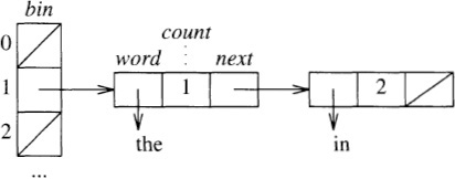
We can reduce the processing time by building our own hash table, using nodes that contain a pointer to a word, a count of how often the word has been seen, and a pointer to the next node in the table. Here is the hash table after inserting the strings “in”, “the” and “in”, in the unlikely event that both strings hash to 1:
We’ll implement the hash table with this C structure:
typedef struct node *nodeptr;
typedef struct node {
char *word;
int count;
nodeptr next;
} node;
Even by our loose definition of “word”, the Bible has only 29,131 distinct words. We’ll follow the old lore of using a prime number near that for our hash table size, and the popular multiplier of 31:
#define NHASH 29989
#define MULT 31
nodeptr bin[NHASH];
Our hash function maps a string to a positive integer less than NHASH:
unsigned int hash(char *p)
unsigned int h = 0
for ( ; *p; p++)
h = MULT * h + *p
return h % NHASH
Using unsigned integers ensures that h remains positive.
The main function initializes every bin to NULL, reads the word and increments the count of each, then iterates through the hash table to write the (unsorted) words and counts:
int main(void)
for i = [0, NHASH)
bin[i] = NULL
while scanf("%s", buf) != EOF
incword(buf)
for i = [0, NHASH)
for (p = bin[i]; p != NULL; p = p->next)
print p->word, p->count
return 0
The work is done by incword, which increments the count associated with the input word (and initializes it if it is not already there):
void incword(char *s)
h = hash(s)
for (p = bin[h]; p != NULL; p = p->next)
if strcmp(s, p->word) == 0
(p->count)++
return
p = malloc(sizeof(hashnode))
p->count = 1
p->word = malloc(strlen(s)+1)
strcpy(p->word, s)
p->next = bin[h]
bin[h] = p
The for loop looks at every node with the same hash value. If the word is found, its count is incremented and the function returns. If the word is not found, the function makes a new node, allocates space and copies the string (experienced C programmers would use strdup for the task), and inserts the node at the front of the list.
This C program takes about 2.4 seconds to read its input (the same as the C++ version), but only 0.5 seconds for the insertions (down from 4.9) and only 0.06 seconds to write the output (down from 0.3). The complete run time is 3.0 seconds (down from 7.6), and the processing time is 0.55 seconds (down from 5.2). Our custom-made hash table (in 30 lines of C) is an order of magnitude faster than the maps from the C++ Standard Template Library.
This little exercise illustrates the two main ways to represent sets of words. Balanced search trees operate on strings as indivisible objects; these structures are used in most implementations of the STL’s sets and maps. They always keep the elements in sorted order, so they can efficiently perform operations such as finding a predecessor or reporting the elements in order. Hashing, on the other hand, peeks inside the characters to compute a hash function, and then scatters keys across a big table. It is very fast on the average, but it does not offer the worst-case performance guarantees of balanced trees, or support other operations involving order.
Words are the basic component of documents, and many important problems can be solved by searching for words. Sometimes, however, I search long strings (my documents, or help files, or web pages, or even the entire web) for phrases, such as “substring searching” or “implicit data structures”.
How would you search through a large body of text to find “a phrase of several words”? If you had never seen the body of text before, you would have no choice but to start at the beginning and scan through the whole input; most algorithms texts describe many approaches to this “substring searching problem”.
Suppose, though, that you had a chance to preprocess the body of text before performing searches. You could make a hash table (or search tree) to index every distinct word of the document, and store a list of every occurrence of each word. Such an “inverted index” allows a program to look up a given word quickly. One can look up phrases by intersecting the lists of the words they contain, but this is subtle to implement and potentially slow. (Some web search engines do, however, take exactly this approach.)
We’ll turn now to a powerful data structure and apply it to a small problem: given an input file of text, find the longest duplicated substring of characters in it. For instance, the longest repeated string in “Ask not what your country can do for you, but what you can do for your country” is “ can do for you”, with “ your country” a close second place. How would you write a program to solve this problem?
This problem is reminiscent of the anagram problem that we saw in Section 2.4. If the input string is stored in c[0.. n – 1 ], then we could start by comparing every pair of substrings using pseudocode like this
maxlen = -1
for i = [0, n)
for j = (i, n)
if (thislen = comlen(&c[i], &c[j])) > maxlen
maxlen = thislen
maxi = i
maxj = j
The comlen function returns the length that its two parameter strings have in common, starting with their first characters:
int comlen(char *p, char *q)
i = 0
while *p && (*p++ == *q++)
i++
return i
Because this algorithm looks at all pairs of substrings, it takes time proportional to n2, at least. We might be able to speed it up by using a hash table to search for words in the phrases, but we’ll instead take an entirely new approach.
Our program will process at most MAXN characters, which it stores in the array c:
#define MAXN 5000000
char c[MAXN], *a[MAXN];
We’ll use a simple data structure known as a “suffix array”; the structure has been used at least since the 1970’s, though the term was introduced in the 1990’s. The structure is an array a of pointers to characters. As we read the input, we initialize a so that each element points to the corresponding character in the input string:
while (ch = getchar()) != EOF
a[n] = &c[n]
c[n++] = ch
c[n] = 0
The final element of c contains a null character, which terminates all strings.
The element a[0] points to the entire string; the next element points to the suffix of the array beginning with the second character, and so on. On the input string “banana”, the array will represent these suffixes:
a[0]: banana
a[l]: anana
a[2]: nana
a[3]: ana
a[4]: na
a[5]: a
The pointers in the array a together point to every suffix in the string, hence the name “suffix array”.
If a long string occurs twice in the array c, it appears in two different suffixes. We will therefore sort the array to bring together equal suffixes (just as sorting brought together anagrams in Section 2.4). The “banana” array sorts to
a[0]: a
a[l]: ana
a[2]: anana
a[3]: banana
a[4]: na
a[5]: nana
We can then scan through this array comparing adjacent elements to find the longest repeated string, which in this case is “ana”.
We’ll sort the suffix array with the qsort function:
qsort(a, n, sizeof(char *), pstrcmp)
The pstrcmp comparison function adds one level of indirection to the library strcmp function. This scan through the array uses the comlen function to count the number of letters that two adjacent words have in common:
for i = [0, n)
if comlen(a[i], a[i+1]) > maxlen
maxlen = comlen(a[i], a[i+1])
maxi = i
printf("%.*s\n", maxlen, a[maxi])
The printf statement uses the “*” precision to print maxlen characters of the string.
I ran the resulting program to find the longest repeated string in the 807,503 characters in Samuel Butler’s translation of Homer’s Iliad. The program took 4.8 seconds to locate this string:
whose sake so many of the Achaeans have died at Troy, far from their homes? Go about at once among the host, and speak fairly to them, man by man, that they draw not their ships into the sea.
The text first occurs when Juno suggests it to Minerva as an argument that might keep the Greeks (Achaeans) from departing from Troy; it occurs shortly thereafter when Minerva repeats the argument verbatim to Ulysses. On this and other typical text files of n characters, the algorithm runs in O(n log n) time, due to sorting.
Suffix arrays represent every substring in n characters of input text using the text itself and n additional pointers. Problem 6 investigates how suffix arrays can be used to solve the substring searching problem. We’ll turn now to a more subtle application of suffix arrays.
How can you generate random text? A classic approach is to let loose that poor monkey on his aging typewriter. If the beast is equally likely to hit any lower case letter or the space bar, the output might look like this:
uzlpcbizdmddk njsdzyyvfgxbgjjgbtsak rqvpgnsbyputvqqdtmgltz ynqotqigexjumqphujcfwn 11 jiexpyqzgsdllgcoluphl sefsrvqqytjakmav bfusvirsjl wprwqt
This is pretty unconvincing English text.
If you count the letters in word games (like Scrabble™ or Boggle™), you will notice that there are different numbers of the various letters. There are many more A’s, for instance, than there are Z’s. A monkey could produce more convincing text by counting the letters in a document — if A occurs 300 times in the text while B occurs just 100 times, then the monkey should be 3 times more likely to type an A than a B. This takes us a small step closer to English:
saade ve mw he n entt da k eethetocusosselalwo gx fgrsnoh,tvettaf aetnlbilo fc lhd okleutsndyeoshtbogo eet ib nheaoopefni ngent
Most events occur in context. Suppose that we wanted to generate randomly a year’s worth of Fahrenheit temperature data. A series of 365 random integers between 0 and 100 wouldn’t fool the average observer. We could be more convincing by making today’s temperature a (random) function of yesterday’s temperature: if it is 85° today, it is unlikely to be 15° tomorrow.
The same is true of English words: if this letter is a Q, then the next letter is quite likely to be a U. A generator can make more interesting text by making each letter a random function of its predecessor. We could, therefore, read a sample text and count how many times every letter follows an A, how many times they follow a B, and so on for each letter of the alphabet. When we write the random text, we produce the next letter as a random function of the current letter. The “order-1” text was made by exactly this scheme:
Order-1: 11 amy, vin. id wht omanly heay atuss n macon aresethe hired boutwhe t, tl, ad torurest t plur I wit hengamind tarer-plarody thishand.
Order-2: Ther I the heingoind of-pleat, blur it dwere wing waske hat trooss. Yout lar on wassing, an sit.” “Yould,” “I that vide was nots ther.
Order-3: 1 has them the saw the secorrow. And wintails on my my ent, thinks, fore voyager lanated the been elsed helder was of him a very free bottlemarkable,
Order-4: His heard.” “Exactly he very glad trouble, and by Hopkins! That it on of the who difficentralia. He rushed likely?” “Blood night that.
We can extend this idea to longer sequences of letters. The order-2 text was made by generating each letter as a function of the two letters preceding it (a letter pair is often called a digram). The digram TH, for instance, is often followed in English by the vowels A, E, I, O, U and Y, less frequently by R and W, and rarely by other letters. The order-3 text is built by choosing the next letter as a function of the three previous letters (a trigram). By the time we get to the order-4 text, most words are English, and you might not be surprised to learn that it was generated from a Sherlock Holmes story (“The Adventure of Abbey Grange”). A classically educated reader of a draft of this column commented that this sequence of fragments reminded him of the evolution from Old English to Victorian English.
Readers with a mathematical background might recognize this process as a Markov chain. One state represents each k-gram, and the odds of going from one to another don’t change, so this is a “finite-state Markov chain with stationary transition probabilities”.
We can also generate random text at the word level. The dumbest approach is to spew forth the words in a dictionary at random. A slightly better approach reads a document, counts each word, and then selects the next word to be printed with the appropriate probability. (The programs in Section 15.1 use tools appropriate for such tasks.) We can get more interesting text, though, by using Markov chains that take into account a few preceding words as they generate the next word. Here is some random text produced after reading a draft of the first 14 columns of this book:
Order-1: The table shows how many contexts; it uses two or equal to the sparse matrices were not chosen. In Section 13.1, for a more efficient that “the more time was published by calling recursive structure translates to build scaffolding to try to know of selected and testing and more robust and a binary search).
Order-2: The program is guided by verification ideas, and the second errs in the STL implementation (which guarantees good worst-case performance), and is especially rich in speedups due to Gordon Bell. Everything should be to use a macro: for n = 10,000, its run time; that point Martin picked up from his desk
Order-3: A Quicksort would be quite efficient for the main-memory sorts, and it requires only a few distinct values in this particular problem, we can write them all down in the program, and they were making progress towards a solution at a snail’s pace.
The order-1 text is almost readable aloud, while the order-3 text consists of very long phrases from the original input, with random transitions between them. For purposes of parody, order-2 text is usually juiciest.
I first saw letter-level and word-level order-k: approximations to English text in Shannon’s 1948 classic Mathematical Theory of Communication. Shannon writes, “To construct [order-1 letter-level text] for example, one opens a book at random and selects a letter at random on the page. This letter is recorded. The book is then opened to another page and one reads until this letter is encountered. The succeeding letter is then recorded. Turning to another page this second letter is searched for and the succeeding letter recorded, etc. A similar process was used for [order-1 and order-2 letter-level text, and order-0 and order-1 word-level text]. It would be interesting if further approximations could be constructed, but the labor involved becomes enormous at the next stage.”
A program can automate this laborious task. Our C program to generate order-k: Markov chains will store at most five megabytes of text in the array inputchars:
int k = 2;
char inputchars[5000000];
char *word[1000000];
int nword = 0;
We could implement Shannon’s algorithm directly by scanning through the complete input text to generate each word (though this might be slow on large texts). We will instead employ the array word as a kind of suffix array pointing to the characters, except that it starts only on word boundaries (a common modification). The variable nword holds the number of words. We read the file with this code:
word[0] = inputchars
while scanf("%s", word[nword]) != EOF
word[nword+l] = word[nword] + strlen(word[nword]) + 1
nword++
Each word is appended to inputchars (no other storage allocation is needed), and is terminated by the null character supplied by scanf.
After we read the input, we will sort the word array to bring together all pointers that point to the same sequence of k words. This function does the comparisons:
int wordncmp(char *p, char* q)
n = k
for ( ; *p == *q; p++, q++)
if (*p == 0 && --n == 0)
return 0
return *p - *q
It scans through the two strings while the characters are equal. At every null character, it decrements the counter n and returns equal after seeing k identical words. When it finds unequal characters, it returns the difference.
After reading the input, we append k null characters (so the comparison function doesn’t run off the end), print the first k words in the document (to start the random output), and call the sort:
for i = [0, k)
word[nword][i] = 0
for i = [0, k)
print word[i]
qsort(word, nword, sizeof(word[0]), sortcmp)
The sortcmp function, as usual, adds a level of indirection to its pointers.
Our space-efficient structure now contains a great deal of information about the k-grams in the text. If k is 1 and the input text is “of the people, by the people, for the people”, the word array might look like this:
word[0]: by the
word[l]: for the
word[2]: of the
word[3]: people
word[4]: people, for
word[5]: people, by
word[6]: the people,
word[7]: the people
word[8]: the people,
For clarity, this picture shows only the first k + 1 words pointed to by each element of word, even though more words usually follow. If we seek a word to follow the phrase “the”, we look it up in the suffix array to discover three choices: “people,” twice and “people” once.
We may now generate nonsense text with this pseudocode sketch:
phrase = first phrase in input array
loop
perform a binary search for phrase in word[0..nword-l]
for all phrases equal in the first k words
select one at random, pointed to by p
phrase = word following p
if k-th word of phrase is length 0
break
print k-th word of phrase
We initialize the loop by setting phrase to the first characters in the input (recall that those words were already printed on the output file). The binary search uses the code in Section 9.3 to locate the first occurrence of phrase (it is crucial to find the very first occurrence; the binary search of Section 9.3 does just this). The next loop scans through all equal phrases, and uses Solution 12.10 to select one of them at random. If the k-th word of that phrase is of length zero, the current phrase is the last in the document, so we break the loop.
The complete pseudocode implements those ideas, and also puts an upper bound on the number of words it will generate:
phrase = inputchars
for (wordsleft = 10000; wordsleft > 0; wordsleft--)
l = -1
u = nword
while 1+1 != u
m = (1 + u) / 2
if wordncmp(word[m], phrase) < 0
1 = m
else
u = m
for (i = 0; wordncmp(phrase, word[u+i]) == 0; i++)
if rand() % (i+l) == 0
p = word[u+i]
phrase = skip(p, 1)
if strlen(skip(phrase, k-1)) == 0
break
print skip(phrase, k-1)
Chapter 3 of Kernighan and Pike’s Practice of Programming (described in Section 5.9) is devoted to the general topic of “Design and Implementation”. They build their chapter around the problem of word-level Markov-text generation because “it is typical of many programs: some data comes in, some data goes out, and the processing depends on a little ingenuity.” They give some interesting history of the problem, and implement programs for the task in C, Java, C++, Awk and Perl.
The program in this section compares favorably with their C program for the task. This code is about half the length of theirs; representing a phrase by a pointer to k consecutive words is space-efficient and easy to implement. For inputs of size near a megabyte, the two programs are of roughly comparable speed. Because Kernighan and Pike use a slightly larger structure and make extensive use of the inefficient malloc, the program in this column uses an order of magnitude less memory on my system. If we incorporate the speedup of Solution 14 and replace the binary search and sorting by a hash table, the program in this section becomes about a factor of two faster (and increases memory use by about 50%).
String Problems. How does your compiler look up a variable name in its symbol table? How does your help system quickly search that whole CD-ROM as you type in each character of your query string? How does a web search engine look up a phrase? These real problems use some of the techniques that we’ve glimpsed in the toy problems of this column.
Data Structures for Strings. We’ve seen several of the most important data structures used for representing strings.
Hashing. This structure is fast on the average and simple to implement.
Balanced Trees. These structures guarantee good performance even on perverse inputs, and are nicely packaged in most implementations of the C++ Standard Template Library’s sets and maps.
Suffix Arrays. Initialize an array of pointers to every character (or every word) in your text, sort them, and you have a suffix array. You can then scan through it to find near strings or use binary search to look up words or phrases.
Section 13.8 uses several additional structures to represent the words in a dictionary.
Libraries or Custom-Made Components? The sets, maps and strings of the C++ STL were very convenient to use, but their general and powerful interface meant that they were not as efficient as a special-purpose hash function. Other library components were very efficient: hashing used strcmp and suffix arrays used qsort. I peeked at the library implementations of bsearch and strcmp to build the binary search and the wordncmp functions in the Markov program.
1. Throughout this column we have used the simple definition that words are separated by white space. Many real documents, such as those in HTML or RTF, contain formatting commands. How could you deal with such commands? Are there any other tasks that you might need to perform?
2. On a machine with ample main memory, how could you use the C++ STL sets or maps to solve the searching problem in Section 13.8? How much memory does it consume compared to McIlroy’s structure?
3. How much speedup can you achieve by incorporating the special-purpose malloc of Solution 9.2 into the hashing program of Section 15.1 ?
4. When a hash table is large and the hash function scatters the data well, almost every list in the table has only a few elements. If either of these conditions is violated, though, the time spent searching down the list can be substantial. When a new string is not found in the hash table in Section 15.1, it is placed at the front of the list. To simulate hashing trouble, set NHASH to 1 and experiment with this and other list strategies, such as appending to the end of the list, or moving the most recently found element to the front of the list.
5. When we looked at the output of the word frequency programs in Section 15.1, it was most interesting to print the words in decreasing frequency. How would you modify the C and C++ programs to accomplish this task? How would you print only the M most common words, where M is a constant such as 10 or 1000?
6. Given a new input string, how would you search a suffix array to find the longest match in the stored text? How would you build a GUI interface for this task?
7. Our program for finding duplicated strings was very fast for “typical” inputs, but it can be very slow (greater than quadratic) for some inputs. Time the program on such an input. Do such inputs ever arise in practice?
8. How would you modify the program for finding duplicated strings to find the longest string that occurs more than M times?
9. Given two input texts, find the longest string that occurs in both.
10. Show how to reduce the number of pointers in the duplication program by pointing only to suffixes that start on word boundaries. What effect does this have on the output produced by the program?
11. Implement a program to generate letter-level Markov text.
12. How would you use the tools and techniques of Section 15.1 to generate (order-0 or non-Markov) random text?
13. The program for generating word-level Markov text is at this book’s web site. Try it on some of your documents.
14. How could you use hashing to speed up the Markov program?
15. Shannon’s quote in Section 15.3 describes the algorithm he used to construct Markov text; implement that algorithm in a program. It gives a good approximation to the Markov frequencies, but not the exact form; explain why not. Implement a program that scans the entire string from scratch to generate each word (and thereby uses the true frequencies).
16. How would you use the techniques of this column to assemble a word list for a dictionary (the problem that Doug McIlroy faced in Section 13.8)? How would you build a spelling checker without using a dictionary? How would you build a grammar checker without using rules of grammar?
17. Investigate how techniques related to k-gram analysis are used in applications such as speech recognition and data compression.
Many of the texts cited in Section 8.8 contain material on efficient algorithms and data structures for representing and processing strings.