Although they didn’t become commonplace in homes until the 1980s, one can’t now imagine a life without computers. The history of the computer is intimately linked with the story of mathematics. We have seen already that pioneers like Leibniz and Pascal blazed (sorry...) a trail with mechanical calculators, but the need for faster and more flexible machines sparked off the digital revolution.
CHARLES BABBAGE (1791–1871)
The English mathematician Charles Babbage was the son of a banker, and is best known as the ‘Father of the Computer’ because of his work in mechanical computing. Babbage read mathematics at Cambridge University but found his studies unfulfilling, which led him to found the Analytical Society in 1812 along with a group of fellow students. Apparently, Babbage’s moment of inspiration came when he was one day poring over a group of logarithm tables that were known to contain many errors. Working out the entries for log tables is a very tricky process and inevitably human ‘computers’ – as they called people who calculated sums in those days – made mistakes. Babbage maintained that the tedious calculations, which require little thought, only accuracy, could be performed by an elaborate calculating machine.
Machine takes over
Babbage secured government funding and produced plans for his Difference Engine. However, such was the complexity and size of the machine that it was never built in his lifetime. (A Difference Engine was built in the 1980s and today resides in London’s Science Museum. At just over 2 metres high and 3.5 metres long it’s a fairly sizeable machine.)
As interest in the Difference Engine project began to wane, Babbage started work on the Analytical Engine using the knowledge he had gleaned while designing his first computer. This machine was intended to be much more like a computer as we know it. It could be programmed to perform particular combinations of mathematical functions. One set of punched cards would be used to programme the engine, another set would introduce data to the engine and then the machine itself could punch blank cards with the results, effectively saving them in its memory for future use.
Babbage was still working on the Analytical Engine when he died. Because of the immense cost and complexity involved, a working model has never been built, although, at the time of writing, British programmer and mathematician John Graham-Cumming is leading a project to build one for the first time.
ADA LOVELACE (1815–52)
One of the few notable pre-twentieth-century female mathematicians, Ada Lovelace was the daughter of the famous poet and rake Lord Byron and Anne Isabella Milbanke, to whom Byron was briefly married. Milbanke was convinced Byron’s excesses had been the result of a kind of insanity and she sought to shield her daughter from a similar fate by encouraging her to pursue a persistent education, especially in the logical discipline of mathematics.
Get with the programme
Despite being unable to enter university, Lovelace was privately tutored and she continued with mathematics throughout her life. She encountered Charles Babbage, who asked her to translate into English an article on his Analytical Engine that had been written by an Italian mathematician. Lovelace duly did so, adding extensive notes on the machine, including a set of instructions that would have had the machine produce the Bernoulli numbers, a sequence of numbers named in honour of Jacob Bernoulli. For this, Lovelace is considered to be the first ever computer programmer. Sadly she died from cancer at the age of thirty-six.
When Ada Lovelace married William King in 1835 she moved to her husband’s estate in Ockham, Surrey, which is believed to have been the birthplace of a monk known as William of Ockham in the late thirteenth century. William of Ockham was a natural philosopher who first coined the principle known as Ockham’s razor: the simplest explanation for a phenomenon more often than not turns out to be true. This principle has been adopted in all scientific fields – when researchers look to explain what they have observed, they try to use existing theories and laws rather than fabricate new ones to fit what they have seen.
GEORGE BOOLE (1816–64)
An Englishman who became a mathematics professor in Ireland, George Boole published major works on differential equations (equations that involve derivatives of a function), but he is most remembered for his work on logic.
Boole sought to set up a system in which logical statements could be defined mathematically and then used to perform mathematical operations on the statements; the results would be generated without the need to think through the problem intellectually. Boole’s system aimed to take a raft of logical propositions and see how they combined together with the aid of maths rather than philosophy.
A logical step
In order to set up the system, Boole developed what became known as Boolean algebra: letters defined either as logical statements or as groups of things. The letters can have a value of 1, meaning ‘true’, and 0, meaning ‘false’.
So imagine you are considering dogs as a group of things, and you let x represent shaggy dogs and y represent yappy dogs. You can then make a table for the dogs using values for x and y:

Boole then defined three simple mathematical operations we could conduct with the results – AND, OR and NOT. AND is defined as the multiple of the two values. As the table below shows, if x and y are ‘true’, we expect the answer ‘true’ or 1, and everything else to be 0 or ‘false’:
This seems rather self-evident – a dog can only be shaggy AND yappy if the dog is shaggy and yappy, but the example is useful because it shows you can come to the same conclusion using very simple arithmetic.
There are a host of other Boolean operations that can be reduced to arithmetic.
In the 1800s Boole’s work had implications for mathematical logic and set theory, but it was not until the twentieth century that a more practical use was found. An electronics researcher called Claude Shannon discovered that he could use Boolean operations in electrical circuits – he could generate a simple electrical circuit to take logical steps and therefore make decisions based on them. As Boole’s work uses only values of 0 or 1, ‘true’ or ‘false’, or ‘on’ or ‘off’ it is known as a digital method. In essence, Boole paved the way for the first electronic digital computers.
Set theory is the branch of mathematics concerned with placing objects into groups called sets. Sets can be defined as containing:
1. numbers (e.g. all odd numbers less than 100)
2. objects (e.g. the set of different types of dogs)
3. ideas (e.g. the set of problems that can be solved by a computer)
Boolean algebra works in set theory, like the example of the shaggy and yappy dogs on page 145.
John Venn (1834–1923) was a British priest and logician who, besides designing and building a cricket-ball-bowling machine, is best known for Venn diagrams, which help to show set theory in a visual way. To use our earlier example, if you are considering all types of dog, then the rectangular box should be receptive to all types of dog. I introduced two sets: x, the set of shaggy dogs and y, the set of yappy dogs. We saw that some shaggy dogs are also yappy, so those two sets need to overlap.
The overlap in the middle represents x AND y. x OR y would be any dog within the two circles. NOT x would be any unshaggy dog.
To bring things back into more mathematical territory, the German mathematician Georg Cantor (1845–1918) was very interested in infinite sets, which, as the name suggests, are sets containing an infinite number of things.
Consider the set of positive whole numbers (1, 2, 3…) which mathematicians call the natural numbers. This is an infinite set because we can keep on counting for ever. Then consider the set of numbers in which the numbers can be anything at all, including fractions, negative numbers and those irrational numbers like π, e and ϕ that we saw earlier (mathematicians call this continuous list of numbers real numbers). This is also an infinite set, and it contains more numbers than the set containing the natural numbers. By comparing the set of natural numbers, which is infinite, with the set of real numbers, which is also infinite, Cantor was able to show that, although both were infinite, they were not the same size. Therefore we have the idea that there are different infinities for different infinite sets. This sort of business is the reason many mathematicians consider infinity to be a concept, rather than a number.
Cantor said that the natural numbers were countably infinite because we make progress towards infinity as we count. The real numbers are uncountably infinite because, no matter where you start counting from, you will not make much progress as you add on an infinitesimal amount each time.
Cantor developed the continuum hypothesis, which states:
There is no set that has more members than the set of integers, but fewer members than the set of real numbers.
So far, it has been proved mathematically that this hypothesis cannot be proved or disproved within the current limits of standard set theory, and it remains one of the greatest unsolved problems in mathematics.
Turing was a brilliant British mathematician and scientist who is well known for the instrumental role he played in the Allied effort to break the German Enigma cipher, a coding machine used by the Nazis during the Second World War.
Memory machine
Prior to the First World War, Turing was a mathematics fellow at Cambridge University. He worked on the Entscheidungsproblem, a challenge set by the German mathematician David Hilbert (see here) that asked whether it is possible to turn any problem in mathematics into an algorithm that will produce a ‘true’ or ‘false’ answer that doesn’t require a proof. Turing was able to show that it is not possible by introducing the concept of an idealized computer called a Turing machine.
A Turing machine is a computer that has an infinite memory that can be fed an infinite amount of data. The machine can then modify the data according to a simple set of mathematical rules to give an output. Turing showed that it was not possible to tell whether a Turing machine would reach an answer to the Entscheidungsproblem, or whether the machine would carry on working out the problem for ever.
The theoretical Turing machine was very important in establishing computer science. Turing’s research into computing took him to Princeton University in the United States, where he worked towards a PhD in mathematics. Here Turing built one of the first electrical computers using Boolean logic (see here), a crucial development towards what came next.
Unpicking the code
Turing was part of the Government Code and Cipher school based at Bletchley Park in Milton Keynes, UK, during the Second World War, where he was set to work on breaking the Enigma cipher. While there Turing developed something called the Bombe, an electro-mechanical machine that could work its way through the huge number of possible settings of the Enigma machine far faster than a human cryptanalyst could. The Bombe relied on the fact that the Enigma would never encrypt a letter as itself – if you typed the letter ‘q’ into the Enigma, ‘q’ wouldn’t be given as an output. The Bombe would try each setting, and when the output letter matched the input letter that setting would be eliminated and the next one tried. The second trick was to use a crib: making an educated guess as to what the first words of an intercepted message might be.
The work of Turing and others at Bletchley Park was hugely important to the Allies and certainly shortened the war. However, the work was top secret and Turing could therefore receive little recognition for his efforts.
Man v machine
After the war Turing continued his work on electronic computers, turning his hand to Artificial Intelligence – whether or not a sufficiently powerful and fast computer could be considered intelligent. During his investigations, Turing devised what has become known as the Turing test. The test states that a computer is to be considered intelligent if a human being communicating with it does not notice that the computer is not a human being. Turing’s work in computers laid the foundations for the digital revolution we now enjoy (and also take for granted). The computer I’m typing this book on, for example, has its origins in a Turing machine.
Into the Chaos
In 1952 Turing turned his hand to biology. In many living things there is a stage when cells change from being very similar to one another to becoming more differentiated. For example, in a developing embryo a group of identical stem cells transform into cells that go into developing the body’s organ system. Turing was able to show that this process, called morphogenesis, is underpinned by simple mathematical rules that, nonetheless, can develop very complex animals. This idea was well ahead of its time and many people thought Turing was wasted on such research. However, many years after his death, his work on morphogenesis would be recognized as the one of the first glimpses of chaos mathematics.
Unfortunately, in 1952 Turing was convicted of gross indecency for homosexual acts, which were deemed illegal at that time. Turing chose to undertake a course of oestrogen injections over a prison sentence. Horrific side effects to the injections led Turing to become depressed, and in 1954 he was found dead of cyanide poisoning. Turing, the founder of modern computing, the unsung war hero, was dead, most likely by his own hand, at the age of forty-one. We can only ponder what discoveries were denied to us by his tragically premature demise.
MAPPING THINGS OUT
Computers were not immediately adopted by mathematicians because many detractors felt that an elegant proof of a problem should be shown formally, rather than by number-crunching. One of the first conjectures proved with the assistance of computing power was called the four-colour theorem.
In the nineteenth century South African mathematician Francis Guthrie (1831–99) was shading in a map of England’s counties when he noticed that each county could be defined from its neighbouring county using just four colours. Guthrie posited this as the four-colour conjecture, which, when put more formally, states that in the instance of a flat two-dimensional map, on which any regions that share a border cannot be the same colour, no more than four colours are ever needed. It is important to note that regions meeting across a point do not share a border and therefore can be the same colour, and that all the countries on the map are independent, so they can be any colour required (unlike the part of Russia where old Königsberg is).

One of the main difficulties with this problem lies in the fact that it is highly visual; there must be an infinite number of maps one could draw to test the theory. However, we can visualize each region as a point using graph theory (much like Euler used with the Königsberg problem).
This allowed mathematicians to start tackling the problem in earnest because various different maps could be shown to have effectively the same graph. Serbian mathematician Danilo Blanusa (1903–87) discovered two maps that needed more than three colours. These elusive maps are known as snarks and they helped to demonstrate that the minimum number of colours required must be four or more. There are eight known snarks, the last of which was discovered in 1989.
In the 1970s two researchers in the United States, Kenneth Appel (1932–) and Wolfgang Haken (1928–), then tackled the four-colour conjecture. They discovered that the most complicated part of any map – any area that might need lots of colours, and which might, therefore, disprove the four-colour conjecture – could always be shown as one of 1,936 possible situations. All of these 1,936 situations could be modelled as a graph and, using a computer, Appel and Haken showed that they could all be drawn using just four colours.
So, Appel and Haken showed that any map could be shown to be one of the 1,936 standard ones, so no counter-examples exist.
This was the first theorem proved with the assistance of a computer, but many mathematicians were unimpressed because the exhaustive proof required hundreds of pages of calculations. This meant that checking the proof would take so long it was necessary to trust that the computer’s work was correct, which was not an assumption many mathematicians would make at the time.
A PIECE OF THE PIE
π, as every schoolchild knows, is a special number that you get by dividing a circle’s circumference (perimeter) by its diameter (the distance across the middle of the circle). Because all circles are mathematically similar (in proportion) you always generate the same value, no matter the size of the circle.
Mathematicians have always been fascinated by π. It is an irrational number (see here) and it is a very useful constant in mathematics that occurs not only in questions about circles but also in all kinds of problems in geometry and calculus. Throughout the history of mathematics we have seen people trying to calculate π to increasing levels of accuracy (see box here). My calculator says:
π = 3.141592654
Since the advent of mechanical and electrical computers, the ability to perform the necessary calculations quickly and accurately has improved exponentially. The Chudnovsky brothers from the USA were the first to get π to 1 billion decimal places using a homemade super-computer in the 1980s. The record is currently owned by Japanese mathematician Yasumasa Kanada, who reached 2.7 trillion (2,700,000,000,000) decimal places in 2010.
Here’s how the value of π has been calculated across the centuries:
In 1900 BC the Ancient Egyptians calculated a value of 256/81 = 3.1605.
The ancient Babylonians had the handier 25/8 = 3.125.
We have inferred from the Bible an approximation of 3.
We saw that Archimedes placed π between 3.1408 and 3.1429, and he also gave us the common school approximation of 22/7.
In China in the fifth century AD, Zu Chongzhi used 355/113 = 3.1415929.
In c. AD 1400 Indian mathematician Madhava calculated 3.1415926539.
The 100 decimal places mark was reached by English astronomy professor John Machin in 1706.
Swiss mathematician Johann Lambert proved π is irrational in 1768.
Chaos theory is the branch of mathematics that deals with unpredictable behaviour. Although this field has really opened up since the advent of computers, chaotic equations were first noticed during Newton’s time.
One of the main aims of Newton’s work was to create a system of equations that explained the motion of the planets. As we know, the planets move around the sun in almost circular orbits. Astronomers had noticed, however, that the orbits would wobble slightly, apparently at random, from time to time.
Leonard Euler (see here) developed a concept that became known as the three-body problem in an attempt to predict the somewhat irregular orbit of the moon. The reason for this irregularity is because the moon’s orbit is influenced by the gravity of both the earth and the sun. The force the sun exerts on the moon varies according to where the moon is in its orbit around the earth, and as a result the moon’s orbit fluctuates. Euler was able to work out the governing equations for the situation in which two of the bodies (the earth and the sun) are in a fixed relationship when compared to the third (the moon). French mathematician Henri Poincaré (1854–1912) tried to extend this to a more general solution that could be applied to the whole solar system. He did not succeed, but he was able to show that the orbits would never settle into a regular pattern.
The motion of the planets was not the only phenomenon scientists had observed to be irregular. The mathematics of turbulence had long eluded mathematicians. When a gas or a liquid flows, the motion of a particle within it can be explained mathematically under certain circumstances – when the speed of the fluid is relatively low. However, as the speed increases, the motion of a particle, particularly around an obstacle, becomes impossible to predict. This turbulence is highly chaotic. The study of the motion of gases and liquids is called fluid mechanics and is important to human beings in all sorts of situations, including transport, electricity generation, and even in understanding the flow of blood around our bodies.
The weather is perhaps the biggest earthly example of turbulence. In the 1960s American meteorologist Edward Lorenz (1917–2008) was modelling the movement of air using a computer when he noticed that, if he changed the initial conditions of his simulations by a negligible amount, as time went by the weather predicted by his simulations would vary widely. This led Lorenz to coin the term ‘the butterfly effect’: the notion that a minuscule change in an air pattern, much like the change induced by a butterfly flapping its wings, could lead to a hurricane happening elsewhere in the world.
It is this sensitivity to initial conditions that causes unpredictable, chaotic behaviour. Even when we completely understand the motion of the particles involved, we can never gather enough detail in our measurements of their speed or mass or temperature to be able to predict an accurate long-term outcome.
The same applies to Turing’s observations in morphogenesis – although the formation of stripes on a zebra is governed by very simple mathematical and chemical rules, immeasurable, tiny differences in each zebra means that they have huge variation in their stripes.
The weather is chaotic – we will never be able to predict it accurately for more than a few days in advance, if that, and even then it is possible that the true outcome could be significantly different than predicted. The Great Storm in Britain in 1987 saw the worst winds for hundreds of years, and yet it was not anticipated.
The computer has been key in the study of chaos mathematics because it allows you to take a model of a situation and run it forward, recalculating the many variables at each stage. Without a computer it can be incredibly time consuming to perform each step, called an iteration. Computers are good for iterative processes, which helps in the next branch of mathematics we shall look at: fractals.
Under the microscope
Although the term ‘fractal’ wasn’t coined until 1975, mathematicians have been fascinated by them for hundreds of years. A fractal is a geometric figure that has what mathematicians call self-similarity: no matter at what scale you look at the image, you still see the same features.
A coastline is a good example of a fractal. Imagine you had a satellite image of a coastline. Without any clues like buildings, trees or boats, you would find it hard to tell whether you were looking at 1,000 miles of coast, or 10 miles of an island. This is because the features – the river inlets, headlands, bays, etc. – look very similar at different scales. The same is true of many features of the natural landscape. Astronauts on the moon found it very hard to gauge the size of boulders – without the haze of atmosphere, they could not tell whether they were looking at a car-sized boulder 100m away or a much larger boulder 500m off.
Everyday Fractals
Many trees and plants have a branching, fractal-like structure. Ferns are especially fractal – the leaves of the plant look exactly like smaller versions of the fronds.
The CGI (computer-generated images) that we enjoy in today’s games and films often use fractal-algorithms to make landscapes, foliage, clouds and even skin and hair look realistic.
Famous fractals
Swedish mathematician Helge von Koch (1870–1924) devised one of the first mathematical fractals, known as the Koch snowflake, which follows a very simple set of rules: you start with an equilateral triangle, and then with each iteration you add another equilateral triangle to the middle third of each line in the diagram. This builds up a snowflake structure as shown:
Besides looking pretty, this snowflake has some very interesting properties. It has the self-similarity property – if you zoom in on an edge you would not be able to tell how many iterations had been performed. If you continued the iterations ad infinitum, the snowflake would have an infinite perimeter even though the snowflake has a finite area.
Polish mathematician Wacław Sierpiński (1882–1969) invented another straightforward geometrical fractal, again based on a triangular theme. For Sierpiński’s triangle, you start with a solid equilateral triangle. You then cut out an equilateral triangle from the middle, which gives you three smaller triangles. At each iteration you cut a triangle out of the middle of any remaining triangles to produce the fractal.
Again, we see self-similarity, as each part of the triangle looks like the whole.
It turns out that there are two other unexpected ways to draw Sierpiński’s triangle. The first harks back to Blaise Pascal and his triangle. If you shade in all the odd numbers in the triangle, you get Sierpiński’s triangle.

The second way is an example of a Chaos Game. You draw the three corners of a triangle and pick a random point inside it. You then, again at random, pick one of the corners of the triangle and move halfway towards it, making a dot at your new position. If you continue this iterative process, you build up Sierpiński’s triangle again! It can take a while by hand, but a computer can do this sort of thing very quickly.

The ultimate fractal
There are many other fractals, but the daddy of them all was created by French-American mathematician Benoit Mandelbrot (1924–2010). As a researcher for the computer company IBM, Mandelbrot was initially interested in self-similarity because he felt it was a common feature of many things, including the stock markets and the way the stars are spread out across the universe. Mandelbrot’s access to the computers at IBM enabled him to perform many iterations quickly, which allowed his studies to thrive. In 1975 he coined the term ‘fractal’.
In the early 1980s he used a computer to investigate for the first time the fractal known as the Mandelbrot set. Like so many of the fractals we have looked at, it has a remarkably simple basis:
This iterative equation says that you get the next number in the sequence, zn+1, by taking the current number zn, squaring it and adding another number, c, to it.
You choose a number, c, and test it using the iteration (starting with z0= 0). Some values of c cause z to get larger and larger, but for others it gets closer and closer to a stable value or else keeps moving around without ever getting larger than 2.
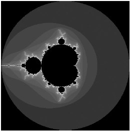
z and c are both complex numbers, which means they have both a real part and an imaginary part (see here). So each value of c has, in effect, two values, which we can plot on a graph as a point. If you plot all the points where c doesn’t ever lead to a value larger than 2, you get an image like this:

If you shade the unstable points on the graphs to indicate how many iterations it took them to become larger than two (the brighter the shade, the more iterations), the famous image emerges.
We can see many self-similar features on the Mandelbrot set, but what is perhaps most amazing is the complexity that arises even though the governing equation is so simple. You can literally zoom into the fractal for ever, a mystery that has led to this fractal assuming the mantle the Thumbprint of God.
As we have seen, the increasing use of computers has also enabled mathematicians to find numeric solutions to equations that cannot be solved using algebra. It is now commonplace for scientists, engineers, designers and inventors to use computer methods to help them in their work. The experiments at the Large Hadron Collider in Europe produce 15 million gigabytes of data each year.
This experiment and many others that require a large amount of number-crunching are now able to exploit the redundant computing power of home computers via the Internet. This distributed computing allows the data to be dealt with far more quickly and allows members of the public to be involved in the frontiers of scientific research.