Timeline Analysis
The amount of time-stamped data available on Windows systems makes timeline analysis a powerful, viable technique for analysts to incorporate into their tool kit. Many times, the cases that we work end up involving some action(s) or events(s) that occurred at a specific time, and understanding timeline creation and analysis can provide valuable insight into system activity that simply cannot be obtained in any other manner. However, as powerful as this technique is, it can still be a very labor-intensive process to collect all of the data that you need, as this technique is based largely on open-source and freeware tools. In this chapter, we will discuss the concepts behind timelines and walk through the process and tools you can use to create timelines for analysis.
Keywords
Timeline; TLN; system activity; time stamp
Information in This Chapter
Introduction
I’ve mentioned several times throughout the book thus far that there are times when commercial forensic analysis applications simply do not provide the capabilities that an analyst may need to fully investigate a particular incident. Despite all of the capabilities of some of the commercial applications, there’s one thing I still cannot do at this point; that is, load an image and push a button (or run a command) that will create a timeline of system activity. Yet the ability to create and analyze timelines has really taken the depth and breadth of my analysis forward by leaps and bounds.
Throughout the day, even with no user sitting at a computer, events occur on Windows systems. Events are simply things that happen on a system, and even a Windows system that appears to be idle is, in fact, very active. Consider Windows XP systems; every 24 hours, a System Restore Point is created, and others may be deleted, as necessary. Further, every three calendar days a limited defragmentation of the hard drive is performed; as you would expect, sectors from deleted files are overwritten. Now, consider a Windows 7 system; Volume Shadow Copies (VSCs) are created (and as necessary, deleted), and every 10 days (by default) the primary Registry hives are backed up. All of these events (and others) occur automatically, with no user interaction whatsoever. So even as a Windows system sits idle, we can expect to see a considerable amount of file system activity over time. When a user does interact with the system, we would expect to see quite a bit of activity: files are accessed, Registry keys and values are created, modified, or deleted, etc. When malware executes, when there is an intrusion, or when other events occur, an analyst can correlate time-stamped data extracted from the computer to build a fairly detailed picture of activity on a system.
Finally, throughout this chapter, we’ll be using tools that I’ve written, and for anyone who knows me, most of my programming over the years has been done in Perl. All of the tools that I wrote and that are listed in this chapter will be available in the online resource, and most of them will be Perl scripts. I’ve also provided them as standalone Windows executable files, or “.exe” files (“compiled” using Perl2Exe); I’ve done this for your convenience. The focus of this chapter is the process of creating timelines; however, if at any point you have a question about a command or what the options are for the command, simply type the command at the command prompt by itself, or follow it with “-h” (for help) or “/?” (also, for help). For most tools, you’ll see the syntax listed with the various options and switches listed; in a few cases, you’ll simply be presented with “you must enter a filename,” which means that the only thing you need to pass to the command is the filename. If, after doing all of this, you still have questions, simply email me.
Timelines
Creating timelines of system activity for forensic analysis is nothing new, and dates back to around 2000, when Rob Lee (of SANS and Mandiant fame) wrote the mac-daddy script to create ASCII timelines of file system activity based on metadata extracted from acquired images using The Sleuth Kit (TSK) tools. However, as time has passed, the power of timeline analysis has been recognized and much better understood. As such, the creation of timelines has been extended to include other data sources besides just file system metadata; in fact, the power of timelines as an analytic resource, using multiple data sources, potentially from multiple systems, is quickly being recognized and timeline analysis is being employed by more and more analysts.
Throughout this chapter, we will discuss the value of creating timelines as an analysis technique and demonstrate a means for creating timelines from an acquired image. The method we will walk through is not the only means for creating a timeline; for example, Kristinn Gudjonsson created log2timeline (found online at http://log2timeline.net/), described as “a framework for [the] automatic creation of a super timeline.” This framework utilizes a number of built-in tools to automatically populate timelines with data extracted from a number of sources found within an acquired image.
This framework can be extremely useful to an analyst. While the approach and tools that I use (which will be described throughout the rest of this chapter) and Kristinn’s log2timeline may be viewed by some as competing approaches, they are really just two different ways to reach the same goal. log2timeline allows for a more automated approach to collecting and presenting a great deal of the available time-stamped data, whereas the tools I use entail a much more command-line-intensive process; however, at the same time, this process provides me with a good deal more flexibility to address the issues that I have encountered.
Data sources
The early days of digital forensic analysis included reviewing file system metadata: metadata which is associated with the time stamps from the $STANDARD_INFORMATION attributes within the master file table (MFT). As we know from Chapter 4, the time stamps within this attribute are easily modified via publicly accessible application programming interfaces (APIs); if you have the necessary permissions to write to a file (and most intruders either get in with or elevate to System-level privileges), you can modify these file times to arbitrary values (this is sometimes referred to as “time stomping,” from the name of a tool used to do this). However, in many cases, rather than “stomping” the file times, the intruder or malware installation process will simply copy the file times from a legitimate system file, such as kernel32.dll, as this is simply much easier to do, requires only a few API function calls, and leaves fewer traces than “stomping” times.
As the Windows operating systems developed and increased in complexity, various services and technologies were added and modified over time. This made the systems more usable and versatile, not only to users (desktops, laptops) but also to system administrators (servers). Many of these services and technologies (i.e., the Registry, application prefetching, scheduled tasks, Event Logs) not only maintain data, but also time stamps which are used to track specific events. Additional services and applications, such as the Internet Information Server (IIS) web server, can provide additional time-stamped events in the form of logs.
As you can see and imagine, Windows systems are rife with timeline data sources, many of which we’ve discussed throughout the book (particularly in Chapter 4). Also, in Chapter 3, we discussed how to get even more time-stamped data and fill in some analytic gaps by accessing VSCs. Overall, Windows systems do a pretty decent job of maintaining time-stamped information regarding both system and user activity. Therefore, it’s critical that analysts understand what data sources may be available, as well as how to access that time-stamped information and use it to further their analysis.
Time formats
Along with the variety of data sources, Windows systems maintain time-stamped information in a variety of formats. The most frequently found format on modern Windows systems is the 64-bit FILETIME format (the structure definition is available online at http://msdn.microsoft.com/en-us/library/ms724284(v=vs.85).aspx) which maintains the number of 100-nanosecond intervals since midnight, January 1, 1601, in accordance with Universal Coordinated Time (UTC—analogous to Greenwich Mean Time (GMT)). As we saw in Chapter 4, this time format is used throughout Windows systems, from file times to Registry key LastWrite times to the ShutdownTime value within the Registry System hive.
Every now and again, you will see the popular 32-bit Unix time format on Windows systems, as well. This time records the number of seconds since midnight on January 1, 1970, relative to the UTC time zone. This time format is used to record the TimeGenerated and TimeWritten values within Windows 2000, XP, and 2003 Event Log records (a description of the structure is found online at http://msdn.microsoft.com/en-us/library/aa363646(VS.85).aspx).
A time format maintained in a great number of locations on Windows systems is the DOSDate format. This is a 32-bit time format, in which 16 bits hold the date and the other 16 bits hold the time. Information regarding the format structure, as well as the process for converting from a FILETIME time stamp to a DOSDate time stamp, can be found at the Microsoft web site (http://msdn.microsoft.com/en-us/library/windows/desktop/ms724274(v=vs.85).aspx). It is important to understand how the time stamps are converted, as this time format can be found in shell items, which themselves are found in Windows shortcut files, Jump Lists (Windows 7 and 8), as well as wide range of Registry data.
Other time-based information is maintained in a string format, similar to what users usually see when they interact with the system or open Windows Explorer, such as “01/02/2010 2:42 PM.” These time stamps can be recorded in local system time after taking the UTC time stamp and performing the appropriate conversion to local time using the time zone and daylight savings settings (maintained in the Registry) for that system. IIS web server logs are also maintained in a similar format (albeit with a comma between the date and time values), although the time stamps are recorded in UTC format.
Yet another time format found on Windows systems is the SYSTEMTIME format (the structure definition is available online at http://msdn.microsoft.com/en-us/library/ms724950(v=vs.85).aspx). The individual elements within the structure of this time format record the year, month, day of week, day, hour, minute, second, and millisecond (in that order). These times are recorded in local system time after the conversion from UTC using the time zone and daylight savings settings maintained by the system. This time format is found within the metadata on Windows XP and 2003 Scheduled Tasks (.job files), as well as within some Registry values, particularly on Vista and Windows 7 (refer to Chapter 5).
Finally, various applications often maintain time stamps in their own time format, particularly in log files. For example, Symantec AntiVirus logs use a comma-separated, text-based format in six hexadecimal octets (defined online at http://www.symantec.com/business/support/index?page=content&id=TECH100099).
So, it’s important to realize that time stamps can be recorded in a variety of formats (to include UTC or local system time), and we will discuss later in this chapter tools and code for translating these time stamps into a common format in order to facilitate analysis.
Concepts
When we create a timeline of system activity from multiple data sources (i.e., more than simply file system metadata), we achieve two basic concepts (credit goes to Cory Altheide for succinctly describing these to me a while back); we add context and granularity to the data that we’re looking at, and we increase our relative level of confidence in that data.
Okay, so what does this mean? Well, by saying that we add context to the data that we’re looking at, I mean that by bringing in multiple data sources, we begin to see more details added to the activity surrounding a specific event. For example, consider a file being modified on the system, and the fact that we might be interested in what may have caused the modification; that is, was it part of normal system activity? Was the file modification part of an operating system or application update (such as with log files)? Or was that file modification the direct result of some specific action performed by a user? By using time-stamped information derived from multiple data sources, normalizing the data (i.e., reducing the time stamps to a common format), and incorporating it into an overall view, we can “see” what additional activity was occurring on the system during or “near” that time. I’ve used timelines to locate file modifications that were the result of a malware infection (see Chapter 6) and could “see” when a file was loaded on a system, and then a short while later the file (i.e., with a “suspicious” name or in a suspicious location) of interest was modified.
How does the term “granularity” fit into a discussion of timelines? When we add metadata from certain data source to our timeline, we can add a considerable amount of details to the timeline. For example, let’s say we start with a timeline that includes file system and Windows Event Log metadata. If we then find a particular event of interest while a user is logged into the system, we can then begin to add metadata specific to that user’s activities to the timeline, including metadata available from historical sources, such as what might be found in any available VSCs. If necessary (depending upon the goals of our analysis) we can then add even more detail, such as the user’s web browsing history, thereby achieving even more granularity. So, separate from context, we can also increase the detail or granularity of the timeline based on the data sources that we include in the timeline, or add to it.
When we say that timelines can increase our relative level of confidence in the data that we’re analyzing, what this means is that some data sources are more easily mutable than others, and we have greater confidence in those that are less easily mutable (or modified). For example, we know that the file time stamps in the $STANDARD_INFORMATION attribute of the MFT can be easily modified through the use of open, accessible APIs; however, those in the $FILE_NAME attribute are not as easily accessible. Also, to this date, I have yet to find any indication of a publicly available API for modifying the LastWrite times associated with Registry keys (remember Chapter 5?) to arbitrary values. These values can be updated to more recent times by creating and then deleting a value within the key, but we may find indications of this activity using tools and techniques described in Chapter 5. The point is that all data sources for our timeline have a relative level of confidence that the times associated with those sources are “correct,” and that relative level of confidence is higher for some data sources (Registry key LastWrite times) than for others (file times in the $STANDARD_INFORMATION attributes of the MFT, log file entries, etc.). Therefore, if we were to see within our timeline a Registry key associated with a specific malware variant being modified on the system and saw that a file also associated with the malware was created “nearby,” then our confidence that the file system metadata regarding the file creation was accurate would be a bit higher.
We also have to keep in mind that the amount of relevant detail available from time-stamped information is often subject to temporal proximity. This is a Star Trek-y sounding term that I first heard used by Aaron Walters (of the Volatility project) that refers to being close to an event in time. This is an important concept to keep in mind when viewing time-stamped data; as we saw in Chapter 4, some time-stamped data is available as metadata contained within files, or as values within Registry keys or values, etc. However, historical information is not often maintained within these sources. What I mean by this is that a Registry key LastWrite time is exactly that; the value refers to the last time that the key contents were modified in some way. What is not maintained is a list of all of the previous times that the key was modified. The same holds true with other time-stamped information, such as metadata maintained within Prefetch files; the time stamp that refers to the last time that particular application was launched is just that—the last time this event occurred. The file metadata does not contain a list of the previous times that the application was launched since the Prefetch file itself was created. As such, it’s nothing unusual to see a Prefetch file (for MSWord, Excel, the Solitaire game, etc.) with a specific creation date, a modification date that is “close” to the embedded time stamp, and a relatively high run count, but what we won’t have available is a list of times and dates for when the application had been previously launched. What this means is that if your timeline isn’t created within relative temporal proximity to the incident, some time-stamped data may be overwritten or modified by activities that occurred following the incident but prior to response activities, and you may lose some of the context that is achieved through the use of timeline analysis. This is an important consideration to keep in mind when performing timeline analysis, as it can explain an apparent lack of indicators of specific activity. I’ve seen this several times, particularly following malware infections; while there are indicators of an infection (Registry artifacts, etc.), the actual malware executable (and often, any data files) may have been deleted and the MFT entry and file system sectors overwritten by the time I was able to obtain any data.
Benefits
In addition to providing context, granularity, and an increased relative confidence in the data that we’re looking at, timelines provide other benefits when it comes to analysis. I think that many of us can agree that a great deal of the analysis we do (whether we’re talking about intrusions, malware infections, contraband images, etc.) comes down to definable events occurring at certain times, respective to and correlated with each other or to some external source. When we’re looking at intrusions, we often want to know when the intruder initially gained access to a system. The same is often true with malware infections; when the system was first infected determines the window of compromise or infection and directly impacts how long sensitive data may have been exposed. With respect to payment card industry (PCI) forensic assessments, one of the critical data points of the analysis is the “window of exposure”; that is, answering the question of when the system was compromised or infected and how long credit card data was at risk of exposure. When addressing issues of contraband images, we may want to know when the images were created on the system in order to determine how long the user may have possessed them, what actions the user may have performed in relation to those images (i.e., launched a viewing application), and when those actions occurred.
These examples show how analysis of timeline data can, by itself, provide a great deal of information about what happened and when for a variety of incidents. Given that fact, one can see how creating a timeline has additional benefits, particularly when it comes to triage of an incident, or the exposure of sensitive data is in question. One challenge that has been faced by forensic analysts consistently over the years has been the ever-increasing size of storage media. I can remember the days when a 20-megabyte (MB) hard drive was a big deal; in fact, I can remember when a hard drive itself was a big deal! Over time, we’ve seen hard drive sizes go from MB to gigabytes (GB) to hundreds of GB, even into terabytes (TB). I recently received a 4-TB hard drive as a reward for winning an online challenge. But storage capacity has not only going up for hard drives, it’s increased for all storage media. External storage media (thumb drives, external hard drives) have at the same time increased in capacity and decreased in price. The same is also true for digital cameras, smart phones, etc.
Where creating timelines can be extremely beneficial when dealing with ever-increasing storage capacity is that they are created from metadata, rather than file contents. Consider a 500-GB hard drive; file system metadata (discussed later in this chapter) extracted from the active file system on that hard drive will only comprise maybe a dozen or so kilobytes (KB). Even as we add additional data sources to our timeline information (such as data from Registry hives, or even the hive files themselves), and the data itself approaches hundreds of KB, it’s all text-based and can be compressed, occupying even less space. In short, the relevant timeline data can be extracted, compressed, and provided or transmitted to other analysts far more easily than transmitting entire copies of imaged media.
In order to demonstrate how this is important, consider a data breach investigation where sensitive data (such as PCI) was possibly exposed. These investigations can involve multiple systems, which require time to image, and then time to analyze, as well as time to search for credit card numbers. However, if the on-site responder were to acquire images, and then extract a specific subset of data sources (either the files themselves or the metadata that we will discuss in this chapter), this data could be compressed, encrypted, and provided to an off-site analyst to conduct an initial analysis or triage examination, all without additional exposure of PCI data, as file contents are not being provided.
The same can be said of contraband image investigations. Timeline data can be extracted from an acquired image and provided to an off-site analyst, without any additional exposure of the images themselves; only the file names and paths are provided. The images themselves do not need to be shared (nor should they) in order to address such questions as how or when the images were created on the system, or whether the presence of the images is likely the result of specific user actions (as opposed to malware). While I am not a sworn law enforcement officer, I have assisted in investigations involving contraband images; however, the assistance I provided did not require me (thankfully) to view any of the files. Instead, I used time-stamped data to develop a timeline, and in several instances was able to demonstrate that a user account had been accessed from the console (i.e., logging in from the keyboard) and used to view several of the images.
In short, it is often not feasible to ship several TB of acquired images to a remote location; this would be obviated by the time it would take to encrypt the data, as well as by the risks associated with the data being lost or damaged during shipment. However, timeline data extracted from an acquired image (or even from a live running system) can be archived and secured, and then provided to an off-site analyst. As an example, I had an image of a 250-GB hard drive, and the resulting timeline file created using the method outlined in this chapter was about 88 KB, which then compressed to about 8 KB. In addition, no sensitive data was exposed in the timeline itself, whereas analysis of the timeline provided answers to the customer’s questions regarding malware infections.
Another aspect of timeline analysis that I have found to be extremely valuable is that whether we’re talking about malware infections or intrusions or another type of incident, in the years that I’ve been performing incident response and digital forensic analysis as a consultant, it isn’t often that I’m able to get access to an image of a system that was acquired almost immediately following the actual incident. In most cases, a considerable amount of time (often weeks or months) has passed before I get access to the necessary data. However, very often, creating a timeline using multiple data sources will allow me to see the artifacts of an intrusion or other incident that still remain on the system. Remember in Chapter 1 when we discussed primary and secondary artifacts? Well, many times I’ve been able to locate secondary artifacts of an intrusion or malware/bot infection, even after the primary artifacts were deleted (possibly by an AV scan, or the result of first responder actions). For example, during one particular engagement, I found through timeline analysis that specific malware files had been created on a system, but an AV scan two days later detected and deleted the malware. Several weeks later, new malware files were created on the system, but due to the nature of the malware, it was several more weeks before the portion of the malware that collected sensitive data was executed (this finding was based on our analysis of the malware, as well the artifacts within the timeline). By locating the secondary artifacts associated with the actual execution of the malware, this allowed us to specify the window of exposure for this particular system to a more accurate and narrow time frame, for which the customer was grateful.
Finally, viewing data from multiple sources allows an analyst to build a picture of activity on a system, particularly in the absence of direct, primary artifacts. For example, when a user logs into a system, a logon event is generated but it is only recorded in the Security Event Log if the system is configured to audit those events. If an intruder gains access to or is able to create a domain administrator account and begin accessing systems (via the Remote Desktop Protocol), and that account has not been used to log into the systems previously, then the user profile for the account will be created on each system, regardless of the auditing configuration. The profile creation, and in particular the creation of the NTUSER.DAT hive file, will appear as part of the file system data, and the contents of the hive file will also provide the analyst with some insight as to the intruder’s activities while they were accessing the system. I’ve had several examinations where I was able to use this information to “fill in the gaps” when some primary artifacts were simply not available.
Format
With all of the time-stamped information available on Windows systems, in the various time stamp structures, I realized that I needed to create a means by which I could correlate all of it together in a common, “normalized” format. To this end, I came up with a five-field “TLN” (which is short for “timeline”) format to serve as the basis for timelines. This format would allow me to provide a thorough description of each individual event, and then correlate, sort, and view them together. Those five fields and their descriptions are discussed below.
Time
With all of the various time structures that appear on Windows systems, I opted to use the 32-bit Unix time stamp, based on UTC as a common format. All of the time stamp structures are easily reduced or normalized to this common format, and the values themselves are easy to sort on and to translate into a human-readable format using the Perl gmtime() function. Also, while Windows systems do contain a few time values in this 32-bit format, I did not want to restrict my timelines to Windows systems only, as in many incidents valuable time-stamped data could be derived from other sources as well, such as firewall logs, network device logs (in syslog format), and even logs from Linux systems. As I did not have access to all possible log or data sources that I could expect to encounter when I was creating this format, I wanted to use a time stamp format that was common to a wide range of sources, and to which other time stamp structures could be easily reduced.
Tools and functions available as part of programming languages make it easy to translate the various time structures to a normalized Unix epoch time UTC format. Most time stamps are stored in UTC format, requiring nothing more than some math to translate the format. Remember, however, that the SYSTEMTIME structure can be based on the local system time for the system being examined, taking the time zone and daylight savings settings into account. As such, you would first need to reduce the 128-bit value to the 32-bit time format, and then make the appropriate adjustments to convert local time to UTC (86,400 seconds/hour times the ActiveTimeBias value from the Registry, for that system, and for that time of year).
Source
The source value within the TLN format is a short, easy-to-read identifier that refers to the data source within the system from which the time-stamped data was derived. For example, as we’ll see later in this chapter, one of the first places we often go to begin collecting data is the file system, so the source would be “FILE.” For time-stamped data derived from Event Log records on Windows 2000, XP, and 2003 systems I use the “EVT” (based on the file extension) identifier in the source field, whereas for Vista, Windows 7, and Windows 8 systems, I use the “EVTX” identifier for events retrieved from the Windows Event Logs on these systems. I use “REG” to identify data retrieved from the Registry, and “SEP” or “MCAFEE” to identify data retrieved from Symantec EndPoint Protection Client and McAfee AV log files, respectively.
You might be thinking, what is the relevance of identifying different sources? Think back to earlier in this chapter when we discussed the relative level of confidence we might have in various data sources. By using a source identifier in our timeline data, we can quickly see and visualize time-based data that would provide us with a greater level of relative confidence in the overall data that we’re looking at, regardless of our output format. For example, let’s say that we have a file with a specific last modified time (source FILE). We know that these values can be modified to arbitrary times, so our confidence in this data, in isolation, would be low. However, if we have a Registry key LastWrite time (source REG) derived from one of the most recently used (MRU) lists within the Registry (such as the RecentDocs subkeys, or those associated with a specific application used to view that particular file type) that occurs prior to that file’s last modified time, we’ve increased our confidence in that data.
I do not have a comprehensive list or table of all possible timeline source identifiers, although I have described a number of the more frequently used identifiers. I try to keep them to eight characters or less, and try to make them as descriptive as possible, so as to provide context to the data within the timeline. A table listing many of the source identifiers that I have used is included along with the materials associated with this book.
System
This field refers to the system, host, or device from which the data was obtained. In most cases within a timeline, this field will contain the system or host name, or perhaps some other identifier (based on the data source), such as an IP address or even a media access control address. This can be very helpful when you have data from multiple sources that describe or can be associated with a single event. For example, if you’re looking at a user’s web browsing activity, you may have access to the user’s workstation, firewall logs, perhaps web server proxy logs, and in some cases, maybe even logs from the remote web server. In other instances, it may be beneficial to combine timelines from multiple systems in order to demonstrate the progression of malware propagating between those systems, or an adversary moving laterally within an infrastructure, from one system to another. Finally, it may be critical to an investigation to combine wireless access point log files into a timeline developed using data from a suspect’s laptop. In all of these instances, you would want to have a clear, understandable means for identifying the system from which the event data originated.
User
The user field is used to identify the user associated with a specific event, if one is available. There are various sources within Windows systems that maintain not just time-stamped data, but also information tying a particular user to that event. For example, Event Log records contain a field for the security identifier (SID) of the user associated with that particular record. In many cases, the user is simply blank, “System,” or one of the SIDs associated with a System-level account (LocalService, NetworkService) on that system. However, there are a number of event records that are associated with a specific user SID; these SIDs can be mapped to a specific user name via the SAM Registry hive, or the ProfileList subkeys from the Software hive.
Another reason to include a user field is that a great deal of time-based information is available from the NTUSER.DAT Registry hive found in each user profile. For example, not only do the Registry keys have LastWrite times that could prove to be valuable (again, think of the MRU keys), but various Registry values (think UserAssist subkey values) also contain time-based data. So, while many data sources (e.g., file system and Prefetch file metadata) will provide data that is not associated with a specific user, adding information derived from user profiles (specifically the NTUSER.DAT hive) can add that context that we discussed earlier in this chapter, allowing us to associate a series of events with a specific user. Populating this field also allows us to distinguish the actions of different users.
Description
This field provides a brief description of the event that occurred. I’ve found that in populating this particular field, brief and concise descriptions are paramount, as verbose descriptions not only quickly get out of hand, but with many similar events analysts will have a lot to read and keep track of when conducting analysis.
So what do I mean by “brief and concise”? A good example of this comes in representing the times associated with files within the file system. We know from Chapter 4 that files have four times (last modified, last accessed, when the file metadata was modified, and the file creation or “born” date) associated with each file, usually derived from the $STANDARD_INFORMATION attribute within the MFT. These attributes are often abbreviated as “MACB.” As such, a concise description of the file being modified at a specific time would be “M…<filename>.” It’s that simple. The “M” stands for “modified,” the dots represent the other time stamps (together they provide the “MACB” description), and the filename provides the full path to the file. This is straightforward and easy to understand at a glance.
I have found that doing much the same thing with Registry LastWrite times is very useful. Listing the key name preceded by “M…,” much like last modified times for files, is a brief and easy-to-understand means for presenting this information in a timeline. Registry key LastWrite times mark when a key was last modified, and by itself, does not contain any specific information about when the key was created. While it’s possible that the LastWrite time also represents when the key was created, without further contextual information, it is best not to speculate and to only consider this value “as is”—that is, simply as the LastWrite time.
When populating at timeline with Event Log records, I’ve found that a concise description can be derived from elements of the event itself. Using the event source from the Event Log record, along with the event identifier (ID), the type (warning, info, or error), and the strings extracted from the event (if there are any), I’ve been able to create a brief description of the event. For example, on Windows XP and 2003 systems, event ID 520 (source is “Security”) indicates that the system time had been successfully changed; from such an event record, the Description field would appear as follows:
Security/520;Success;3368,C:\WINDOWS\system32\rundll32.exe,vmware, REG-OIPK81M2WC8,(0×0,0×91AD),vmware,REG-OIPK81M2WC8,(0×0,0×91AD), 1/17/2008,4:52:28 PM,1/17/2008,4:52:27 PM
To understand what each of the fields following “Security/520;Success;” refers to, see the event description found online at http://www.ultimatewindowssecurity.com/securitylog/encyclopedia/event.aspx?eventid=520. A Description field such as the above example might seem a bit cryptic at first to some analysts, but over time and looking at many timelines, I’ve developed something of an eye for which events to look for when conducting analysis. In addition, I’ve relied heavily on the EventId.net web site, purchasing a new subscription every year so that when the next exam comes up I can search for and review the details of the various event sources and IDs.
TLN format
Now that we’ve discussed the five basic fields that can comprise a timeline, you’re probably asking yourself, “Okay, in what format are these events stored?” I have found that storing all of these events in an intermediate “events” file (usually named “events.txt”) in a pipe (“|”) delimited format makes them very easy to parse (we will discuss parsing the events file later in the chapter). As such, each individual event appears as follows in the events file:
The use of a pipe as a separator was a pretty arbitrary choice, but I needed to use something that wasn’t likely to show up in the Description field (like a comma or semicolon) and play havoc with my parsing utility. The pipe seemed like a pretty good choice.
Creating Timelines
With all this talk about timelines, it’s about time we created one. What we’ll do is walk through a demonstration of creating a timeline from a Windows XP image, start to finish, pointing out along the way different techniques for getting similar information from Vista and Windows 7 systems, as well as some alternative techniques for obtaining the same information.
This process is going to be modular in nature, allowing us a great deal of flexibility in creating timelines. As we walk through the process, you’ll notice that we’re creating the timeline in stages. In some of the steps, the data that we extract will be stored in an intermediate file. We will first extract the data into an intermediate file in one format (generally whatever format is used by the tool capable of extracting our data of interest). We’ll then use another tool to manipulate that data into a normalized format (TLN format) in an intermediate “events” file. Since our events file will contain multiple sets of unsorted data appended to the file, our last step will be to parse the events file and sort it into a final timeline. This can be very beneficial, particularly if an application uses a new format to store its data, or something happened with the application that corrupted the data that we’re parsing—think of this as something of a debugging step, as checking the contents of the intermediate file can help you figure out whether something wrong, and how to fix it. Remember, there are no commercial forensic analysis applications that allow us to press a button and create timelines from all available data; rather, we often have to rely on multiple open-source and freely available tools to extract the necessary data. As these tools are often created by various authors with completely disparate goals in mind, we often have to extract the data into the format provided by the tool, and then manipulate or restructure the data so that we can add it more easily to our timeline format.
So, starting with an acquired image, we will extract the data we want or need in whatever format is provided by the available tools, and then use or create the necessary tools to put that data into our common timeline format in an “events” file, which we will then parse into a timeline. I know that this process does seem terribly manual and perhaps cumbersome at first, but to be honest, over time I’ve found that having this sort of granular level of control over the information that is added to a timeline can be advantageous. However, once you’ve walked through this process once or twice and seen the value of creating a timeline, seeing the perspective that you can get on a case by viewing different and apparently disparate system events correlated together, you’ll recognize the power that a timeline can bring to the analyst. Hopefully, through the course of our discussion, you will see just how powerful an analysis technique creating a timeline can be and take the opportunity to use it.
Before we get started, we need to make sure that we have the necessary tools available. The process that we will be discussing makes use of Perl scripts that I have written; those scripts are available in the materials associated with this book, and include executable files “compiled” using Perl2Exe, so that a Perl distribution does not need to be installed in order to use the tools. In addition to these tools, you will need TSK tools, which can be found online at http://www.sleuthkit.org/sleuthkit/download.php. Once you’ve assembled this collection of tools, you will be ready to start creating timelines.
Do not feel that you are necessarily limited by the process that we’re about to discuss; rather, look at it as an introduction. If you have a favorite tool that provides data that you’d like to add to your timeline, feel free to use it. The process that we’re going to discuss should simply be considered a foundation, in order to provide an understanding of where the data comes from, and how it can be used to build a timeline.
As we’re going to be creating a timeline from an acquired image, you will need to have an image available so that you can follow along with and use the commands that comprise the process that we will walk through in the rest of this chapter. There are a couple of ways to obtain an image of a Windows system if you don’t already have one—one is to simply use FTK Imager to acquire an image of one of your own systems. There are also a number of images available online; for example, there is the Hacking Case image available from the National Institute of Standards and Technology (NIST) web site (the image can be found online at http://www.cfreds.nist.gov/Hacking_Case.html). Lance Mueller has posted several practical exercises to his ForensicKB.com web site, which include images that can be downloaded. For example, the scenario and link to the image for his first practical can be found online at http://www.forensickb.com/2008/01/forensic-practical.html. In fact, an acquired image from any Windows system (Windows 2000 through Windows 7) would serve as a good learning tool as we understand how to create timelines. The steps that we’re going to walk through in this chapter to create a timeline are listed in the timeline cheat sheet, a PDF format document available in the materials associated with this book. That being said, let’s get started.
File system metadata
One of the first sources of timeline data that I generally start with is the file system metadata. This data is most often referred to as “MACB” times, where the “M” stands for last modification date, “A” stands for last accessed date, “C” stands for the date that the file metadata was modified, and “B” refers to the “born” or creation date of the file. Another way of referring to these times is “MACE,” where “C” refers to the creation date and “E” refers to when the file metadata was modified (or “entry modified”). For consistency, we’ll use the MACB nomenclature. Regardless of the designation used, this data is derived from the $STANDARD_INFORMATION attribute within the MFT (discussed in detail in Chapter 4).
We can use TSK tools (specifically mmls.exe and fls.exe) to easily extract this data from an acquired image into what is referred to as a “bodyfile.” When an image is acquired of a physical hard drive, it will often contain a partition table. Using mmls.exe (man page found online at http://www.sleuthkit.org/sleuthkit/man/mmls.html), we can parse and view that partition table. The command used to view the partition table of an image acquired from a Windows system appears as follows:
Optionally, you can save the output of the command by using the redirection operator (i.e., “>”) and adding “>mmls_output.txt” (or whatever name you prefer) to the end of the command. An example of the output that you might see from this command is illustrated in Figure 7.1.
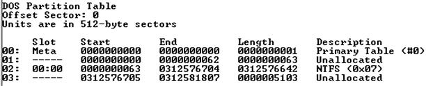
From the sample output that appears in Figure 7.1, we can see the partition table and that the NTFS partition that we would be interested in is the one marked 02, which starts at sector 63 within the image. If you downloaded the “hacking case” image from the NIST site mentioned earlier in this chapter, the output of the mmls command run against the image would look very similar to what is illustrated in Figure 7.1. However, if you get an error that begins with “Invalid sector address,” the image you’re looking at may not have a partition table (such as when an image is acquired of a logical volume rather than the entire physical disk), and you can proceed directly to the part of this chapter where we discuss the use of fls.exe.
You may also find that the partition table isn’t quite as “clean” and simple with some acquired images. Figure 7.2 illustrates the output of mmls.exe run against a physical image acquired from a laptop purchased from Dell, Inc.
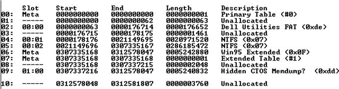
In Figure 7.2, the partition we’d most likely be interested in (at least initially) is the one marked 04, which starts at sector 178176. We will need to have this information (i.e., the sector offset to the partition of interest) available to use with fls.exe (man page found online at http://www.sleuthkit.org/sleuthkit/man/fls.html), in order to extract the file system metadata from within the particular volume in which we’re interested.
Using the offset information, we can collect file system metadata from the partition of interest. Returning to our first example (Figure 7.1, with the NTFS partition at offset 63), the fls.exe command that we would use appears as follows:
In this command, the various switches used all help us get the data that we’re looking for. The “-m” switch allows us to prepend the path with the appropriate drive letter. The “-o” switch allows us to select the appropriate volume. (I’ve included the “-o” switch information in square brackets as it can be optional; if you get an error message that begins with “Invalid sector address” when using mmls.exe, it’s likely that you won’t have to use the “-o” switch at all. Alternately, the value used with the “–o” switch may change, depending on the image you’re using (volume or physical image) or the offset of the volume in which you’re interested. For example, offset 63 would be used for the volume listed in Figure 7.1, but offset 21149696 would be used to extract information from the partition marked 05 in Figure 7.2 (and you’d likely want to use “-m D:/,” as well).) The “-p” switch tells fls.exe to use full paths for the files and directories listed, and the “-r” switch tells fls.exe to recurse through all subdirectories. Explanations for the other switches, as well as additional switches available, can be found on the fls man page at the linked site listed above.
You should also notice that the listed fls command includes a redirection operator, sending the output of the command to a file named “bodyfile.txt.” The bodyfile (described online at http://wiki.sleuthkit.org/index.php?title=Body_file) is an intermediate format used to store the file system metadata information before translating it into the TLN event file format that we discussed earlier.
Using this approach allows us to not just keep track of the information output from our various tools, but to also keep that data available for use with other tools and processes that may be part of our analytic approach. In order to translate the bodyfile (output of the fls.exe command) information to a TLN events file format (the five fields described earlier in this chapter), we want to use the bodyfile.pl script, which is available as part of the additional materials available with this book, in the following command:
The above bodyfile.pl command is pretty simple and straightforward. To see the syntax options available for bodyfile.pl, simply type the command “bodyfile.pl” or “bodyfile.pl –h” at the command prompt. The “-f” switch tells the script which bodyfile to open, and the “-s” switch fills in the name of the server (you can get this from your case documentation, or by running the compname.pl RegRipper plugin against the System hive, as described in Chapter 5). Also, notice that we redirect the output of the command to the events.txt file; as with many of the tools we will discuss, the output of the tool is sent to the console, so we need to redirect it to a file so that we can add to it and parse the events later. Again, the bodyfile.pl script does nothing more than convert the output of the fls command to the necessary format for inclusion in the events file. Once the events file has been populated with all of the events we want to include in our timeline, we will convert the events file to a timeline.
At this point in our timeline creation process, we should have a bodyfile (bodyfile.txt) and an events file (events.txt), both containing file system metadata that was extracted from our acquired image. However, there may be times when we may not have access to an acquired image, or access to the necessary tools, and as such cannot use fls.exe to extract the file system metadata and create the bodyfile. One such example would be accessing a system remotely via F-Response; once you’ve mounted the physical drive on your analysis system, you can then add that drive to FTK Imager as an evidence item just as you would an acquired image. You might do this in order to extract specific files (Registry hives, Event Log files, Prefetch files) from the remote system for analysis. FTK Imager also provides an alternative means for extracting file system metadata, which we can use in situations where we may choose not to use fls.exe.
One of the simplest ways to do this is to open the newly acquired image (or the physical disk for a remote system accessed via F-Response) in FTK Imager, adding it as an evidence item. Figure 7.3 illustrates the image examined in Figure 7.2 loaded into FTK Imager version 3.0.0.1442.
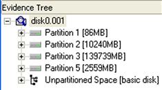
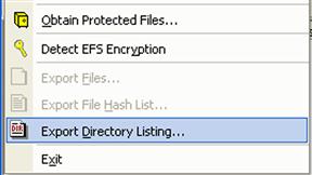
Now, an option available to us once the image is loaded and visible in the Evidence Tree is to select the partition that we’re interested in (say, partition 2 listed in Figure 7.3) and then select the “Export Directory Listing…” option from the File menu, as illustrated in Figure 7.4.
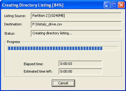
When you select this option, you will then be offered a chance to select the name and location of the comma-separated value (CSV) output file for the command (as part of my case management, I tend to keep these files in the same location as the image itself if I receive the image on writeable media, such as a USB-connected external hard drive). Once you’ve made these selections and started the directory listing process, you will see a dialog such as is illustrated in Figure 7.5.
At this point, we should have a complete directory listing for all of the files visible to FTK Imager in the volume or partition of interest within our image. However, the contents of the file will require some manipulation in order to get the data into a format suitable for our timeline. I wrote the script ftkparse.pl specifically to translate the information collected via this method into the bodyfile format discussed earlier in this chapter. The ftkparse.pl script takes only one argument, which is the path to the appropriate CSV file, and translates the contents of the file to bodyfile format, sending output to the console. An example of how to use the ftkparse.pl script appears as follows:
If you use the above command, be sure to use correct file paths for your situation.
After running the command, if you open the resulting bodyfile in a text editor, you will notice that the file and directory paths appear with some extra information. For example, when I ran through this process on the Vista image described in Figure 7.2, the bodyfile contained paths that looked like “RECOVERY [NTFS]\[root]\Windows\,” where “RECOVERY” is the name of the particular volume from which the directory listing was exported. To get this information into a more usable format, use your text editor (Notepad++works really well for this) to perform a search-and-replace operation, replacing “RECOVERY [NTFS]\[root]\” with “C:\” (or whichever volume or drive letter is appropriate). Once you’ve completed this process with the appropriate volume information, you can then proceed with creating your timeline. The biggest difference between using the FTK Imager directory listing, as opposed to the output of fls.exe, is that the file/directory metadata change date (the “C” in “MACB”) would not be available (FTK Imager does not extract the “C” time) and would be represented as a dot (i.e., “.”) in the bodyfile.
Once you’ve completed this search-and-replace operation, you can run the bodyfile.pl Perl script against the bodyfile.txt file that resulted from running ftkparse.pl, translating it into an events file.
In summary, the commands that you would run to create your events file for file time stamp data from an acquired image using fls.exe would include:
If you opted to use FTK Imager to export a directory listing, the steps you would follow to create an events file for file time-stamped data are:
 Export directory listing via FTK Imager (dir_listing.csv)
ftkparse.pl dir_listing.csv>bodyfile.txt
Search-and-replace file and directory paths with appropriate drive letter
Now, if you’ve created separate events files for different volumes (C:\, D:\, etc.) or even from different systems, you can use the native Windows type command to combine the events files into a single, comprehensive events file, using commands similar to the following:
Notice in the previous command that the redirection operator used is “»,” which allows us to append additional data to a file, rather than creating a new file (or overwriting our existing file by mistake; I’ve done this more than once … a lot more).
Event logs
As discussed in Chapter 4, Event Logs from all versions of Windows can provide a great deal of very valuable information for our timeline; however, how we extract timeline information and create events files for inclusion in our timeline depends heavily on the version of Windows that we’re working with. As we saw in Chapter 4, Event Logs on Windows 2000, XP, and 2003 are very different from the Windows Event Logs available on Vista, Windows 2008, and Windows 7 systems. As such, we will address each of these separately; but ultimately, we will end up with information that we can add to an events file.
Windows XP
Event Log files are found, by default, on Windows 2000, XP, and 2003 systems in the C:\Windows\system32\config directory, and have a.evt file extension. You can normally expect to find the Application (appevent.evt), System (sysevent.evt), and Security (secevent.evt) Event Log files in this directory, but you may also find other files with .evt extensions based on the applications that you have installed. For example, if you have MS Office 2007 (or above) installed, you should expect to find ODiag.evt and OSession.evt files. You can access these files in an acquired image by either adding the image to FTK Imager as an evidence item, navigating to the appropriate directory, and extracting the files, or by mounting the image as a volume via FTK Imager version 3 (or via ImDisk) and navigating to the appropriate directory. Once you have access to these files, you should use the evtparse.pl Perl script to extract the necessary event information using the following command:
This command tells the evtparse.pl script to go to a specific directory, extract all event records from every file in that directory with a.evt extension, and put that information into the evt_events.txt file in TLN format, adding “EVT” as the data source. So, if you’ve mounted an acquired image as the G:\ volume, the argument for the “-d” switch might look like “G:\Windows\system32\config.” Many times, I will extract the Event Log files from the drive or the image using FTK Imager, placing them in a “files” directory, so the path information might then look like “F:\<case>\files.”
If you do not want to run this script against all of the .evt files in a directory, you can select specific files using the “-e” switch. For example, if you want to create an events file using only the event records in the Application Event Log, you might use a command similar to what follows:
I actually use this technique quite often. As I mentioned earlier in this chapter, there are times when I do not want to create a full timeline, but would rather create a mini- or micro-timeline, based on specific data, so that I can get a clear view of specific data without having to sift through an ocean of irrelevant events. For example, I once worked an examination where the customer knew that they were suffering from an infection from specific malware, and informed me that they had installed the Symantec AntiVirus product. After running the evtrpt.pl Perl script (described in Chapter 4) against the Application Event Log, I noticed that there were, in fact, Symantec AntiVirus events listed in the event log (according to information available on the Symantec web site, events with ID 51 indicate a malware detection; evtrpt.pl indicated that there were 82 such events). As such, I used the following command to parse just the specific events of interest out of the Application Event Log:
The resulting events file provided me with the ability to create a timeline of just the detection events generated by the Symantec product, so that I could quickly address the customer’s questions about the malware without having to sift through hundreds or thousands of other irrelevant events.
You’ll notice that unlike the bodyfile.pl script, the evtparse.pl script doesn’t require that you add a server (or user) name to the command line; this is due to the fact that this information is already provided within the event records themselves.
Windows 7
The Windows Event Logs on Vista, Windows 2008, Windows 7 and 8 systems are located (by default) in the C:\Windows\system32\winevt\logs directory and end in the “.evtx” file extension. As discussed in Chapter 4, these files are of a different binary format from their counterparts found on Windows XP and 2003 systems, and as such, we will need to use a different method to parse them and create our events file. Another difference is the names; for example, the primary files of interest are System.evtx, Security.evtx, and Application.evtx. As with Windows XP, additional files may be present depending on the system in question; for example, I have also found the file “Cisco AnyConnect VPN Client.evtx” on a Windows 7 system that had the Cisco client application installed. However, once you get to Vista systems, there are many more Event Log files available; on the system on which I’m currently writing this chapter, I opened a command prompt, changed to the logs directory, and typed “dir”—the result was that a total of 142 files flew by! This does not mean that all of these files are populated with event records; not all of them are actually used by the system. In fact, as you’re conducting your analysis, you’ll find that there are some Windows Event Logs that are populated on some systems and not on others; on my Windows 7 laptop, the Windows Event Logs that include records for remote connections to Terminal Services are not populated because I don’t have Terminal Services enabled; however, on a Windows 2008 R2 system with Terminal Services enabled, I have found those logs to be well populated and extremely valuable. On a side note, I typed the same dir command, this time filtering the output through the find command in order to look for only those Windows Event Logs that included “Terminal” in their name, and the result was nine files. Again, not all of these log files is populated or even used, but they’re there.
As you would expect, parsing these files into the necessary format is a bit different than with Event Log (.evt) files. One method would be to use Andreas Schuster’s Perl-based framework for parsing these files; the framework is available via his blog (found online at http://computer.forensikblog.de/en). Using this framework, you can parse the .evtx files and then write the necessary tool or utility to translate that information to the TLN format. Willi Ballenthin developed his own Python-based solution for parsing .evtx files, which can be found online at http://www.williballenthin.com/evtx/index.html. He also wrote a tool for parsing .evtx records from unstructured or unallocated space called EVTXtract, which can be found online at https://github.com/williballenthin/EVTXtract.
The method that I’ve found to be very useful is to install Microsoft’s Log Parser tool on a Windows 7 system, and then either extract the .evtx files I’m interested in to a specific directory, or mount the image as a volume on my analysis system. From there, I can then run the following command against an extracted System Event Log using the following command:
Logparser -i:evt -o:csv "SELECT RecordNumber,TO_UTCTIME(TimeGenerated),EventID,SourceName,ComputerName,SID,Strings FROM D:\Case\File\System.evtx">system.csv
This command uses the Log Parser tool to access the necessary Windows API to parse the event records from the System.evtx file. The “-i:evt” argument tells Log Parser to use the Windows Event Log API, and the “-o:csv” argument tells the tool to format the output in CSV format. Everything between the “SELECT” and “FROM” tells LogParser which elements of each event record to retrieve and display. Not only can you open this output file in Excel, but you can use the evtxparse.pl Perl script to parse out the necessary event data into TLN format, using the following command:
Again, this process requires an extra, intermediate step when compared to parsing Event Logs from Windows XP systems, but we get to the same place, and we have the parsed data available to use for further analysis. One difference from evtparse.pl is that evtxparse.pl adds the source “EVTX” to the TLN-format events instead of “EVT”; another difference is that the evtxparse.pl script only takes one argument (the file to parse), where evtparse.pl has a number of switches available.
As with the other timeline events files that we’ve discussed thus far, you will ultimately want to consolidate all of the available events into a single events file prior to parsing it into a timeline. You can use a batch file to automate a great deal of this work for you. For example, let’s say that you have an image of a Vista system available on an external hard drive, and the path to the image file is F:\vista\disk0.001. You can mount the image as a volume on your Windows 7 analysis system (i.e., G:\) and create a batch file that contains commands similar to the following to parse the System Event Log (repeat the command as necessary for other Windows Event Log files):
Logparser -i:evt -o:csv "SELECT RecordNumber,TO_UTCTIME(TimeGenerated),EventID,SourceName,ComputerName,SID,Strings FROM %1\Windows\system32\winevt\logs\System.evtx">%2\system.csv
If you name this batch file “parseevtx.bat,” you would launch the batch file by passing the appropriate arguments, such as follows:
Running the previous command populates the %1 variable in the batch file with your first command line parameter (in this case “G:,” representing your mounted volume) and the %2 variable with your second command line parameter (in this case “F:\vista,” representing the path to where your output should be stored), and executes the command. You would then use (and repeat as necessary) a command similar to the following to parse the output .csv files into event files:
Again, you will need to repeat the above command in the appropriate manner for each of the Windows Event Logs parsed. Another available option, if you want to parse several Windows Event Log files in succession, is to use the “*” wildcard with the Logparser command, as follows:
Logparser -i:evt -o:csv "SELECT RecordNumber,TO_UTCTIME(TimeGenerated),EventID,SourceName,ComputerName,SID,Strings FROM %1\Windows\system32\winevt\logs\* evtx">%2\system.csv
This command will parse through all of the .evtx files in the given folder (entered into the batch file as the first argument, or %1). With all of these different records, there are going to be a wide range of SourceName and EventID values to deal with, and it’s likely going to be impossible to memorize all of them, let alone just the ones of interest. In order to make this a bit easier, I added something to the evtxparse.pl Perl script—actually, I embedded it. One of the first things that the script (or executable, if you’re using the “compiled” version of the tool) will do is look for a file named “eventmap.txt” in the same directory as the tool. Don’t worry, if the file isn’t there, the tool won’t stop working—but it works better with the file. In short, what this file provides is event mappings, matching event source, and IDs to a short descriptor of the event. For example, if the event source is “Microsoft-Windows-TerminalServices-LocalSessionManager” and the event ID is 21, this information is mapped to “[Session Logon],” which is much easier to understand than “Microsoft-Windows-TerminalServices-LocalSessionManager/21.”
The eventmap.txt file is a simple text file, so feel free to open it in an editor. Any line in the file that starts with “#” is treated as a comment line and is skipped; some of these lines point to references for the various information that I’ve accumulated in the file thus far, so that it can be verified. All of the event mapping lines are very straightforward and easy to understand; in fact, the structure is simple so that you can add your own entries as necessary. I would suggest that if you do intend to add your own mapping lines, just copy the format of the other lines and be sure to include references to that you can remember where you found the information. In this way, this tool becomes self-documenting; once you’ve added any entries and references, they’re in the file until they’re removed, so all you would need to do is copy the eventmap.txt file into your case folder.
Prefetch files
As discussed in Chapter 4, not all Windows systems perform application prefetching by default; in fact, Prefetch files are only usually found on Windows XP, Vista, and Windows 7 and 8 systems (application prefetching is disabled by default on Windows 2003 and 2008 systems, but can be enabled via a Registry modification). Also, Prefetch files can contain some pretty valuable information; for the purpose of this chapter, we’re interested primarily in the time stamp embedded within the file. We can use the pref.pl Perl script to extract the time value for the last time the application was run (which should correspond closely to the last modification time of the Prefetch file itself) and the count of times the application has been run into TLN format, using the following command:
Now, we have a couple of options available to us with regard to the previous command. For example, as the command is listed, the “-d” switch tells the tool to parse through all of the files ending with the “.pf” (the restriction to files ending in “.pf” is included in the code itself) extension in the Prefetch directory (of an acquired image mounted as the G:\ volume); if you would prefer to parse the information from a single Prefetch file, simply use the “-f” switch along with the full path and filename for the file of interest. By default, the pref.pl script will detect which version of Windows from which the Prefetch files originated and automatically seek out the correct offsets for the metadata embedded within the file. The “-t” switch tells the Perl script to structure the output in TLN format and adds “PREF” as the source. Also, you’ll notice that as with some other scripts that we’ve discussed thus far, pref.pl has a “-s” switch with which you can add the server name to the TLN format; Prefetch files are not directly associated with a particular user on the system, so the user name field is left blank.
Finally, at the end of the command, we redirected the output of the script to the file named “pref_events.txt.” Instead of taking this approach, we could have easily added the output to an existing events file using “» events.txt.”
Registry data
As we’ve discussed several times throughout this book, the Windows Registry can hold a great deal of information that can be extremely valuable to an analyst. Further, that information may not solely be available as Registry key LastWrite times. There are a number of Registry values that contain time stamps, available as binary data at specific offsets depending on the value, as strings that we need to parse, etc. As such, it may be useful to have a number of different tools available to us to extract this information and include it in our timelines.
Perhaps one of the easiest ways to incorporate Registry key LastWrite time listings within a timeline is to use the regtime.pl Perl script (part of the additional materials available for this book). I was originally asked some time ago to create regtime.pl in order to parse through a Registry hive file and list all of the keys and their LastWrite times in bodyfile format; that is, to have the script output the data in a format similar what fls.exe produces. I wrote this script and provided it to Rob, and it has been included in the SANS Investigative Forensic Toolkit (SIFT) workstation (found online at http://computer-forensics.sans.org/community/downloads/), as well as Kristinn’s log2timeline framework. A bit ago, I modified this script to bypass the bodyfile format and output its information directly to TLN format. An example of how to use this updated version of regtime.pl appears as follows:
Similar to the fls.exe tool discussed earlier in this chapter, regtime.pl includes a “-m” switch to indicate the “mount point” of the Registry hive being parsed, which is prepended to the key path. In the above example, I used “HKEY_USER” when accessing a user’s Registry hive; had the target been a Software or System hive, I would have need to use “HKLM/Software” or “HKLM/System,” respectively. The “-r” switch allows you to specify the path to the hive of interest (again, either extracted from an acquired image or accessible by mounting the image as a volume on your analysis system). As you would expect, the “-s” and “-u” switches allow you to designate the system and user fields within the TLN format, as appropriate; the script will automatically populate the source field with the “REG” identifier.
With respect to parsing time-stamped information from within Registry values, there are two options that I like to use: one involves RegRipper, described in Chapter 5. By making slight modifications to rip.pl (new version number is 20110516) and adding the ability to add a system and user name to the TLN output, I can then also modify existing RegRipper plugins to output their data in TLN format. For example, I modified the userassist.pl RegRipper plugin to modify its output format into the five-field TLN format and renamed the plugin “userassist_tln.pl.” I could then run the plugin using the following command line:
An excerpt of the output of this command appears as follows in TLN format:
1163016851|REG|SERVER|USER|UserAssist - UEME_RUNCPL:SYSDM.CPL (4)
1163015716|REG|SERVER|USER|UserAssist - UEME_RUNCPL:NCPA.CPL (3)
1163015694|REG|SERVER|USER|UserAssist - UEME_RUNPATH:C:\Putty\putty.exe (1)
Clearly we’d want to redirect this output to the appropriate events file (i.e., “» events.txt”) for inclusion in our timeline.
There are a number of RegRipper plugins that provide timeline-format output, many of which can provide valuable insight and granularity to your timeline. It’s very easy to determine which plugins provide this information by typing the following command:
What this command does is list all of the available RegRipper plugins in .csv format, so that each entry is on a single line, and it then runs the output through the find command, looking for any plugins that include “_tln” in the name. The output of the above command will appear in the console, so feel free to redirect the output to a file for keeping and review. If you send the output to a .csv file, you can open it in Excel and sort on the hive to which the plugin applies (System, Software, NTUSER.DAT, USRCLASS.DAT, etc.), making it easier to pick which ones may be applicable to your analysis and you’d like to run.
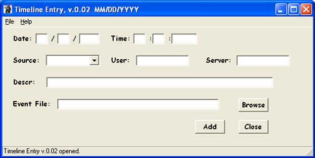
Another means for adding any time-stamped information (other than just from the Registry) to a timeline events file is to use the graphical user interface (GUI) tln.pl Perl script, as illustrated in Figure 7.6.
Okay, how would you use the GUI? Let’s say that rather than running the userassist_tln.pl plugin mentioned above, we instead ran the userassist2.pl plugin against the same hive file, and based on the nature of our investigation we were only in the entry that appears as follows:
Opening the tln.pl GUI, we can then manually enter the appropriate information into the interface, as illustrated in Figure 7.7.
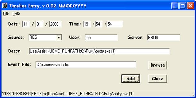
Once you’ve added the information in the appropriate format (notice that the date format is “MM/DD/YYYY,” and a reminder even appears in the window title bar; entering the first two values out of order will result in the date information being processed incorrectly) and hit the “Add” button, the information added to the designated events file appears in the status bar at the bottom of the GUI.
I wrote this tool because I found that during several examinations, I wanted to add specific events from various sources to the events file, but didn’t want to add all of the data available from the source (i.e., Registry), as doing so would simply make the resulting timeline larger and a bit more cumbersome to go through when conducting analysis. For example, rather than automatically adding all UserAssist entries from one or even from several users, I found that while viewing the output of the userassist2.pl RegRipper plugin for a specific user, there were one or two or even just half a dozen entries that I felt were pertinent to the examination and added considerable context to my analysis. I’ve also found that including the creation date from the MFT $FILE_NAME attribute for one or two specific files, depending on the goals of my exam, proved to be much more useful than simply dumping all of the available MFT data into the timeline.
Additional sources
To this point in the chapter, we’ve discussed a number of the available time-stamped data sources that can be found on Windows systems. However, I need to caution you that these are not the only sources that are available; they are simply some of the most common ones used to compile timelines. In fact, the list of possible sources can be quite extensive (a table listing source identifiers, descriptions, and tools used to extract time-stamped data is included in the materials associated with this book); for example, Windows shortcut (.lnk) files contain the file system time stamps of their target files embedded within their structure. Earlier we mentioned that the Firefox bookmarks.html file might contain useful information, and the same thing applies to other browsers, as well as other applications. For example, Skype logs might prove to be a valuable source of information, particularly if there are indications that a user (via the UserAssist subkey data) launched Skype prior to or during the time frame of interest.
Speaking of UserAssist data from user Registry hive files, another data source worth mentioning is VSCs. As illustrated and discussed in Chapter 3, a great deal of time-stamped data can be retrieved from previous copies of files maintained by the Volume Shadow Copy Service (VSS), particularly on Vista and Windows 7 systems. One of the examples we saw in Chapter 3 involved retrieving UserAssist data from the hive file within a user’s profile. Consider an examination where you found that the user ran an image viewer application, and that application maintains an MRU list of accessed files. We know that the copy of the user’s NTUSER.DAT hive file would contain information in the UserAssist key regarding how many times that viewer application was launched, as well as the last date that it was launched. We also know that the MRU list for the viewer application would indicate the date and time that the most recently viewed image was opened in the application. As we saw in Chapter 3, data available in previous versions of the user’s NTUSER.DAT hive file would provide not just indications of previous dates that the viewer application was run, but also the dates and times that other images were viewed. Depending upon the goals of your examination, it may be a valuable exercise to mount available VSCs and extract data for inclusion in your timeline.
So, this chapter should not be considered an exhaustive list of data sources, but should instead illustrate how to easily extract the necessary time-stamped data from a number of perhaps the most critical sources. Once you have that data, all that remains is to convert it into a normalized format for inclusion in your timeline.
Parsing events into a timeline
Once we’ve created our events file, we’re ready to sort through and parse those events into a timeline, which we can then use to further our analysis. So, at this point, we’ve accessed some of the various data sources available on a Windows system and created a text-based, pipe-delimited, TLN-format events file. The contents of this file might appear as follows:
1087549224|FILE|SERVER||MACB [0] C:/$Volume
1087578198|FILE|SERVER||MACB [0] C:/AUTOEXEC.BAT
1087578213|FILE|SERVER||..C. [194] C:/boot.ini
1087576049|FILE|SERVER||MA.. [194] C:/boot.ini
1087549489|FILE|SERVER||...B [194] C:/boot.ini
1087578198|FILE|SERVER||MACB [0] C:/CONFIG.SYS
1200617554|FILE|SERVER||.A.. [56] C:/Documents and Settings
1087586327|FILE|SERVER||M.C. [56] C:/Documents and Settings
1200617616|EVT|SERVER|S-1-5-18|Service Control Manager/7035;Info;IMAPI CD-Burning COM Service,start
1200617616|EVT|SERVER|N/A|Service Control Manager/7036;Info;IMAPI CD-Burning COM Service,running
1200617616|EVT|SERVER|N/A|Service Control Manager/7036;Info;IMAPI CD-Burning COM Service,stopped
1200617621|EVT|SERVER|N/A|EventLog/6006;Info;
1087585113|PREF|SERVER||AGENTSVR.EXE-002E45AB.pf last run (1)
We should be ready to parse the events file into a timeline, the purpose of which is to sort through the events within the events file, grouping those that occur within the same time together, and then sorting them and presenting them in an understandable format. I’ve written a script for this purpose, aptly named parse.pl, and the simplest, most basic way to use this script is to run it against your events file using a command line similar to the following:
This command produces an ASCII-based timeline file with all of the times sorted with the most recent time first, and with all events within the same time grouped together. The output looks like:
An example of what this might look like in a “real” timeline file appears as follows:
FILE SERVER - MACB [12864] C:/WINDOWS/Prefetch/DFRGNTFS.EXE-269967DF.pf
FILE SERVER - MACB [8622] C:/WINDOWS/Prefetch/DEFRAG.EXE-273F131E.pf
FILE SERVER -.A.. [99328] C:/WINDOWS/system32/dfrgntfs.exe
It should be easy to see from this timeline format how the five-field TLN format plays right into not just collecting and correlating the events, but also displaying them for analysis. Again, the times are formatted in a human-readable format, based on UTC. Normalizing the times to this format allows us to incorporate data from multiple sources independent of time zone or location and present the information in a uniform manner. All of the events that occurred within that second are then listed below the time value, slightly indented. This text-based format allows you to browse through the timeline using any text editor (as opposed to requiring a specific editor or viewer). I use UltraEdit, as it’s very good at handling large files, and if I find some text of interest that I want to search on, I can highlight the text and hit the F3 key to automatically jump to the next instance of that text.
The parse.pl Perl script also provides some additional capabilities that can be very useful to you. For example, if you know that you’re looking for all events that occurred within a particular time window, you can use the “-r” switch to specify a time window for the events that will be displayed within the timeline. For example:
The above command line will parse the events file, but only place events that occurred between 00:00:00 February 12, 2008, and 23:59:59 March 16, 2008, into the timeline file.
Another option that I recently added to parse.pl is the ability to output the timeline information to CSV or .csv format, which would allow you to open the output file in a spreadsheet application such as MS Office Excel or OpenOffice Calc. When the information is written to the timeline file, all five fields are included on each line, separated by commas, so each row in the spreadsheet application begins with a time value in the “YYYYMMDDhhmmss” format. Spreadsheets have long been used to view and analyze this sort of time-stamped information, although in the past the information was populated manually. One of the aspects of this approach that I really think is useful to a lot of analysts is that the analyst can highlight specific events with color coding and can even add notes into a sixth column (e.g., adding MS KnowledgeBase articles as references, notes to clarify the information that is available in the timeline).
The parse.pl script has two additional capabilities. First, the “-o” switch will list the timeline with the oldest events; by default, the most recent events will appear first. Second, by default, the script will automatically remove duplicate entries; this comes in handy when you’ve added data from VSCs and not all of it has changed. You may parse some data sources from within a VSC, such as the UserAssist information for a user (as discussed previously in this chapter), and some entries have the exact same values in all five fields of the TLN output. You likely don’t want this duplicate data populating your timeline, so the parse.pl script will automatically remove these duplicate entries.
So now that we have a timeline, how do we go about analyzing it? I think that the best way to do this is with an example. An excerpt from a timeline created from a system that had experienced a malware infection (trimmed to make it easier to view and with slight modifications) appears as follows (times removed to make the information easier to view):
FILE SYSTEM -...B [720] C:/WINDOWS/system32/irrngife.dat
FILE SYSTEM -...B [506] C:/WINDOWS/system32/msgsvuc.dat
FILE SYSTEM -...B [2700] C:/WINDOWS/system32/kbdrxyl.dat
FILE SYSTEM -...B [0] C:/Documents and Settings/user/Local Settings/Temp/~~x103D.tmp
REG SYSTEM - - M... HKLM/Software/Classes/CLSID/{GUID}
REG SYSTEM - - M... HKLM/Software/Classes/CLSID/{GUID}/InprocServer32
REG SYSTEM - - M... HKLM/Software/Microsoft/Windows/…/ShellIconOverlayIdentifiers/msgsvuc
Other portions of the timeline appeared similar to what you see above, with specific Registry keys being created and grouped along with specific .dat files being created (remember, “B” refers to the “born” date) within the system32 directory. By looking for groupings similar to this throughout the timeline, you can distinguish between infections and other events where the installed AV product detected a malicious file and deleted it before any further actions could occur.
Thoughts on visualization
I’ve talked to a number of analysts and read questions posted to online forums regarding the use of visualization tools and techniques with timeline analysis. Most of these questions seem to center around entering all of the available event data into some sort of visualization model or tool, so that the analyst can then perform analysis. This isn’t something that, at this point, I can see being entirely feasible or useful toward furthering analysis.
Yes, I know that having some sort of visualization tool seems as if it would make things much easier for the analyst, but we have to keep in mind that Windows systems are extremely verbose, even when they’re just sitting there, apparently idle. By themselves, Windows systems will perform housekeeping functions, creating and deleting System Restore Points and VSCs, installing updates, performing limited defrags of the hard drive, etc. Once you include some of the applications and their automated functions (Java and Apple products, among others, automatically look for updates), it becomes clear that there’s a lot that goes on on Windows systems when no one’s around. So if you think back to Chapter 1 where we discussed Least Frequency of Occurrence, it quickly becomes clear that any sort of visualization mechanism for representing the abundance of time-stamped data available on a Windows system will quickly not simply overwhelm the analyst, but also completely mask the critical events of interest.
What this really comes down to is how an analyst uses timelines for analysis; even so, once analysis has been performed, the analyst’s job isn’t complete—her findings still need to be reported and presented to the “customer.” Most often pertinent excerpts of timelines are included in the report as a narrative or encapsulated in a table, although there are templates for spreadsheet applications that will allow you to create visual timelines; these should only be used after the pertinent events have been clearly identified; otherwise, everyone (the analyst, the customer, etc.) will be overwhelmed by the sheer volume of available data.
Case Study
After all of this discussion, it would be a good idea to do a complete walk-through of the process for creating a timeline from an acquired image. As such, this will require an image to use and a great place to go online to get one is Lance Mueller’s first forensic practical posted via his blog (found online at http://www.forensickb.com/2008/01/forensic-practical.html). The first thing you will need to do is to download the 400-MB expert witness format (EWF, also known as “Encase” format) image, and then open it in FTK Imager (get version 3 from the AccessData downloads page if you don’t already have it) and reacquire the image into a 1.5-GB raw/dd format image file named “xpimg.001.” We’ll be using this name throughout the rest of this case study; if you use a different name, use that name. Also, from the scenario that Lance provided on his web site, this appears to be a malware-related issue, so this would likely be a good opportunity to develop a timeline.
Once you have the raw/dd format image available, you’ll see when you run the mmls command described earlier in this chapter that you get the “Invalid sector address” error message, which is an indication that a partition table wasn’t found. As such, you can proceed directly to using the fls command without the need for an offset to a specific partition. You can use the following command to create the bodyfile from the file system metadata within the image:
We can then use FTK Imager version 3 to mount the image on our analysis system (as the F:\ volume) and use rip.pl to obtain the system name, using the following command:
From this command, you will see that the system name is “REG-OIPK81M2WC8.” You can then use the following command to parse the bodyfile into the events file:
At this point, you’ve created your initial events file, and you can then go about adding Event Logs records and Prefetch file metadata as additional data sources using the following commands:
C:\tools>evtparse.pl -d f:\[root]\Windows\system32\config -t » D:\case\events.txt
C:\tools>pref.pl -d f:\[root]\Windows\Prefetch -s REG-OIPK81M2WC8 -t » D:\case\events.txt
As part of your process for detecting malware, you run RegRipper against various hive files available within the image, including the NTUSER.DAT hive for the “vmware” user. When examining the RegRipper output file from this hive for malware autostart locations (something you remembered from Chapter 6), you notice an unusual value in the CurrentVersion\Run key and enter that single entry into your events file using tln.pl, as illustrated in Figure 7.8.
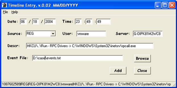
Based on this, you then decided to add the UserAssist subkey information for that user to your events file using the following command:
C:\tools>rip.pl -r "f:\[root]\Documents and Settings\vmware\ntuser.dat" -u vmware -s REG-OIPK81M2WC8 -p userassist_tln » D:\case\events.txt
You then run regtime.pl against the System and Software hives from within the image in order to add the time-stamped data from these Registry hives to your events file using the following commands:
C:\tools>regtime.pl -r f:\[root]\Windows\system32\config\software -m HKLM/Software -s REG-OIPK81M2WC8 » D:\case\events.txt
C:\tools>regtime.pl -r f:\[root]\Windows\system32\config\system -m HKLM/System -s REG-OIPK81M2WC8 » D:\case\events.txt
At this point, you have a pretty comprehensive events file compiled, and you decide to parse it into a timeline. Using this technique, you can take an iterative approach, by adding additional events as necessary to the events file and regenerating the timeline file, as necessary. To create your timeline file, you can use the following command:
You then open your newly created timeline file in a text editor and search for inetsrv\rpcall.exe within the timeline and find the following entries:
FILE REG-OIPK81M2WC8 -..C. [524288] C:/Documents and Settings/vmware/NTUSER.DAT
FILE REG-OIPK81M2WC8 - MACB [21396] C:/WINDOWS/Prefetch/SMS.EXE-01DC4541.pf
FILE REG-OIPK81M2WC8 -...B [15870] C:/WINDOWS/Prefetch/RPCALL.EXE-394030D7.pf
FILE REG-OIPK81M2WC8 - M.C. [152] C:/WINDOWS/system32/inetsrv
FILE REG-OIPK81M2WC8 -.A.. [16384] C:/WINDOWS/system32/ping.exe
PREF REG-OIPK81M2WC8 - PING.EXE-31216D26.pf last run (1)
PREF REG-OIPK81M2WC8 - RPCALL.EXE-394030D7.pf last run (2)
PREF REG-OIPK81M2WC8 - SMS.EXE-01DC4541.pf last run (2)
REG REG-OIPK81M2WC8 vmware - UserAssist - UEME_RUNPATH:C:\System Volume Information\...\RP2\snapshot\Repository\FS\sms.exe (1)
REG REG-OIPK81M2WC8 vmware - HKCU\..\Run - RPC Drivers ->C:\WINDOWS\System32\inetsrv\rpcall.exe
REG REG-OIPK81M2WC8 - M... HKLM/Software/Microsoft/Windows/CurrentVersion/Run
REG REG-OIPK81M2WC8 - M... HKLM/Software/Microsoft/Windows/CurrentVersion/RunServices
REG REG-OIPK81M2WC8 - M... HKLM/System/ControlSet001/Services/SharedAccess/Parameters
REG REG-OIPK81M2WC8 - M... HKLM/System/ControlSet001/Services/SharedAccess/Parameters/FirewallPolicy
REG REG-OIPK81M2WC8 - M... HKLM/System/ControlSet001/Services/SharedAccess/Parameters/FirewallPolicy/StandardProfile
REG REG-OIPK81M2WC8 - M... HKLM/System/ControlSet001/Services/SharedAccess/Parameters/FirewallPolicy/StandardProfile/AuthorizedApplications
REG REG- OIPK81M2WC8 - M... HKLM/System/ControlSet001/Services/SharedAccess/Parameters/FirewallPolicy/StandardProfile/AuthorizedApplications/List
Noticing the entries at the end of the listing that point to the firewall settings on the system (from the System hive), you then run RegRipper against the System hive and looking at the firewall settings output for the report file, find the following:
C:\WINDOWS\System32\inetsrv\rpcall.exe ->C:\WINDOWS\System32\inetsrv\rpcall.exe::Enabled:RPC Drivers
So at this point in your analysis, you have likely found a good candidate for the malware thought to be on the system; in this case, the rpcall.exe file. Not only that, you have additional context available regarding how the malware was activated on the system; specifically, from the above timeline listing, you see the following:
vmware - UserAssist - UEME_RUNPATH:C:\System Volume Information\...\RP2\snapshot\Repository\FS\sms.exe (1)
This indicates that sms.exe was run from the “vmware” user context, but the path indicates that the executable file itself was found within a System Restore Point (RP2). You know that users should not normally be able to access this directory path, let alone launch executable files. An additional search of the timeline indicates that the tool cacls.exe, which can be used to modify permissions of various objects (files, directories, Registry keys) on Windows systems, was run shortly before the timeline listing we see above.
While this is a brief case study, my hope is that it serves to demonstrate how powerful and beneficial timeline analysis can be, and that it encourages analysts to explore the use of this as viable analysis technique. Not only does it demonstrate how timelines can be used to detect the presence of malware within an image (often much faster than or even in lieu of AV), but it also illustrates the concept of context that we discussed earlier in this chapter, as well as how timelines can provide an increased level of relative confidence with respect to the various data sources used to populate the timeline. Finally, while the original image file was 1.5 GB in size, the resulting timeline file is just under 6 MB and compresses down to 511 KB.
Summary
Properly employed, timelines can be an extremely valuable analysis tool. The nature of our complex operating systems, applications, and various other data sources almost necessitates an open-source approach to creating tools for parsing time-stamped data and converting it into a normalized format. Timelines can provide and facilitate a level of visibility into examinations that analysts have not seen using commercial forensic analysis applications, in cases ranging from malware infections, to suspected intrusions, to violations of acceptable use policies and contraband image cases, as well as the more “advanced” incidents that have been discussed in the media.
The open-source approach also means that an analyst isn’t restricted to a specific analysis platform; many of the available tools and scripts, including those discussed in this chapter, can be run on Linux and MacOS X platforms, often without any modification.
However, analysts should keep in mind that as versatile and powerful a technique as this is, it’s still just a tool and isn’t necessarily something that would or should be employed in every situation. Be sure that you fully understand the goals of your analysis before you decide to employ any particular tool, including timeline analysis.
Finally, in this chapter, we’ve discussed a number of tools that can be used for creating timelines. These tools simply make up and implement the approach that I’ve used to create timelines, and this chapter has been about the process of creating a timeline, not about tools themselves. That being said, all of the tools discussed are command line tools, and I’m aware that there are a good number of analysts who aren’t entirely familiar with how to use or run command line tools; that’s okay. Most of the tools we’ve discussed are Perl scripts, and the source code for these tools is provided online with the materials for this book. If at any point you have questions about what the tool is capable of doing, or what options are available within the tool, you can open the Perl scripts in an editor (Notepad++is a great option). Another option is that for your convenience, I’ve provided standalone Windows executables for each tool (“compiled” using Perl2Exe), and you can type the command by itself, or followed by “-h” or “/?,” to see what options are available.