LECTURE 15

Proof of the Existence of Walrasian Equilibrium

1. Case of a Single Labor Sector

In the previous lecture we derived a set of conditions necessarily satisfied at any price equilibrium. In the present lecture, we shall show that these conditions are also sufficient, and that they may all be satisfied simultaneously. In this way we shall establish the existence of a price equilibrium for the model introduced in Lecture 13, i.e., we shall show the existence of prices p_j such that the following conditions are satisfied

(a) P_j ≥ 0, j = 0, . . ., N; moreover, for some k, p_k > 0

(b) max subject to

(See Lecture 13 for a more precise statement.)

(c) = max subject to

(See Lecture 13 for a more precise statement.)

We recall that these conditions have the following briefly stated heuristic significance:

(a) the price of each commodity is nonnegative;

(b) each firm operates so as to maximize its profits subject to its capital limitations;

(c) each consumption unit optimizes its own utility function subject to its own budgetary constraints, and

(d) whatever is consumed must be produced, and overproduction cannot occur for a commodity whose price is positive.

Having established the existence of a set of prices, production schemes, and consumption schemes satisfying (a)–(d) above, we shall formulate a more general model, in which not one but several kinds of labor will be included, and show the existence of a general price equilibrium in that case also.

2.A Preliminary Existence Theorem

We shall proceed by setting up an ansatz giving prices, production, consumption, etc., as functions of a rate-of-profit parameter ρ, and then choosing ρ so as to obtain a price equilibrium. In determining the form of our ansatz, we will of course be guided by the analysis carried out in the preceding lecture. Let us begin by assuming prices p_j(ρ) as solutions of the equation

where ρ is a parameter; we know from Lecture 3 that a nonnegative (and nontrivial) solution of these equations exists for all values of ρ satisfying 0 ≤ ρ ≤ ρ_max and that these prices satisfy condition (a), provided only that is a connected matrix. The matrix will be assumed to be connected throughout the present lecture. Note that this implies that the prices P_j(ρ),j = 1, . . ., n, are strictly positive for all ρ, 0 ≤ ρ ≤ ρ_max. The price p₀(ρ) is positive if and only if ρ ≠ ρ_max, While P₀(ρ_max) = 0.

Next we choose the consumption levels S_j^(v) so as to maximize each of the utility functions u^(v) subject to the constraint

where, as in the preceding lecture, we put

As we saw in the preceding lecture, this condition determines the quantities s_j^(v) as functions of the rate of profit ρ. We define the total consumption s_i(ρ) of the ith commodity as

Finally, we determine the total production of the ith commodity by the equation

We put for convenience.

The following lemma then reduces the problem of establishing the existence of a price equilibrium to a more tractable form.

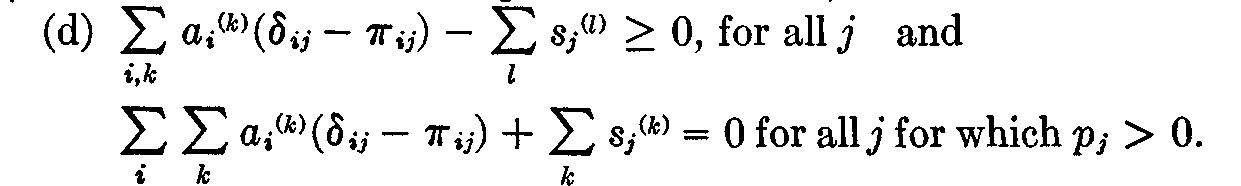
LEMMA 15.1. Let the prices, consumption, and total production be determined from ρ as above. Then there will exist a determination of the production levels a_j^(k) for the various firms satisfying

which, together with the prices and consumption schemes determined above, will satisfy the conditions (a)–(d), i.e., will define a price equilibrium, provided that

and provided also that

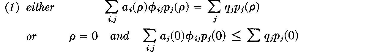
Proof: If the prices satisfy (15.1), they are nonnegative and not all zero so that (a) is satisfied. If in condition (1) we have ρ > 0, it is plain that we may divide the total production levels a_j(ρ) into individual-firm contributions a_j^(k) as in (15.5), in such a way that

for each k, k = 1, . . ., m. Similarly, if in condition (1) we have ρ = 0, we may divide the total levels into individual-firm contributions in such a way that

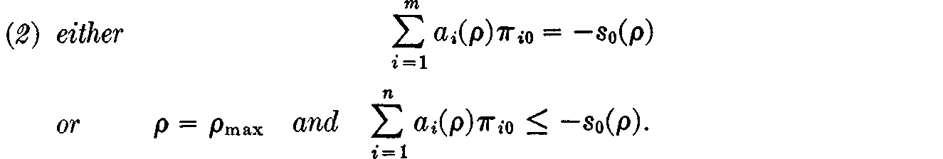
for each k, k = 1, . . ., m. Thus, if condition (1) is satisfied, we may in any case divide the total production levels a_j(ρ) into individual-firm contributions in such a way that no firm’s production plans will require the outlay of more capital than it possesses; moreover, unless ρ = 0, each firm will make use of the whole of its capital. As we have seen in the previous lecture, this, coupled with (15.1), is just the condition that each firm’s profits be maximized. Thus (b) of our conditions, defining a price equilibrium, is satisfied. We have determined the consumption schemes in such a way that (c) is automatically satisfied. Finally, since all the relations in (d) except the first, i.e., the j = 0 relations, are satisfied in consequence of the way the have been defined, and since condition (2) is the condition that the j = 0 relation be satisfied also (recall that ρ = ρ_max means that the price of labor is zero), condition (d) is also satisfied. Q.E.D.

In the trivial case ρ_max = 0, we have p₀ = 0 and ρ = 0, so that = 0 for j ≥ 1 by (15.2) and (15.3); thus s_j = 0 for j ≥ 1 by (15.4) and a_j = 0 by (15.5), so that the above lemma tells us that a price equilibrium exists and is to be determined by our formulas (15.1)–(15.5). We consequently may, and shall unless the contrary is explicitly indicated, assume in what follows that ρ_max > 0.

Let us define the demand for labor d₀(ρ) by

and recall that we have already defined the supply of labor –s₀(ρ) by (14.5). The following useful identity reduces the conditions of Lemma 1 to a more manageable form.

LEMMA 15.2. Let a_i(ρ), p_i(ρ), s₀(ρ), and d₀(ρ) be as above. Then

Proof: Consider the expression

All terms in this expression, except possibly the j = 0 term, are zero by (15.5). Therefore (15.8) is just

or, equivalently,

But (15.8) can be written (using (15.1), (15.2), and (15.3)) as

Therefore

Q.E.D.

Putting together Lemmas 1 and 2 yields the following corollary:

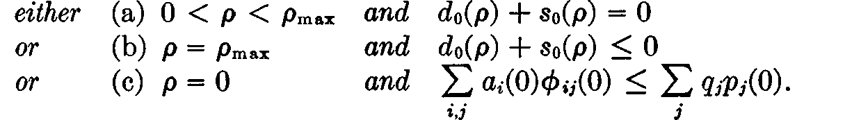
COROLLARY 15.3. Let prices and total production be determined from ρ as above. Then there will exist a determination of the production levels for the various firms satisfying (15.6), which, together with the prices and consumption schemes determined above, will define a price equilibrium, provided that

Lemma 2 also yields trivially the following corollary, which states a fact used in the construction of the diagrams of the previous lecture and also gives an equivalent alternate version of the condition under (c) of the preceding corollary.

COROLLARY 15.4.

Proof: Statement (i) follows from Lemma 2, and statement (ii) follows from statement (i) and Lemma 2. Q.E.D.

We have supposed that ρ_max > 0. Using what we have proved we may distinguish three possibilities for s₀(ρ) + d₀(ρ). The first is that for some ρ, 0 < ρ ≤ ρ_max, supply and demand for labor are equal, i.e., s₀(ρ) + d₀(ρ) = 0. The second is that for all ρ, 0 < ρ ≤ ρ_max, –s₀(ρ) < d₀(ρ). The third possibility is that for all ρ, 0 < ρ ≤ ρ_max, it is the case that –s₀(ρ) > d₀(ρ). Note that in any case, by Corollary 4, s₀(0) + d₀(0) = 0.

In the first case, condition (a) of Corollary 3 is satisfied. In the second case, since s₀(ρ) + d₀(ρ) is positive for ρ > 0 and zero for ρ = 0, the derivative of s₀(ρ) + d₀(ρ) is nonnegative at ρ = 0, so that by Corollary 4, condition (c) of Corollary 3 is satisfied. If S₀(ρ) + d₀(ρ) is negative for ρ > 0, the condition (b) of Corollary 2 is satisfied. This establishes the existence of a price equilibrium in every case.

The following theorem summarizes the necessary conditions for equilibrium derived in the preceding lecture and the sufficient conditions derived in the present section.

THEOREM 15.5. Let ϕ₀(ρ) = s₀(ρ) + d₀(ρ), where s₀(ρ), d₀(ρ) are defined as above. Then price equilibria correspond to those values 0 < ρ < ρ_max for which ϕ₀(ρ) = 0; and also to the value ρ = ρ_max if and only if and also to the value ρ = ρ_max if and only if ϕ₀(ρ_max) ≤ 0. At each such equilibrium the prices are unique; the total activity levels are also unique, and these totals may be divided among the firms in any way consistent with the requirement

3.Price Equilibrium for a Nonhomogeneous Labor Force

We now extend our price-equilibrium model to include several labor sectors, considered as originating labor commodities C₀, C_–1, . . ., C_–L. If ρ_max = 0, no wages can be paid; hence the distinction between labor sectors is entirely irrelevant, and we return to the model of the preceding section. Hence we may and shall assume without loss of generality that ρ_max > 0.

In the present more general context, we shall reestablish results much like those of the two preceding lectures. We will find, in particular, that price equilibria exist whenever supply and demand for labor are simultaneously in balance in all of the labor sectors.

As we have seen in Lecture 3, prices may be determined by the basic relation (15.1) (the range of summation of j being extended from –L to N) as functions of ρ and of the ratios θ_j (j = 0, . . ., L) of the wages, where we normalize these ratios by demanding that Thus, letting p_j(ρ, θ) be the prices so determined, we can write

We shall assume throughout the present section that each form of labor is required as input to the production of at least one commodity, and shall also assume that the n × n matrix obtained by deleting all elements of π_iJ but those with both i and j between 1 and n, is connected.

To construct a price equilibrium, we imitate the procedure of the preceding sections, as follows. The consumption levels s_j^(v) are again chosen so as to maximize

over all s_j such that

This determines total consumption, defined by

Total activity levels are then defined by the equations

and we define the demand for labor in the various sectors by

The above formulae define individual-family consumption schemes, prices, and total production as functions of ρ and θ, but not the division of total production among the individual firms. It will be convenient in what follows to speak of those values of ρ and θ for which the total production levels a_j may be divided into the sum of individual-firm contributions a_j^(k) to yield a set of individual-firm production levels, family consumption and labor schemes, and prices satisfying the conditions (a)–(d) defining a price equilibrium as values ρ, θ corresponding to a price equilibrium. This terminology will be employed in stating a number of the theorems and lemmas which are to follow. Put

We aim to obtain the following result.

THEOREM 15.6. A. A price equilibrium will correspond to each of those and only those points 0 < ρ ≤ ρ_max, θ₀, . . ., θ_L, for which ϕ_–j(ρ, θ) ≤ 0 for all j = 0, . . ., L with equality whenever p_–j(ρ, θ) ≠ 0; and also to those and only those points ρ = 0, θ₁, . . ., θ_n for which ϕ_–j(0, θ) is nonneoqative for j = 0, . . ., L and

B.Furthermore, there always exists at least one equilibrium point.

The remainder of this lecture will be devoted to proving the above theorem. The proof of part A follows the development in Section 2 of this lecture quite closely, but to prove part B we must employ some deeper topological theorems, since we cannot make use of the basically one-dimensional division into three collectively exhaustive cases ϕ > 0, ϕ = 0, ϕ < 0 as in the last part of Section 2.

Since equation (15.11) is homogeneous in the prices p_j, it only determines these prices up to a scalar factor. In the arguments which are to follow, it is important to make this factor definite and convenient to choose it in an appropriate way. For this reason, we preface our proof by a lemma characterizing a manner of normalizing the solutions p_j(ρ, θ) of (15.11), to which normalization we shall adhere in the remainder of the present section.

LEMMA 15.7. The solution p_j(ρ, θ) of equations (15.11) may be made definite by imposing the additional requirement

The solutions determined in this way depend continuously on ρ and θ; moreover, they satisfy the condition

Proof: The factors θ_j have been chosen to satisfy Thus, a solution of (15.11) will satisfy (15.18) if and only if p_–j(ρ, θ) = (ρ_max – ρ)θ_j; hence what we must do is prove the continuity and positivity of the solutions P_j(ρ, θ) of the equation

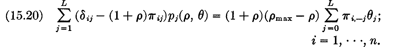
If we let v(ρ, 0) be the vector whose ith component is

and let p₁(ρ, θ) be the vector of length n whose components are P_j(ρ, θ), j = 1, . . ., n, we may write the solution of (15.20) in vectorial form as

This formula makes it evident that the proof of the present lemma will result immediately once we establish the following lemma.

LEMMA 15.8. Let A be a connected positive matrix with dom (A) < 1, and let a be determined by the equation dom ((1 + α) A) = 1, i.e., α = (dom (A))^–1 – 1. Then the matrix

is continuous and strictly positive in the whole closed interval 0 ≤ ρ ≤ α.

Proof: The correctness of our statement in the interval 0 ≤ ρ < a follows at once from Lemmas 3.3, 3.5, and 3.6. Thus we have only to show that the matrix (15.22) has a limit as ρ approaches α from below, and that this limiting matrix is positive.

Let v be the dominant eigenvector of A, so that (1 + a) Av = v. Then

so that J(ρ)v is bounded. Since every component of v is positive, and since all the entries of J(ρ) are positive for ρ < a, it follows at once that J(ρ) remains bounded as ρ → a. Thus we may extract a convergent subsequence from the family of matrices J(ρ); i.e., we may find a sequence ρ_n → α such that the sequence of matrices has a limit: lim_n→∞ J(ρ_n) = J. Since the limit of a sequence of nonnegative matrices is nonnegative, it follows from (15.23) that J is nonnegative and Jv = (1 + α)v.

Since (I – (1 + ρ)A)J(ρ) = (α – ρ), it follows on letting ρ approach α that (1 + α)AJ = J; thus every column of the matrix J must be proportional to the column vector v; similarly, we may show that every row of the matrix J must be proportional to the uniquely defined adjoint vector u´ which satisfies u(l + α)A = u’. Hence the elements J _ik of J must have the form J _ik = cv_iu_k. Since (1 + α)Jv = (1 + α)v, we must have cu’v = 1 + α, so that c = (u’v)^–1(l + α) is positive, and thus J is positive and uniquely defined.

Let ρ’_n be any other sequence of numbers approaching α from below for which lim_n→∞ J(ρ’n) = J’ exists. Then, by the argument of the preceding paragraph, we must have J’ = J. This shows that lim_ρ→∞ J(ρ) = J exists, establishing the continuity and positivity of J(ρ) in the closed interval 0 ≤ ρ ≤ α, and completing the proof of the present lemma and of Lemma 7. Q.E.D.

Next we give a lemma generalizing the key Lemma 2 of the preceding section.

LEMMA 15.9. Let ϕ_–j(ρ, θ) = –d_–j(ρ, θ) – s_–j(ρ, θ), j = 0, . . ., L as above, and put

where Moreover, put

and

Then

Moreover,

Proof: By (15.11), (15.13), (15.14), and (15.15) we have

Our lemma follows immediately on using the definitions (15.25) and (15.26). Q.E.D.

We may now conveniently make use of a result from elementary topology.

To state this result, we have first to make a number of simple geometric definitions.

DEFINITION. The k-dimensional simplex is the subset σ of Euclidean k + 1-dimensional space defined by the formula

DEFINITION. The vertices of the k-dimensional simplex σ are the k + 1 points p^(j) defined by

DEFINITION. Let p^(j1) , · · ·, p^(jr) be a set of r distinct vertices of the simplex σ. Then the side determined by these vertices is the subset σ₀ of a defined by the formula

In terms of these definitions we may state the following useful topological theorem.

THEOREM 15.10. Suppose an n – 1-dimensional simplex is covered by n closed sets in such a way that for each r the r – 1-dimensional side determined by the vertices p_i1,· · ·, p_ir is contained in the union of the m sets Then the sets have a common point, i.e.,

(For an elementary proof, see L. Graves, Theory of Functions of Real Variables (1946 Edn., p. 148).)

We can use this theorem to establish the following.

LEMMA 15.11. Let σ be the simplex defined by

Let f_j(x₁, · · ·, x_k), j = 1, · · ·, k be continuous functions defined on σ such that

Then there is a point x₁⁰, · · ·, x_n⁰ such that for every j

with equality wherever

Proof: For each j = 1, · · ·, k define the closed set by writing

We first show that the r – 1-dimensional side σ’ of σ with vertices is contained in the union of the sets After permuting the variables x, we may assume without loss of generality that i₁, · · ·, i_r = 1 · · · r. Our side is then the subset of (15.32) defined by the equations

so that

everywhere along the side σ’. Therefore for each x in σ’, at least one function f_j must be nonnegative. Thus the side σ’ is contained in

By Theorem 12, then, the intersection of all the sets is not void. Any point in the intersection is a point satisfying the conditions of the present lemma. Q.E.D.

We may use Lemma 9 and Theorem 10 to derive the following lemma, which practically contains the main Theorem 6 which we are in the course of proving.

LEMMA 15.12. There exists a point ρ, θ such that

At this point we have ϕ_–j(ρ, θ) = 0 if j ≠ L+1 and p_–j(ρ, θ) ≠ 0, while ϕ–L–1(ρ, θ) = 0 if ρ ≠ 0.

Proof: Let 0*_i, i = 0, · · ·, L + 1 be the quantities defined in the statement of Lemma 9. Since ρ may be varied arbitrarily between 0 and ρ_max, and since the quantities θ_j may be varied arbitrarily subject only to the restrictions θ_j ≥ 0 and it is plain that by choosing ρ and θ, the quantities θ*_j may be varied arbitrarily subject only to the restrictions (15.28). It is clear from (15.25) and (15.26) that as long as θ*_L+1 ≠ 1, i.e., as long as ρ ≠ ρ_max, we may write ρ and θ as continuous functions of θ*:

Thus the functions ϕ_–j(ρ(θ*), θ(θ*)) depend continuously on θ* except at the vertex θ*_L+1 = 1. However, since (cf. Lemma 15.7) p_–j(ρ, θ) = θ*_j even in the vicinity of ρ = ρ_max, it follows from (15.11), (15.12)–(15.14), (15.15), (15.16) and the formula following (15.16), and (15.24)–(15.26) that ϕ_–j(ρ(θ*), θ(θ*)) depends continuously on θ* even near θ*_L+1 = 1. Thus, by Lemma 11, there exists a ρ and θ such that ϕ_–j(ρ, θ) ≥ 0, j = 0, · · ·, L + 1, with equality if 0*_j ≠ 0.

Using (15.25) and (15.26), the present lemma follows at once. Q.E.D.

LEMMA 15.13. A point ρ = 0 satisfies

if and only if

Proof: Use the identity

given by Lemma 9; differentiate and put ρ = 0. Q.E.D.

Now we shall prove part A of Theorem 6.

Proof of Part A of Theorem 6. Suppose first that ρ > 0. Let ρ, θ be a rate of profit and a set of wage ratios such that ϕ_–j(ρ, θ) ≥ 0, 0 ≤ j ≤ L + 1 with equality whenever θ_j ≠ 0. It is clear from Lemma 10 that not all the prices p_j(ρ, θ) are zero; thus condition (a) is satisfied. Since the consumption schemes s_j^(v)(ρ, θ) are determined by (15.12)–(15.13), they satisfy condition (c). Since the total activity levels a_i(ρ, θ) are defined by (15.15) and since by hypothesis we have ϕ_–j(ρ, θ) ≥ 0 with equality whenever p_–j(ρ, θ) ≠ 0, we see that condition (d) is also satisfied. It only remains to show that condition (b) is satisfied; since with prices giving a uniform positive rate of profit a firm makes maximum profits if and only if it employs all its capital it is sufficient to show that the total activity levels a_i(ρ, θ) can be divided into the sum of individual-firm contributions a_i^(k) in such a way that

and

It is plain that (15.38) and (15.39) can be satisfied simultaneously if and only if

where Formula (15.24) shows that (15.40) holds, since, by hypothesis, ϕ_–j(ρ, θ) = 0 unless p_–j(ρ, θ) = 0.

Conversely, suppose that we have a price equilibrium corresponding to the rate of profit ρ > 0 and the wage ratios θ. We know that condition (b) implies that the equilibrium prices are (proportional to) p_j(ρ, θ), j = –L, · · ·, n. Since we have seen that all the prices p_j(ρ, θ), j = 1, · · ·, n are then strictly positive, it follows from condition (d) that the total activity levels must satisfy (15.15). Moreover, by condition (b), each firm must employ its total capital; thus, the dividend income of the vth family is necessarily given by

which by condition (c) implies that the family’s labor-consumption scheme must satisfy (15.12)–(15.13). Next we observe that condition (d) implies that at equilibrium we have ϕ_–j(ρ, θ) ≥ 0, with equality if p_–j(ρ, θ) ≠ 0. Thus part A of Theorem 6 is proved in case ρ > 0.

If ρ = 0, we may argue in almost the same way, making use however of the information given by Lemma 13. We have only to amend the sixth sentence of the first paragraph of the present proof to state that if ρ = 0, a firm makes no profit in any case, so that condition (e) degenerates by the further argument of the present proof to the condition

i.e., to the condition ϕ_–L–1(0, θ) ≥ 0. The converse argument in case ρ = 0 is again much like the converse argument in case ρ > 0; we have only to amend the preceding paragraph with the remark that if profits are all zero, dividend income for each family is zero also. Thus part A of Theorem 6 is fully proved.

Proof of Part B of Theorem 6: This follows at once from Part A and from Lemmas 12 and 13. Q.E.D.

4.A Summary Remark

The analysis presented in the present lecture shows the Walrasian theory to be quite satisfactory from the purely mathematical point of view. On the other hand, we have seen above that its mathematical formulations are based upon unrealistically drastic assumptions, which artificially assume away all the Keynesian phenomena studied in Lectures 5–12. In order to incorporate the neoclassical ideas of the three preceding lectures into a less hopelessly unrealistic model, it is necessary for us to construct a generalized equilibrium model combining neoclassical and Keynesian features. We now turn to this task.