Summary. Discrete random variables are studied via their probability mass functions. This leads to the definition of the ‘mean value’ or ‘expectation’ of a random variable. There are discussions of variance, and of functions of random variables. Methods are presented for calculating expectations, including the use of conditional expectation.

2.1 Probability mass functions

Given a probability space , we are often interested in situations involving some real-valued function X acting on Ω. For example, let be the experiment of throwing a fair die once, so that , and suppose that we gamble on the outcome of in such a way that the profit is

where negative profits are positive losses. If the outcome is ω, then our profit is , where is defined by

The mapping X is an example of a ‘discrete random variable’.

More formally, a discrete random variable X on the probability space is defined to be a mapping such that ¹

(2.1)

(2.2)

The word ‘discrete’ here refers to the condition that X takes only countably many values in .² Condition (2.2) is obscure at first sight, and the point here is as follows. A discrete random variable X takes values in , but we cannot predict the actual value of X with certainty since the underlying experiment involves chance. Instead, we would like to measure the probability that X takes a given value, x say. To this end, we note that X takes the value x if and only if the result of lies in that subset of Ω which is mapped into x, namely the subset . Condition (2.2) postulates that all such subsets are events, in that they belong to , and are therefore assigned probabilities by .

The most interesting things about a discrete random variable are the values which it may take and the probabilities associated with these values. If X is a discrete random variable on the probability space (), then its image is the image of Ω under X, that is, the set of values taken by X.

Henceforth, we abbreviate events of the form to the more convenient form .

Definition

The (probability) mass function (or pmf) of the discrete random variable X is the function defined by

(2.4)

Thus, is the probability that the mapping X takes the value x. Note that is countable for any discrete random variable X, and

(2.5)

(2.6)

Equation (2.6) is sometimes written as

in the light of the fact that only countably many values of x make non-zero contributions to this sum. Condition (2.6) essentially characterizes mass functions of discrete random variables in the sense of the following theorem.

Theorem 2.7

Let be a countable set of distinct real numbers, and let be a collection of real numbers satisfying

There exists a probability space and a discrete random variable X on such that the probability mass function of X is given by

Proof

Take , to be the set of all subsets of Ω, and

Finally, define by for .

This theorem is very useful, since for many purposes it allows us to forget about sample spaces, event spaces, and probability measures; we need only say ‘let X be a random variable taking the value s_i with probability , for ’ and we can be sure that such a random variable exists without having to construct it explicitly.

In the next section, we present a list of some of the most common types of discrete random variables.

Exercise 2.8

If X and Y are discrete random variables on the probability space (), show that U and V are discrete random variables on this space also, where

Exercise 2.9

Show that if is the power set of Ω, then all functions which map Ω into a countable subset of are discrete random variables.

Exercise 2.10

If E is an event of the probability space show that the indicator function of E, defined to be the function on Ω given by

is a discrete random variable.

Exercise 2.11

Let () be a probability space in which

and let U, V, W be functions on Ω defined by

for . Determine which of U, V, W are discrete random variables on the probability space.

Exercise 2.12

For what value of c is the function p, defined by

a mass function?

2.2 Examples

Certain types of discrete random variables occur frequently, and we list some of these. Throughout this section, n is a positive integer, p is a number in , and . We never describe the underlying probability space.

Bernoulli distribution. This is the simplest non-trivial distribution. We say that the discrete random variable X has the Bernoulli distribution with parameter p if the image of X is , so that X takes the values 0 and 1 only.

Such a random variable X is often called simply a coin toss. There exists such that

(2.13)

and the mass function of X is given by

Coin tosses are the building blocks of probability theory. There is a sense in which the entire theory can be constructed from an infinite sequence of coin tosses.

Binomial distribution. We say that X has the binomial distribution with parameters n and p if X takes values in and

(2.14)

Note that (2.14) gives rise to a mass function satisfying (2.6) since, by the binomial theorem,

Poisson distribution. We say that X has the Poisson distribution with parameter λ () if X takes values in and

(2.15)

Again, this gives rise to a mass function since

Geometric distribution. We say that X has the geometric distribution with parameter if X takes values in and

(2.16)

As before, note that

Negative binomial distribution. We say that X has the negative binomial distribution with parameters n and if X takes values in and

(2.17)

As before, note that

using the binomial expansion of , see Theorem A.3.

Example 2.18

Here is an example of some of the above distributions in action. Suppose that a coin is tossed n times and there is probability p that heads appears on each toss. Representing heads by H and tails by T, the sample space is the set Ω of all ordered sequences of length n containing the letters H and T, where the kth entry of such a sequence represents the result of the kth toss. The set Ω is finite, and we take to be the set of all subsets of Ω. For each , we define the probability that ω is the actual outcome by

where is the number of heads in ω and is the number of tails. Similarly, for any ,

For we define the discrete random variable X_i by

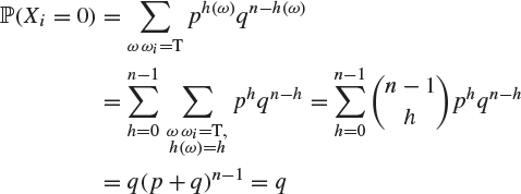
Each X_i takes values in and has mass function given by

where is the ith entry in ω. Thus

and

Hence, each X_i has the Bernoulli distribution with parameter p. We have derived this fact in a cumbersome manner, but we believe these details to be instructive.

Let

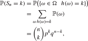
which is to say that . Clearly, S_n is the total number of heads which occur, and S_n takes values in since each X_i equals 0 or 1. Also, for we have that

(2.19)

and so S_n has the binomial distribution with parameters n and p.

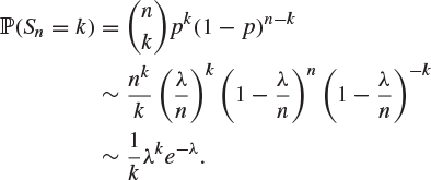
If n is very large and p is very small but np is a ‘reasonable size’ (, say) then the distribution of S_n may be approximated by the Poisson distribution with parameter λ, as follows. For fixed , write and suppose that n is large to find that

(2.20)

This approximation may be useful in practice. For example, consider a single page of the Guardian newspaper containing, say, characters, and suppose that the typesetter flips a coin before setting each character and then deliberately mis-sets this character whenever the coin comes up heads. If the coin comes up heads with probability on each flip, then this is the equivalent to taking and in the above example, giving that the number S_n of deliberate mistakes has the binomial distribution with parameters and . It may be easier (and not too inaccurate) to use (2.20) rather than (2.19) to calculate probabilities. In this case, and so, for example,

Example 2.21

Suppose that we toss the coin of the previous example until the first head turns up, and then we stop. The sample space now is

where represents the outcome of k tails followed by a head, and represents an infinite sequence of tails with no head. As before, is the set of all subsets of Ω, and is given by the observation that

Let Y be the total number of tosses in this experiment, so that for and . If , then

showing that Y has the geometric distribution with parameter p.

Example 2.22

If we carry on tossing the coin in the previous example until the nth head has turned up, then a similar argument shows that, if , the total number of tosses required has the negative binomial distribution with parameters n and p.

Exercise 2.23

If X is a discrete random variable having the Poisson distribution with parameter λ, show that the probability that X is even is .

Exercise 2.24

If X is a discrete random variable having the geometric distribution with parameter p, show that the probability that X is greater than k is .

2.3 Functions of discrete random variables

Let X be a discrete random variable on the probability space and let . It is easy to check that is a discrete random variable on also, defined by

Simple examples are

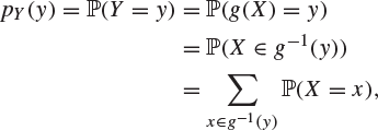
If , the mass function of Y is given by

(2.25)

since there are only countably many non-zero contributions to this sum. Thus, if with , then

while if , then

Exercise 2.26

Let X be a discrete random variable having the Poisson distribution with parameter λ, and let . Find the mass function of Y.

2.4 Expectation

Consider a fair die. If it were thrown a large number of times, each of the possible outcomes would appear on about one-sixth of the throws, and the average of the numbers observed would be approximately

which we call the mean value. This notion of mean value is easily extended to more general distributions as follows.

Definition 2.27

If X is a discrete random variable, the expectation of X is denoted by and defined by

(2.28)

whenever this sum converges absolutely, in that .

Equation (2.28) is often written

and the expectation of X is often called the expected value or mean of X.³ The reason for requiring absolute convergence in (2.28) is that the image may be an infinite set, and we need the summation in (2.28) to take the same value irrespective of the order in which we add up its terms.

The physical analogy of ‘expectation’ is the idea of ‘centre of gravity’. If masses with weights are placed at the points of , then the position of the centre of gravity is , or , where is the proportion of the total weight allocated to position x_i.

If X is a discrete random variable (on some probability space) and , then is a discrete random variable also. According to the above definition, we need to know the mass function of Y before we can calculate its expectation. The following theorem provides a useful way of avoiding this tedious calculation.

Theorem 2.29 (Law of the subconscious statistician)

If X is a discrete random variable and , then

whenever this sum converges absolutely.

Intuitively, this result is rather clear, since takes the value when X takes the value x, an event which has probability . A more formal proof proceeds as follows.

Proof

Writing I for the image of X, we have that has image . Thus

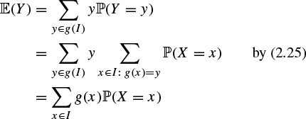
if the last sum converges absolutely.

Two simple but useful properties of expectation are as follows.

Theorem 2.30

Let X be a discrete random variable and let .

(a) If and , then .

(b) We have that .

Proof

(a) Suppose the assumptions hold. By the definition (2.28) of , we have that for all . Therefore, for , and the claim follows.

(b) This is a simple consequence of Theorem 2.29 with .

Here is an example of Theorem 2.29 in action.

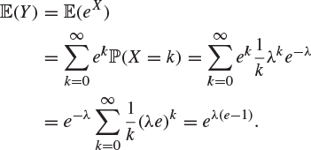
Example 2.31

Suppose that X is a random variable with the Poisson distribution, parameter λ, and we wish to find the expected value of . Without Theorem 2.29 we would have to find the mass function of Y. Actually this is not difficult, but it is even easier to apply the theorem to find that

The expectation of a discrete random variable X is an indication of the ‘centre’ of the distribution of X. Another important quantity associated with X is the ‘variance’ of X, and this is a measure of the degree of dispersion of X about its expectation .

Definition 2.32

The variance of a discrete random variable X is defined by

(2.33)

We note that, by Theorem 2.29,

(2.34)

where . A rough motivation for this definition is as follows. If the dispersion of X about its expectation is very small, then tends to be small, giving that is small also; on the other hand, if there is often a considerable difference between X and its mean, then may be large, giving that is large also.

Equation (2.34) is not always the most convenient way to calculate the variance of a discrete random variable. We may expand the term in (2.34) to obtain

where as before. Thus we obtain the useful formula

(2.35)

Example 2.36

If X has the geometric distribution with parameter p (), the mean of X is

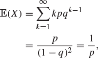
and the variance of X is

by (2.35).⁴ Now,

by Footnote 4, giving that

Exercise 2.37

If X has the binomial distribution with parameters n and , show that

and deduce the variance of X.

Exercise 2.38

Show that for .

Exercise 2.39

Find and when X has the Poisson distribution with parameter λ, and hence show that the Poisson distribution has variance equal to its mean.

2.5 Conditional expectation and the partition theorem

Suppose that X is a discrete random variable on the probability space , and that B is an event with . If we are given that B occurs, then this information affects the probability distribution of X. That is, probabilities such as are replaced by conditional probabilities such as .

Definition 2.40

If X is a discrete random variable and , the conditional expectation of X given B is denoted by and defined by

(2.41)

whenever this sum converges absolutely.

Just as the partition theorem, Theorem 1.48, expressed probabilities in terms of conditional probabilities, so expectations may be expressed in terms of conditional expectations.

Theorem 2.42 (Partition theorem)

If X is a discrete random variable and is a partition of the sample space such that for each i, then

(2.43)

whenever this sum converges absolutely.

Proof

The right-hand side of (2.43) equals, by (2.41),

We close this chapter with an example of this partition theorem in use.

Example 2.44

A coin is tossed repeatedly, and heads appears at each toss with probability p, where . Find the expected length of the initial run (this is a run of heads if the first toss gives heads, and of tails otherwise).

Solution

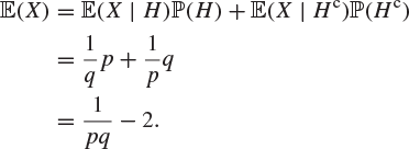
Let H be the event that the first toss gives heads and the event that the first toss gives tails. The pair H, forms a partition of the sample space. Let X be the length of the initial run. It is easy to see that

since if H occurs, then if and only if the first toss is followed by exactly heads and then a tail. Similarly,

Therefore,

and similarly,

By the partition theorem, Theorem 2.42,

Exercise 2.45

Let X be a discrete random variable and let g be a function from to . If x is a real number such that , show formally that

and deduce from the partition theorem, Theorem 2.42, that

Exercise 2.46

Let N be the number of tosses of a fair coin up to and including the appearance of the first head. By conditioning on the result of the first toss, show that .

2.6 Problems

1. If X has the Poisson distribution with parameter λ, show that

for .

2. Each toss of a coin results in heads with probability p (). If is the mean number of tosses up to and including the rth head, show that

for , with the convention that . Solve this difference equation by the method described in Appendix B.

3. If X is a discrete random variable and , show that . Deduce that, if , then , whenever is finite.

4. For what values of c and α is the function p, defined by

a mass function?

5. Lack-of-memory property. If X has the geometric distribution with parameter p, show that

for m, .

We say that X has the ‘lack-of-memory property’ since, if we are given that , then the distribution of is the same as the original distribution of X. Show that the geometric distribution is the only distribution concentrated on the positive integers with the lack-of-memory property.

6. The random variable N takes non-negative integer values. Show that

provided that the series on the right-hand side converges.

A fair die having two faces coloured blue, two red and two green, is thrown repeatedly. Find the probability that not all colours occur in the first k throws.

Deduce that, if N is the random variable which takes the value n if all three colours occur in the first n throws but only two of the colours in the first throws, then the expected value of N is . (Oxford 1979M)

7. Coupon-collecting problem. There are c different types of coupon, and each coupon obtained is equally likely to be any one of the c types. Find the probability that the first n coupons which you collect do not form a complete set, and deduce an expression for the mean number of coupons you will need to collect before you have a complete set.

*8. An ambidextrous student has a left and a right pocket, each initially containing n humbugs. Each time he feels hungry, he puts a hand into one of his pockets and, if it is not empty, he takes a humbug from it and eats it. On each occasion, he is equally likely to choose either the left or right pocket. When he first puts his hand into an empty pocket, the other pocket contains H humbugs.

Show that if p_h is the probability that , then

and find the expected value of H, by considering

or otherwise. (Oxford 1982M)

9. The probability of obtaining a head when a certain coin is tossed is p. The coin is tossed repeatedly until n heads occur in a row. Let X be the total number of tosses required for this to happen. Find the expected value of X.

10. A population of N animals has had a certain number a of its members captured, marked, and then released. Show that the probability P_n that it is necessary to capture n animals in order to obtain m which have been marked is

where . Hence, show that

and that the expectation of n is . (Oxford 1972M)